First-Order Individual Gas Sensors as Next Generation Reliable Analytical Instruments

Abstract

It is conventionally expected that the performance of existing gas sensors may degrade in the field compared to laboratory conditions because (i) a sensor may lose its accuracy in the presence of chemical interferences and (ii) variations of ambient conditions over time may induce sensor-response fluctuations (i.e., drift). Breaking this status quo in poor sensor performance requires understanding the origins of design principles of existing sensors and bringing new principles to sensor designs. Existing gas sensors are single-output (e.g., resistance, electrical current, light intensity, etc.) sensors, also known as zero-order sensors (Karl Booksh and Bruce R. Kowalski, Analytical Chemistry, DOI: 10.1021/ac00087a718). Any zero-order sensor is undesirably affected by variable chemical background and sensor drift that cannot be distinguished from the response to an analyte. To address these limitations, we are developing multivariable gas sensors with independent responses, which are first-order analytical instruments. Here, we demonstrate self-correction against drift in two types of first-order gas sensors that operate in different portions of the electromagnetic spectrum. Our radiofrequency sensors utilize dielectric excitation of semiconducting metal oxide materials on the shoulder of their dielectric relaxation peak and achieve self-correction of the baseline drift by operation at several frequencies. Our photonic sensors utilize nanostructured sensing materials inspired by Morpho butterflies and achieve self-correction of the baseline drift by operation at several wavelengths. These principles of self-correction for drift effects in first-order sensors open opportunities for diverse emerging monitoring applications that cannot afford frequent periodic maintenance that is typical of traditional analytical instruments.

Graphical Abstract

This is a visual representation of the abstract.

Keywords

Zero-order sensor first-order sensor multivariable gas sensor dielectric excitation semiconducting metal oxide photonic nanostructure self-correction for sensor drift

Introduction

Recent advances in classic single-output gas sensors include high sensitivity down to a few molecules in clean air and subsecond response times.^1,2 However, once the number of background chemicals increases, existing sensors lose their accuracy because of two key reasons. First, gas-sensing material interactions that provide a reversible sensor response to an analyte gas also allow a response to interfering volatiles.³ Second, design principles of existing sensors to have only one output are adequate for detection of relatively high levels of gases, for example, for safety against toxic and flammable gases.^4,5 In the detection of trace gas levels, “the biggest headaches are caused by interfering chemicals", stated in a Nature paper.⁶ Effects of interferences make the data from sensors “essentially meaningless,” stated in another Nature paper.⁷ An additional deficiency of single-output sensors is their accuracy loss over time because of drift.^8,9 Arranging sensors into arrays makes the system drift worse since each sensor independently contributes to system drift.¹⁰ Forty years after the first sensor arrays,^11–13 drift remains a persistent problem.^14,15 Thus, innovations are needed in gas sensor designs in two directions to prevail over the limitations of existing sensors: (i) to improve sensor selectivity for accurate detection of one or more analyte gases in complex chemical backgrounds and (ii) to improve sensor stability.

To expand opportunities for gas sensors, the mathematics behind their design principles should be revised. Gas sensors originate from the 1930s to the 1970s^4,5 as single-output (e.g., resistance, electrical current, light intensity, etc.) sensors, also known as zero-order sensors.¹⁶ They are affected by variable chemical backgrounds and sensor drift that cannot be distinguished from an analyte response, indicated by academic studies,^6,7 regulatory agencies,^17,18 and end-users.¹⁹ To overcome the limitations of existing sensors, new gas sensors should be designed as the first- and higher-order devices.

Previously, we introduced multivariable gas sensors with multiple outputs as the first-order sensors to address the problems of zero-order sensors.^10,20–37 These sensors demonstrated four-dimensional sensor dispersion,^10,37 differentiated complex odors,³⁷ vapors of the same dielectric constant,^24,37 closely related volatiles such as straight-chain C1–C9 primary alcohols^10,37 and C1–C3 hydrocarbons,²⁷ quantified gases mixed with uncalibrated interferences,²⁶ rejected interferences up to 2 × 10⁶-fold,^27,37 and quantified analytes in quaternary mixtures.^27,30,32,37

In this study, we introduce methodologies to improve the stability of two types of our multivariable (first-order) sensors. Radiofrequency (RF) sensors perform dielectric excitation of semiconducting metal oxide (SMOX) materials on the shoulder of their dielectric relaxation peak and reject baseline drift through operation at several frequencies. Photonic sensors utilize nanostructured sensing materials and reject baseline drift through operation at several wavelengths. Multivariate curve resolution (MCR) algorithms of the first-order data¹⁶ from multivariable sensors are also explored with the inspiration of achieving a second-order advantage.^38,39

Toward High Stability of First-Order Gas Sensors

To differentiate volatiles in complex backgrounds, instrument designs with one or more independent measurement variables (outputs) are utilized.¹⁶ High-performance capabilities of traditional analytical instruments are provided by independent variables in their outputs making these instruments first- and higher-order devices. Examples of independent variables include retention time in gas chromatography, the mass-to-charge ratio in mass spectrometry, drift time in ion mobility, or wavelengths in infrared spectroscopic systems. These and other independent variables facilitate selective detection of analytes and rejection of interferences. The value of independent response variables in analytical instruments has been recognized with the Nobel Prizes for partition chromatography, laser spectroscopy, and mass spectrometry.⁴⁰

Multivariable (first-order) gas sensors are built following the mathematics of traditional analytical instruments but provide different types of independent variables for multigas detection. There are four design criteria for first-order gas sensors. First, a sensing material is utilized with diverse responses to different gases. Second, a multivariable transduction methodology is applied to provide independent outputs to recognize these different gas responses and to support the self-correction of drift. Third, the excitation conditions of the first-order sensor are determined to maximize different gas responses and to facilitate self-correction of drift. Fourth, data analytics is employed to provide multianalyte quantitation, rejection of interferences, and drift minimization.

Traditional analytical instruments rely on their periodic maintenance to yield their exquisite performance. Table I shows timelines of maintenance requirements of analytical instruments approved for monitoring the key pollutants in outdoor ambient air and for homeland security uses. These requirements range from “a provided calibration standard should be used prior to each use", to a “minimum of one multipoint calibration per quarter", and to “multipoint calibration every 12 months".^41–46 However, it is expected that, unlike traditional analytical instruments, gas sensors should be able to produce accurate results without periodic expert maintenance.

Table I.

Timelines of maintenance requirements of illustrative traditional analytical instruments approved for monitoring of the key pollutants in outdoor ambient air (O₃, CO, SO₂, and NO₂) and homeland security applications.^41–46

Detection principle		Calibration frequency
UV photometry	O₃ Analyzer 2B Technologies Model 211	Zeroing (preferably daily) using an external ozone scrubber Multipoint calibration every 12 months or within a mandated calibration frequency
Nondispersive infrared photometry	CO Analyzer Yokogawa Model IR400	Zero calibration and span calibration once a week using a standard gas cylinder
Pulsed UV fluorescence	SO Analyzer Thermo Sdentific™ Model 43i	Normally, zero and span are checked daily As experience is gained with an instrument, the frequency of these checks can be adjusted
Chemiluminescence	NO–NO₂–NO_x Analyzer Thermo Scientific™ Model 42i	Minimum of one multipoint calibration per calendar quarter Stability of the zero and span checks run daily
GC-MS	Inficon AG HAPSITE ER	To continue running samples after 12 h, use the 50 ppb calibration standard as the CCC Internal standard canister to be replaced after 3 days of continuous use
IMS	Smiths Detection JCAD LCD 3 3 Lightweight Chemical Detector	Provided calibration standard should be used prior to each use

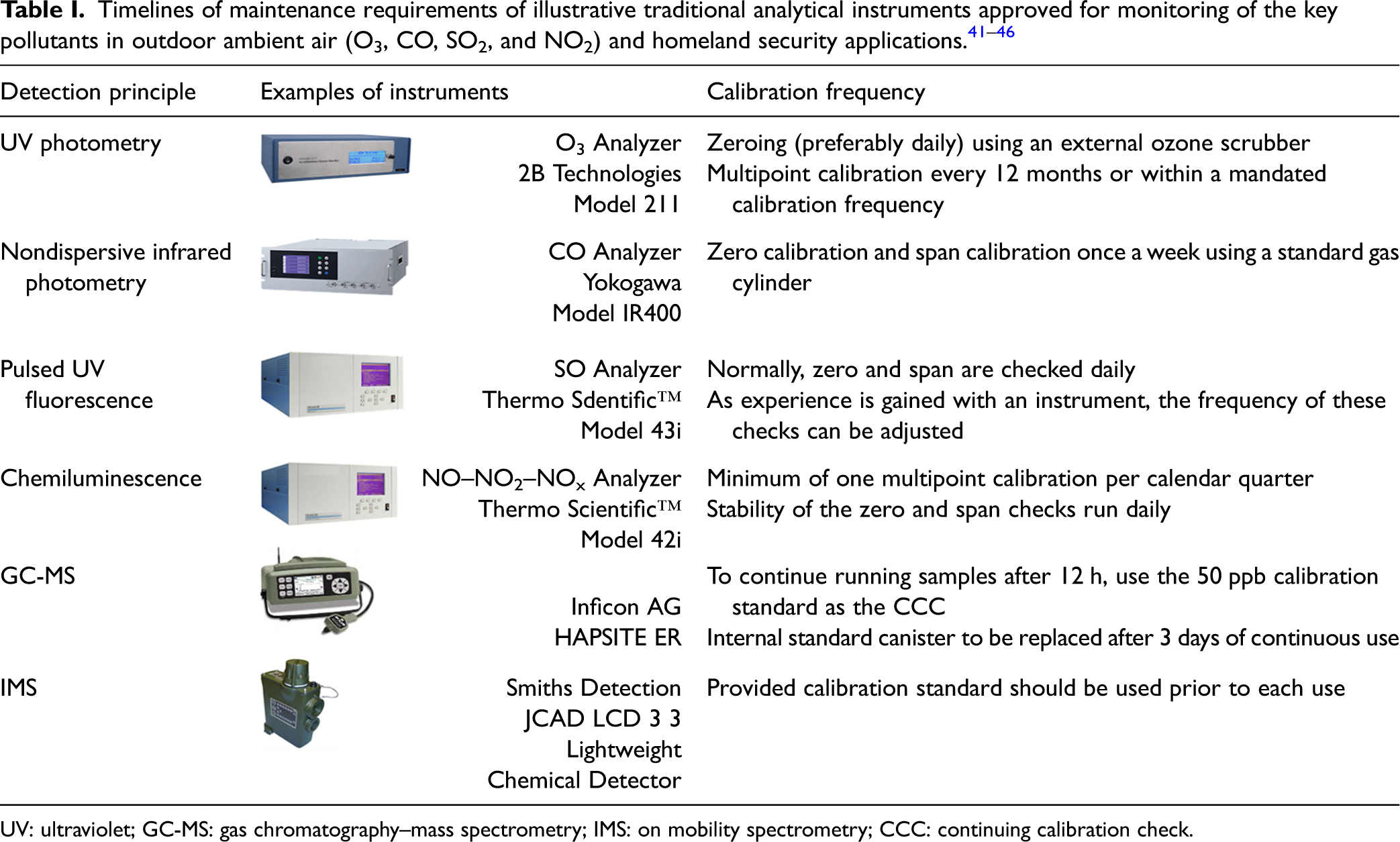
UV: ultraviolet; GC-MS: gas chromatography–mass spectrometry; IMS: on mobility spectrometry; CCC: continuing calibration check.

Figure 1 summarizes the effects of drift in zero-order (single-output) gas sensors, traditional analytical instruments, and first-order (multivariable) gas sensors. When a gas response of a zero-order sensor is comparable to the level of drift (Fig. 1a), the effects of drift will lead to false alarms. Traditional analytical instruments periodically are recalibrated to avoid this problem (Fig. 1b). The first-order (multivariable) gas sensors have the ability to self-correct from the effects of drift (Fig. 1c). This self-correction is achieved by operation at more than one frequency or wavelength across the operating range of our multivariable gas sensors.

Figure 1.

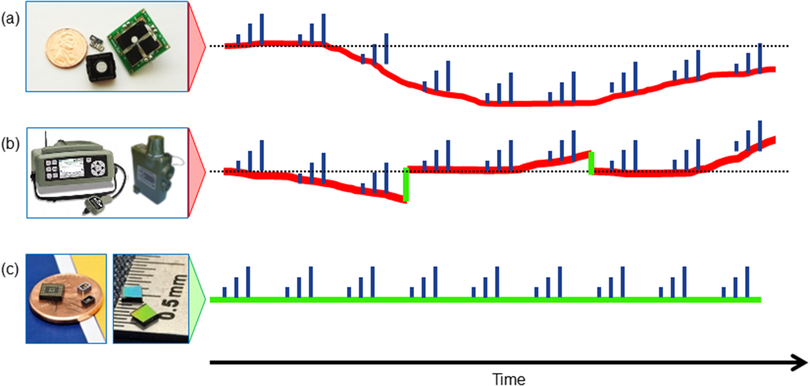
Effects of baseline drift in three categories of analytical instruments. (a) Undetected accuracy loss of a single-output gas sensor. When the sensor response to a small concentration of a gas is comparable with the level of baseline drift, the sensor effects by the drift can cause false alarms. (b) Periodical resets and/or recalibrations of traditional analytical instruments to achieve desired measurement accuracy. (c) Concept of operation of our multivariable sensors with a self-correction for effects of baseline drift. This highly desired self-correction is achieved by operating at more than one frequency across the operating frequency range of our sensors.

Experimental

Exposures to Volatiles

Different concentrations of volatiles and their mixtures were produced using custom-built computer-controlled gas generation and mixing systems with complementary capabilities as detailed previously.^{27,28,31–34}

Sensing Elements

SMOX sensing elements were fabricated by state-of-the-art manufacturing practices as detailed previously.²⁷ Polymeric photonic nanostructures were fabricated, as detailed previously.³²

Sensor Data Acquisition

Impedance spectra of SMOX sensors were measured using laboratory and application-specific integrated circuit (ASIC) impedance analyzers as detailed previously.²⁷ Measurements of photonic nanostructures were performed using a broadband white light source in the reflectance mode as detailed previously.³²

Analysis of Sensor Data

Analysis of sensor data was done using KaleidaGraph (Synergy Software), Python (Python Software Foundation), and Matlab (The Mathworks Inc.). Multivariate data processing was done in Matlab and Python.

Receiver Operating Characteristic (ROC) Curves

The ROC curves illustrate the diagnostic ability of a binary classifier system, as its discrimination threshold is varied.⁴⁷ ROC curves were built in Python using all tested concentrations by plotting the true positive rate (probability of detection) against the false positive rate (probability of false alarms) at various threshold settings.⁴⁸

Multivariate Curve Resolution

Multivariate curve resolution (MCR) algorithms were implemented in Matlab. They explore mixtures of dynamic processes by deconstructing data sets with limited or absent reference information and system knowledge.⁴⁹ These approaches are also known as self-modeling mixture analysis, blind source separation, and spectral unmixing.⁵⁰

Results and Discussion

First-Order RF SMOX Gas Sensors

Principle of the First-Order RF SMOX Gas Sensors

In the first-order RF gas sensors, new attractive performance attributes of popular SMOX materials are provided by utilizing their new sensor-excitation scheme of impedance measurements of SMOX materials on the shoulder of their dielectric relaxation peak.²⁷

Figure 2 summarizes the conventional resistance readout and the multiband dielectric excitation on the shoulder of the dielectric relaxation peak of the SMOX sensing materials. Three highlighted frequency regions in Fig. 2 illustrate the high-frequency shoulder of the relaxation peak of an n-type SMOX material when exposed to various concentrations of a reducing gas. The dielectric excitation scheme of the SMOX gas-sensing materials unexpectedly provided the desired ability for multifrequency drift correction as discussed in the Multifrequency Self-Correction of Baseline Drift in the First-Order RF SMOX Gas Sensors section below.

Figure 2.

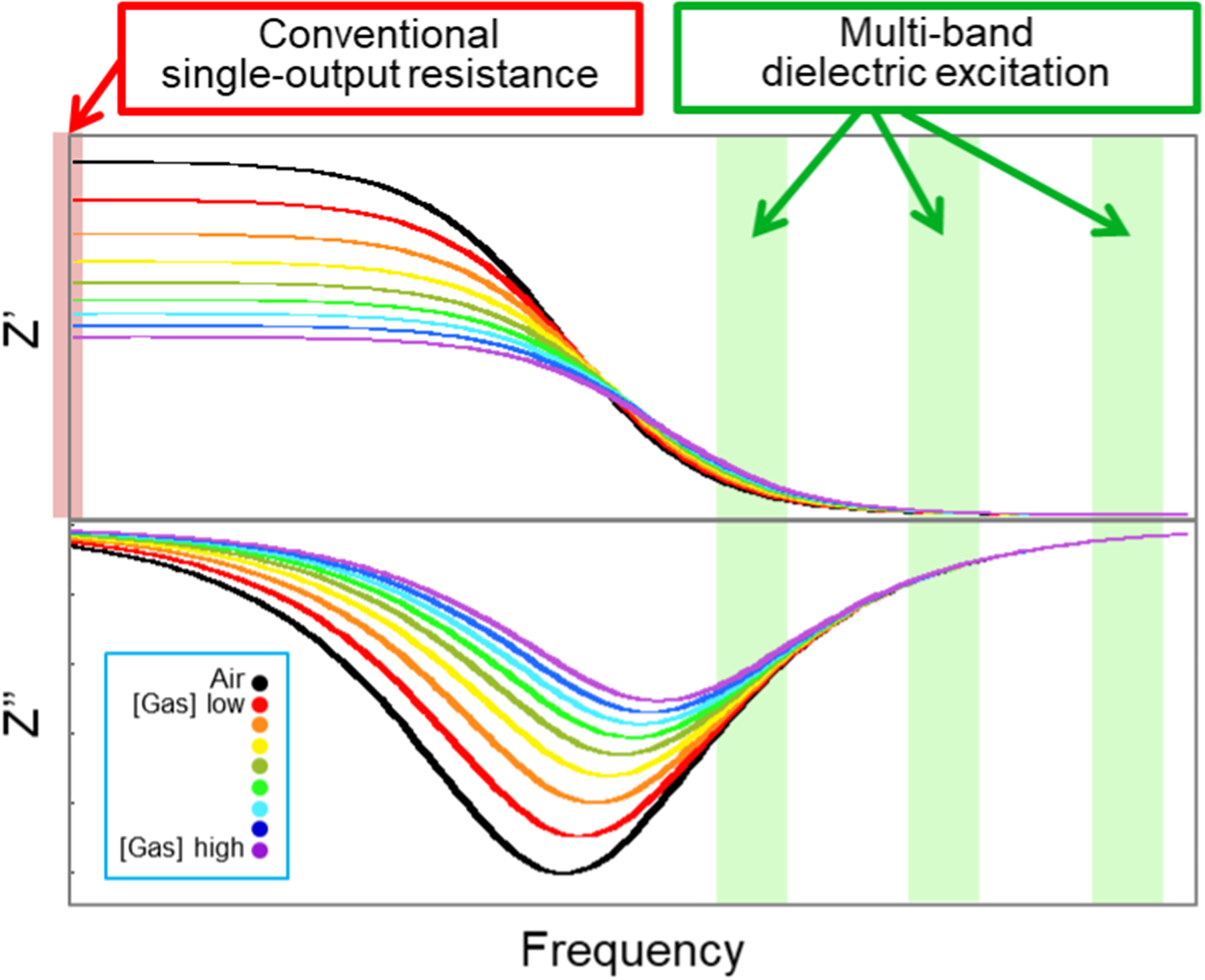
Gas-response readouts of SMOX sensing materials such as conventional single-output resistance and our multiband dielectric excitation on the shoulder of the dielectric relaxation peak of the material. Shown is an example of a sensor based on an n-type SMOX sensing material to a reducing gas.

Multifrequency Self-Correction of Baseline Drift in the First-Order RF SMOX Gas Sensors

While SMOX gas sensors under their dielectric excitation have stable responses (cf. Fig. S1, Supplemental Material), such stability can be affected by different environmental conditions leading to sensor drift. Baseline drift is an unsolved persistent problem in SMOX gas sensors with resistance readout.^8,9,15

To overcome this problem, two baseline correction algorithms are reported here. The first baseline correction algorithm works by operating the sensor at two frequencies, i.e., a low frequency with analytical information and drift, and a higher frequency with sensitivity to only drift. The two-frequency correction is based on our observation that there is a frequency region where the sensor contains baseline drift but with minimal or no signal at high frequencies. The second baseline correction algorithm works by operating the sensor at all operation frequencies.

An example of drift correction is shown in Fig. 3 for a SMOX sensing element exposed to NO₂ gas (an illustrative environmental pollutant) for more than 75 h in ambient lab conditions with 87 replicates of responses to 20, 40, 60, and 80 parts per billion (ppb) steps of NO₂ gas in the air. Three replicates of responses to four steps of NO₂ gas concentrations are depicted in Fig. 3a. For drift correction, the SMOX sensing element was operated at different frequencies (blue and green response traces for low and high frequencies, respectively (Fig. 3b). The combination of sensor operation at two frequencies has allowed for the correction of sensor drift (Fig. 3c). In zero-order sensors, baseline drift mathematically cannot be distinguished from the gas response.^51,52

Figure 3.

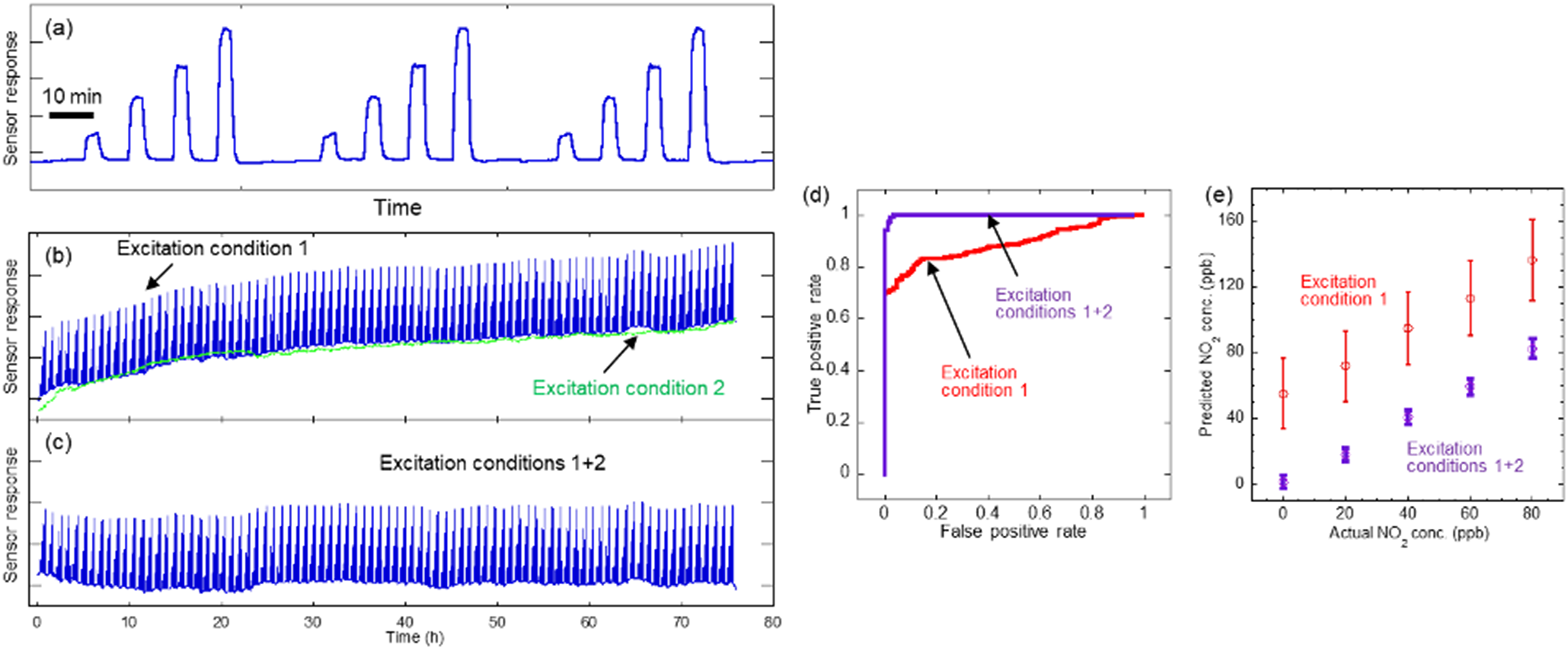
Two-frequency self-correction of baseline drift of a SMOX sensing element under its dielectric excitation during 87 replicate cycles of NO₂ exposures over more than 75 h of experiment. (a) Replicate (n = 3) responses of the sensor to NO₂ of 20, 40, 60, and 80 ppb. (b) Responses of the sensor to NO₂ for more than 75 h of experiment in ambient lab conditions with the depiction of relatively low and relatively high operational frequencies (excitation conditions 1 and 2, respectively). (c) Baseline-corrected response of the sensor. (d) ROC curves of the sensor for detection of NO₂ using excitation condition 1 (red line) and fusion of excitation conditions 1 + 2 (purple line) to reduce missed and false alarms. (e) Plots of actual concentrations versus predicted values of NO₂ concentrations before (red symbols) and after (purple symbols) drift correction.

One statistical metric of benefits of the self-correction of baseline drift is to analyze sensor response utilizing a ROC curve methodology.^47,48 Figure 3d shows ROC curves for the detection of NO₂ over the 87 replicates of exposures. One ROC curve was calculated using data only from one frequency (excitation condition 1). Another ROC curve was calculated when measurements were corrected by using the second excitation condition (excitation conditions 1 + 2). To achieve a true positive rate of 1.0, the false positive rate was 0.95 prior to drift correction and has improved by approximately thirtyfold to 0.03 after drift correction. Thus, sensor responses at selected frequencies maximized the true positive rate and minimized the false positive rate.

Another statistical metric of benefits of the self-correction of baseline drift is to analyze plots of actual concentrations versus predicted values before and after drift correction for their accuracy and precision of predicted gas concentrations.⁵³ Figure 3e shows plots over 87 replicates of exposures to NO₂ in the presence of drift (excitation condition 1) and when the drift was corrected by the combination of sensor operation at two frequencies (excitation conditions 1 + 2). The errors of predicted gas concentrations were from 52 to 56 ppb and from −2.0 to 2.5 ppb for the uncorrected and baseline-corrected sensor responses, respectively. The precision of the predicted NO₂ concentrations as 1 standard deviation (SD) from the mean was 21–25 ppb and 4.0–5.7 ppb for the uncorrected and corrected sensor responses, respectively.

In another example, the drift-correction methodology was implemented when detecting chemical warfare agent simulants such as dichloromethane (DCM) and 1,3-dichloropropane (DCP) at 0.39, 0.77, and 1.15 parts per million (ppm) in the air. Figure 4a illustrates three replicates of responses to these vapors. Figure 4b depicts the sensor response over 24 replicates of exposures to DCM and DCP for 25 h in ambient lab conditions. Response at an excitation condition 1 (blue response trace) shows the response to DCM and DCP and the sensor drift, while response at an excitation condition 2 (green response trace) shows only sensor drift. Operation at different frequencies allowed the correction of sensor drift as depicted in Fig. 4c. The response magnitude to DCM was comparable to the level of drift (see baseline response at 9 and 20 h of the experiment). The response magnitude to DCP was threefold larger than the amount of drift.

Figure 4.

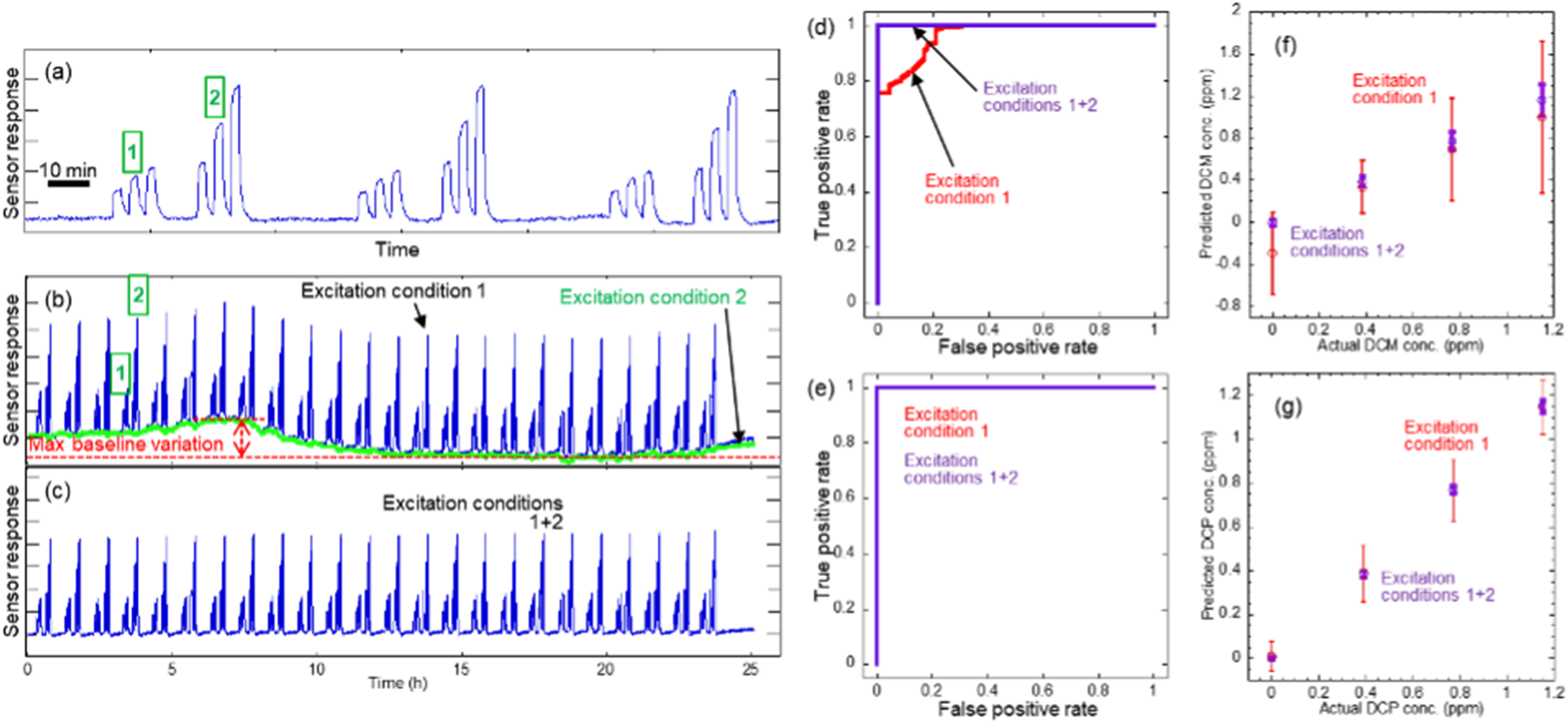
Two-frequency self-correction of baseline drift of a SMOX sensing element under its dielectric excitation during 24 replicate cycles of exposures to DCM (1) and DCP (2) vapors over 25 h of experiment. (a) Three replicates of sensor response to DCM and DCP, both vapors at concentrations of 0.39, 0.77, and 1.15 ppm. (b) Sensor response to DCM and DCP for 25 h of experiment in ambient lab conditions with a depiction of relatively low and relatively high operational frequencies (excitation conditions 1 and 2, respectively). (c) Baseline-corrected sensor response. ROC curves for detection of DCM (d) and DCP (e) using excitation condition 1 (red lines) and fusion of excitation conditions 1 + 2 (purple lines) to reduce missed and false alarms. For DCP, the signal-to-noise ratio was large enough that even without drift correction the true positive rate was 1.0 with a false positive rate of 0, thus red and purple lines completely overlapped. Plots of actual concentrations versus predicted values of DCM (f) and DCP (g) concentrations before (red symbols) and after (purple symbols) drift correction.

The ROC curves for detection of DCM and DCP over 24 replicates of exposures to DCM and DCP are presented in Figs. 4d and 4e when built using data only from one frequency (excitation condition 1) and from two frequencies for self-correction of baseline drift (excitation conditions 1 + 2). In DCM detection, to achieve a true positive rate of 1.0, the false positive rate was 0.31 prior to drift correction and improved to 0 after drift correction (Fig. 4d). For DCP, the signal-to-noise ratio was large enough that even without drift correction the true positive rate was 1.0 with a false positive rate of 0 (Fig. 4e).

Plots of actual versus predicted DCM concentrations before and after drift correction over 24 replicates of exposures to DCM are shown in Fig. 4f. The errors of predicted DCM concentrations were from −20 to −490 ppb and −1 to 9 ppb for the uncorrected and corrected sensor responses, respectively. The precision (as 1 SD from the mean) of the predicted DCM concentrations was 252–721 ppb and 31–149 ppb for the uncorrected and corrected sensor responses, respectively.

Similarly, plots of actual versus predicted DCP concentrations before and after drift correction are shown in Fig. 4g. The errors of predicted DCP concentrations were from −2 to 10 ppb and −7 to 0.1 ppb for the uncorrected and corrected sensor responses, respectively. The precision (as 1 SD from the mean) of the predicted DCM concentrations was 67–139 ppb and 6–27 ppb for the uncorrected and corrected sensor responses, respectively. Thus, because the sensor response to DCP was stronger as compared to DCM, the undesired effects of drift on the accuracy and precision of the sensor were less pronounced.

In the final example, an MCR analysis was performed on the measured sensor response using all operation frequencies of the ASIC impedance analyzer from 10 to 200 kHz. Figure 6 illustrates the responses of a SMOX sensing element to NO₂ gas to periodic exposures to 80, 160, and 240 ppb of NO₂ in the air over 45 h of the experiment in ambient lab conditions. While the baseline of the raw sensor response was fluctuating (Fig. 5a), the implementation of the MCR tool corrected the baseline drift as shown in Fig. 5b.

Figure 5.

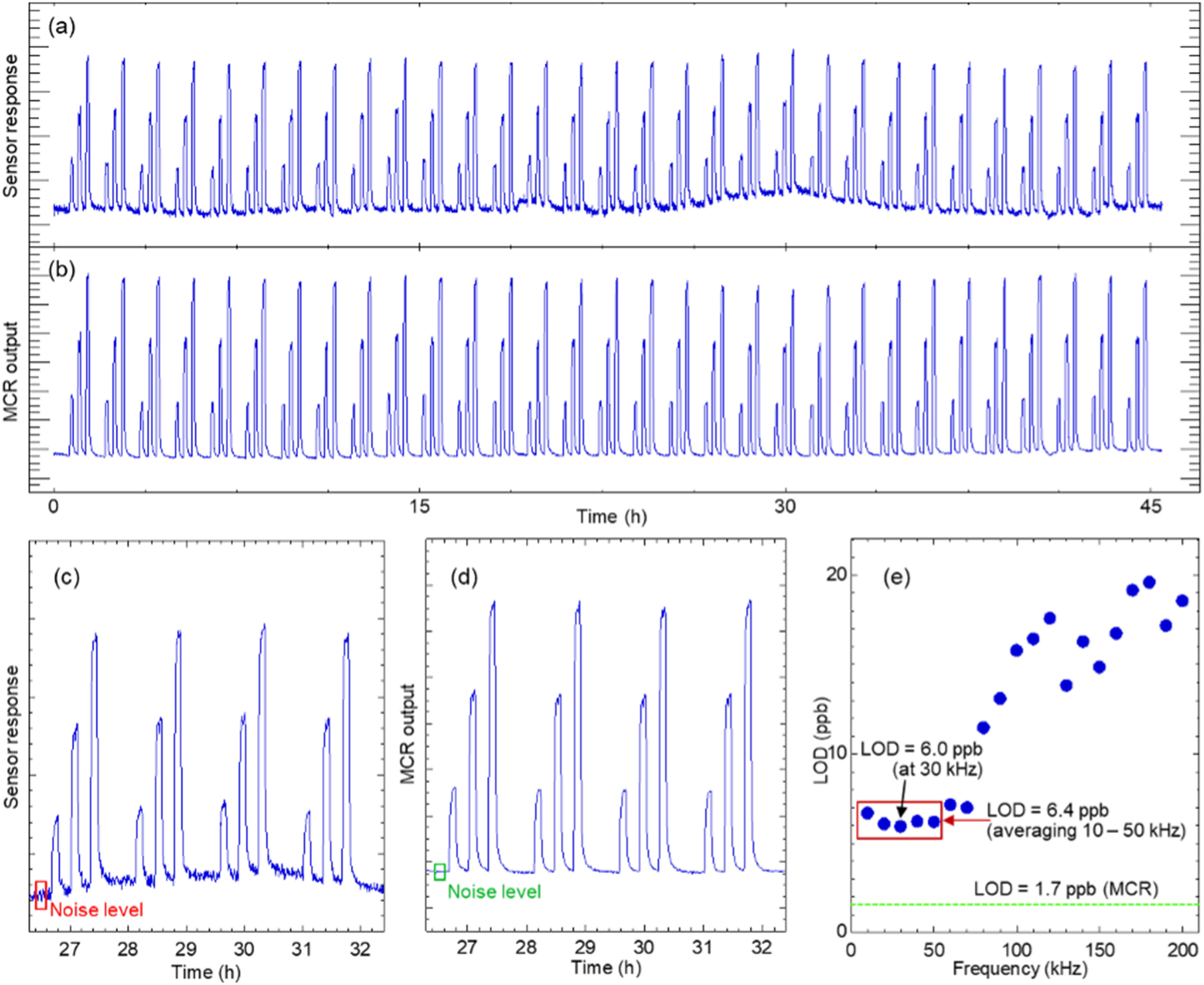
Multifrequency MCR self-correction of baseline drift of a SMOX sensing element under its dielectric excitation during multiple cycles of NO₂ exposures to 80, 160, and 240 ppb of NO₂ collected over 45 h of experiment in ambient lab conditions. (a) Sensor baseline fluctuation of raw sensor response. (b) MCR results using all operation frequencies of our ASIC impedance analyzer. (c) Relatively high sensor noise and unstable sensor baseline in raw sensor response and (d) decreased noise and improved stability of baseline upon MCR implementation (d). (e) Results of LOD determination before and after implementation of the MCR algorithm. Red and green boxes in (c and d) highlight regions (50 data points over 15 min of data acquisition) to determine sensor noise.

Figure 6.

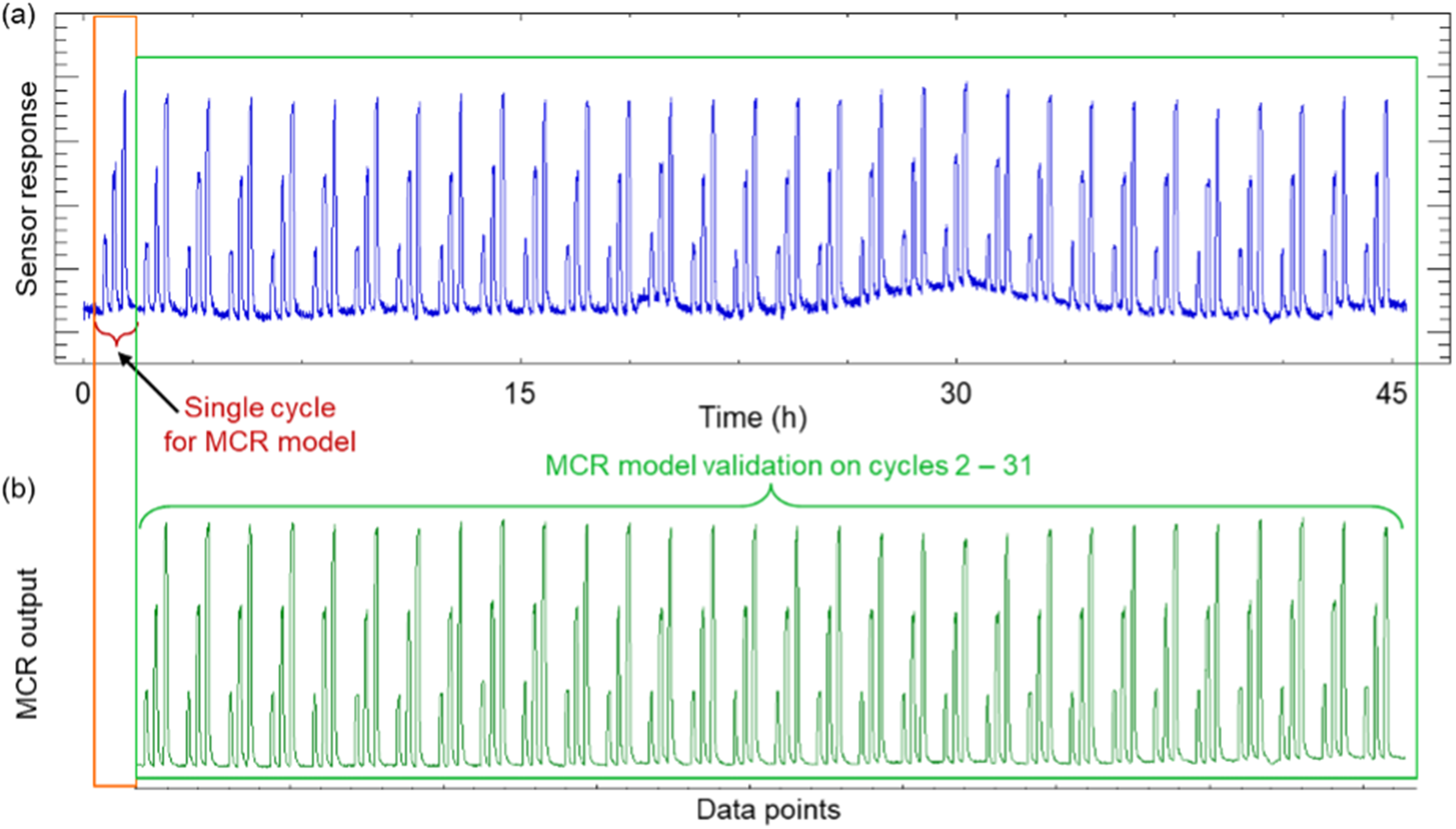
Results of application of MCR algorithm for correction of the baseline drift and reduction of noise in the SMOX sensing element under its dielectric excitation. (a) Raw response of the sensor over its 45 h of testing, with a substantial baseline drift observed after the first 15 h of the experiment. For the MCR model development of the multifrequency response of the sensor, only the first replicate of the multiple responses to NO₂ was utilized for its correction of possible baseline fluctuations. (b) The MCR algorithm preserved a steady baseline over the rest of the experiment.

The MCR analysis not only improved the baseline stability but also reduced sensor noise. Figure 5c shows four replicates of sensor response to three concentrations of NO₂ gas demonstrating the relatively high sensor noise and unstable sensor baseline that were observed during the experiment from ∼26 to ∼32.5 h of the 45 h total experiment duration. In contrast, upon implementing the MCR, the sensor noise has been decreased and the sensor baseline has become more stable over the same time period (Fig. 5d). The noise of the sensor response upon implementation of the MCR has been reduced by more than threefold.

Figure 5e depicts the results of the determination of the limit of detection (LOD) of the sensor before and after the implementation of the MCR algorithm. When measurements were done in the raw data acquisition mode, the LOD using the smallest measured analyte concentration and the noise of the baseline is highlighted with a red box in Fig. 5c. The LOD was minimal at 30 kHz (LOD = 6 ppb). The LOD did not improve by averaging the sensor response at neighbor frequencies of 10–50 kHz (LOD = 6.4 ppb). It was unexpectedly found that the implementation of the MCR algorithms has improved the LOD by 3.5–3.75 times detecting it down to 1.7 ppb of NO₂ with the noise of the baseline highlighted with a green box in Fig. 5d.

Figure 6 depicts the results of building an MCR model for the correction of the baseline drift and reduction of baseline noise in the first-order sensor. Figure 6a shows the raw sensor response over 45 h of testing where a substantial baseline drift was observed after the first 15 h of the experiment. For the MCR model development of the sensor response, only the first replicate of the multiple responses to NO₂ was utilized for its correction of possible baseline fluctuations. Figure 6b depicts that the MCR algorithm preserved a steady baseline over the rest of the experiment. Thus, by utilizing the multifrequency operation of the SMOX sensor, it was operated as the first-order device and took advantage of utilizing the MCR algorithm for automatic baseline correction and baseline noise reduction without the need for preselection of operation frequencies.

First-Order Nanostructured Photonic Gas Sensors

Principle of the First-Order Nanostructured Photonic Gas Sensors

Nanostructured photonic sensors are comprised of units that are comparable with the wavelength of interrogation light. From the initial²⁸ and detailed³¹ studies of the multigas response of natural Morpho scales, numerical analysis of optical effects from multiple vapors,³² and fabrication of bio-inspired nanostructures^32–34 (Fig. 7a), design rules of nanostructured photonic multivariable gas sensors were developed.^31–34 To evaluate the gas responses of nanostructures, optical measurements were performed in reflectance mode (Fig. 7b). The differential reflectance spectral response ΔR(λ) of the sensing nanostructure was measured upon exposure to gaseous species of interest to cancel the common features in the spectra before and during gas exposure and to accentuate the subtle differences due to gas response.^28,31 The broadband white light excitation scheme of photonic nanostructures unexpectedly provided multiwavelength drift correction as discussed in the Multiwavelength Self-Correction of Baseline Drift in the First-Order Nanostructured Photonic Gas Sensors section.

Figure 7.

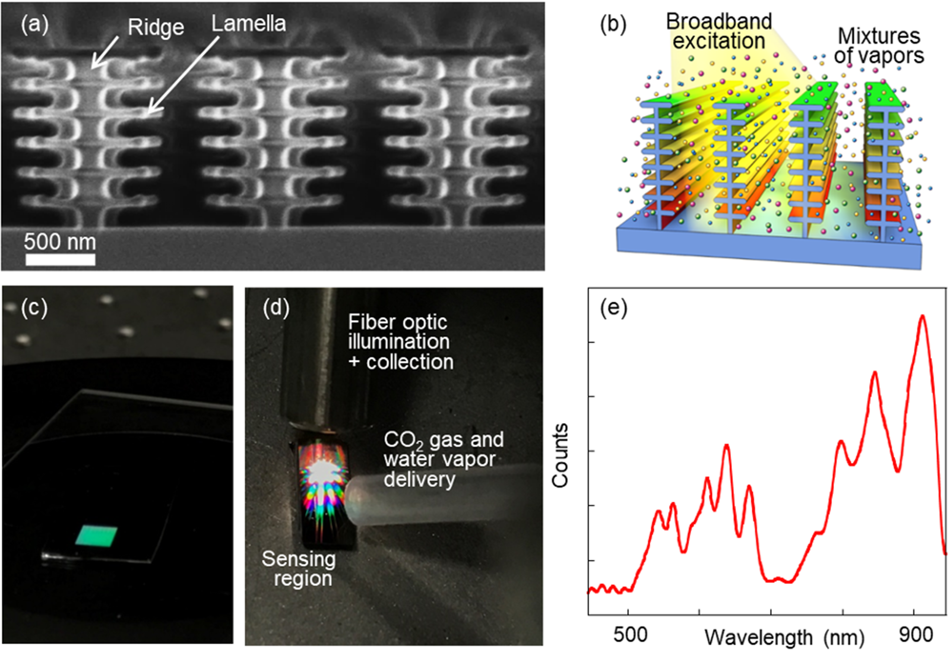
Structure-based photonic bio-inspired first-order (multivariable) gas sensors and their gas-response readout. (a) Bio-inspired nanostructures fabricated using modern lithographic tools. (b) Schematic of optical measurements in reflectance mode. (c) Reflected light image of the fabricated gas-sensing nanostructure. (d) A colored pattern of diffraction and interference of white light from the nanostructure. (e) Reflected light spectrum of the fabricated gas-sensing nanostructure in the air.

Multiwavelength Self-Correction of Baseline Drift in the First-Order Nanostructured Photonic Gas Sensors

Industrial processes require gas monitoring over broad concentration ranges. In the example illustrated here, the detection of high gas concentrations of CO₂ as a model gas of interest and mixtures of CO₂ with water vapor was performed. Figures 7c–7e show a fabricated gas-sensing nanostructured sensor and its reflectance spectrum under a white light illumination. Depending on the illumination angle, the sensor had different reflected colors, such as a blue-green (Fig. 7c). White-light illumination of the sensor produced a pattern of diffraction and interference (Fig. 7d). Its reflected light spectrum (Fig. 7e) illustrates a desired complex pattern produced from the different horizontal and vertical regions of the nanostructure.^31,32

The CO₂ gas concentrations used in these experiments were 22%, 44%, 67%, and 89%. Water vapor concentrations were measured as relative humidity (RH) values of 5% and 10% RH. A plan of an experimental cycle of exposures to CO₂, H₂O, and mixtures of CO₂ and H₂O is presented in Fig. S2 (Supplemental Material). Each step of individual CO₂ and H₂O exposures was 2 min, with 2 min between exposures. The duration of the whole experimental cycle shown in Fig. S2 (Supplemental Material) was ∼100 min. The duration of the whole experiment was ∼18 h with 3000 data points collected (∼20 s per data point).

Figure S3 (Supplemental Material) depicts examples of the responses of the sensor to CO₂, H₂O, and their mixtures at three wavelengths. As expected from the previously developed design rules for such sensors,³² the relative response of the same sensor to CO₂ and H₂O vapors was very different when probed at different wavelengths. For example, probing of the sensor response at ∼890 nm demonstrated the sensor response to 10% RH to be similar to the response to 44% of CO₂ (dotted red horizontal line in Fig. S3a, Supplemental Material). However, probing of the sensor response at ∼875 nm demonstrated the sensor response to 10% RH to be half of the response to 22% of CO₂ (dotted red horizontal line in Fig. S3b, Supplemental Material). Finally, sensor response at ∼577 nm had a very negligible response to 10% RH (dotted red horizontal line in Fig. S3c, Supplemental Material). This response diversity at different wavelengths provides an ability to differentiate between the gas of interest and interferences. Spectral responses of the sensor to CO₂ and H₂O as the differential reflectance ΔR(λ) illustrated spectral regions that exhibited suppressed responses to H₂O, around 520 and 580 nm (Fig. S4, Supplemental Material).

With over ∼18 h of the experiment, the sensor response had a noticeable wavelength-dependent baseline drift. As an example, Fig. 8 depicts the response of the sensor at four illustrative wavelengths. At one of the wavelengths (Fig. 8a), the drift was pronounced in the middle of the experiment, while at other wavelengths (Figs. 8b and 8c), the drift was pronounced at the end of the experiment. Interestingly, at some other wavelengths (Fig. 8d), the sensor response did not have a noticeable drift. Results shown in Fig. 8e illustrate that when the MCR analysis was applied to the whole data set, it corrected the baseline drift versus the original responses (Figs. 8a–8c).

Figure 8.

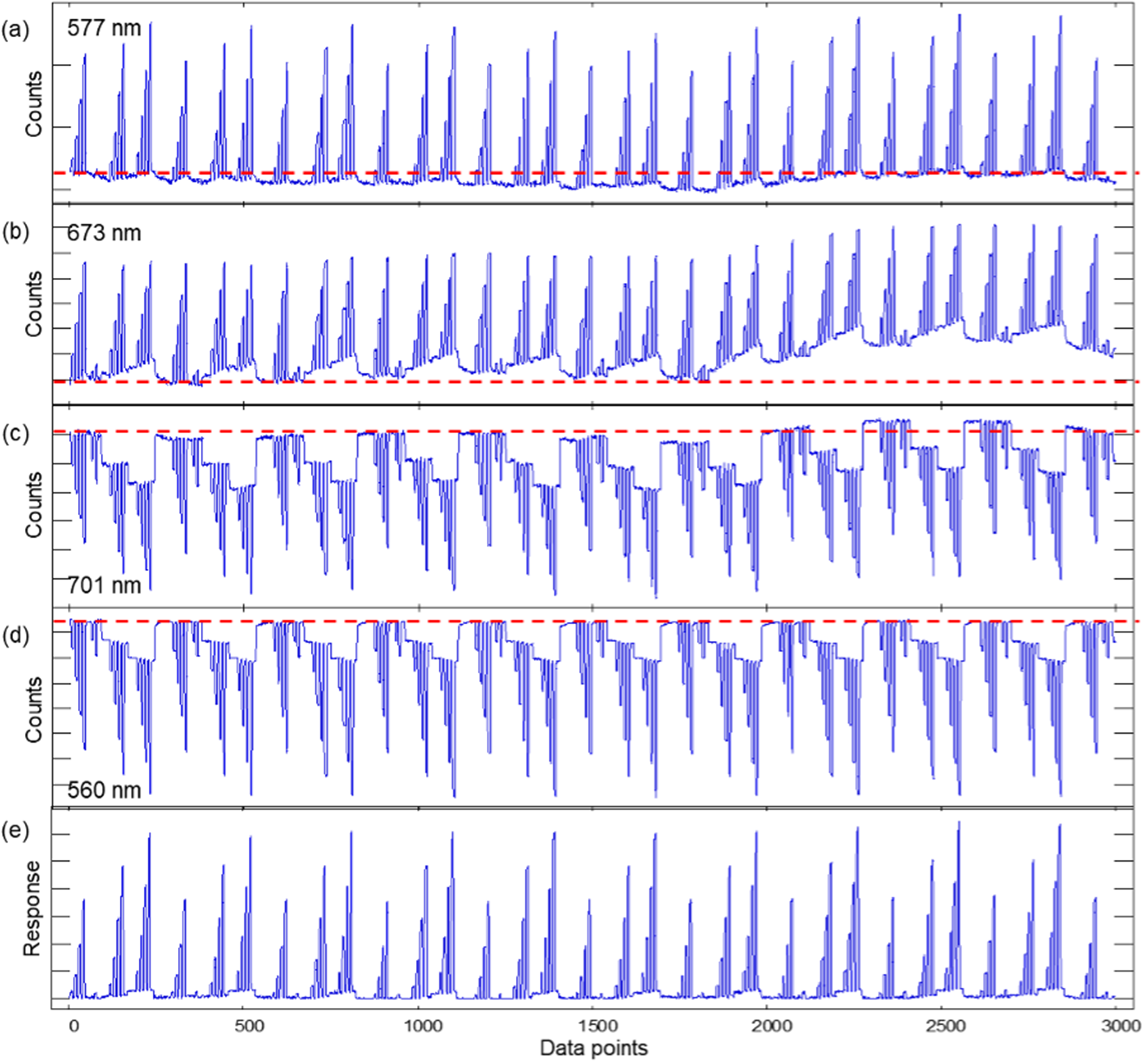
A wavelength-dependent pattern of the baseline drift of the gas-sensing nanostructure response to CO₂, H₂O vapor, and their mixtures during ∼18 h of the experiment and initial results of MCR analysis for the correction of baseline drift. (a) Drift in the middle of the experiment at 577 nm, (b, c) drift at the end of the experiment at 673 and 701 nm, and (d) no noticeable drift at 560 nm. In (a–d), a desired flat baseline is indicated as a red dashed line. (e) Results of MCR analysis for the correction of baseline drift. The duration of the whole experiment was ∼18 h with 3000 data points collected (∼20 s per data point).

In predicting gas concentrations over the whole experiment, the goal of the drift reduction was to achieve a comparable sensor performance as compared to the short-term performance of the same sensor as possible. To achieve this goal, different drift contributions in the sensor were considered. Concentrations of CO₂ in the presence of variable levels of water vapor were determined by using two types of transfer functions, both using only the first cycle of the experiment for calibration and predicting CO₂ concentrations for the rest of the replicates. The first type of transfer function did not include wavelengths with diverse effects of drift and predicted CO₂ concentrations well in the presence of H₂O vapor but did not perform well in the presence of the sensor baseline drift (Figs. 9a–9c). At the initial stages of the experiment, the transfer function worked well and rejected H₂O concentrations up to ∼2000 data points during the experiment. In the presence of drift, the prediction ability for CO₂ concentrations degraded (Fig. 9a). A comparison of the quality of predicted CO₂ at the beginning and the end of the experiment (Figs. 9b and 9c) highlights the degradation of the prediction ability of the first type of the transfer function.

Figure 9.

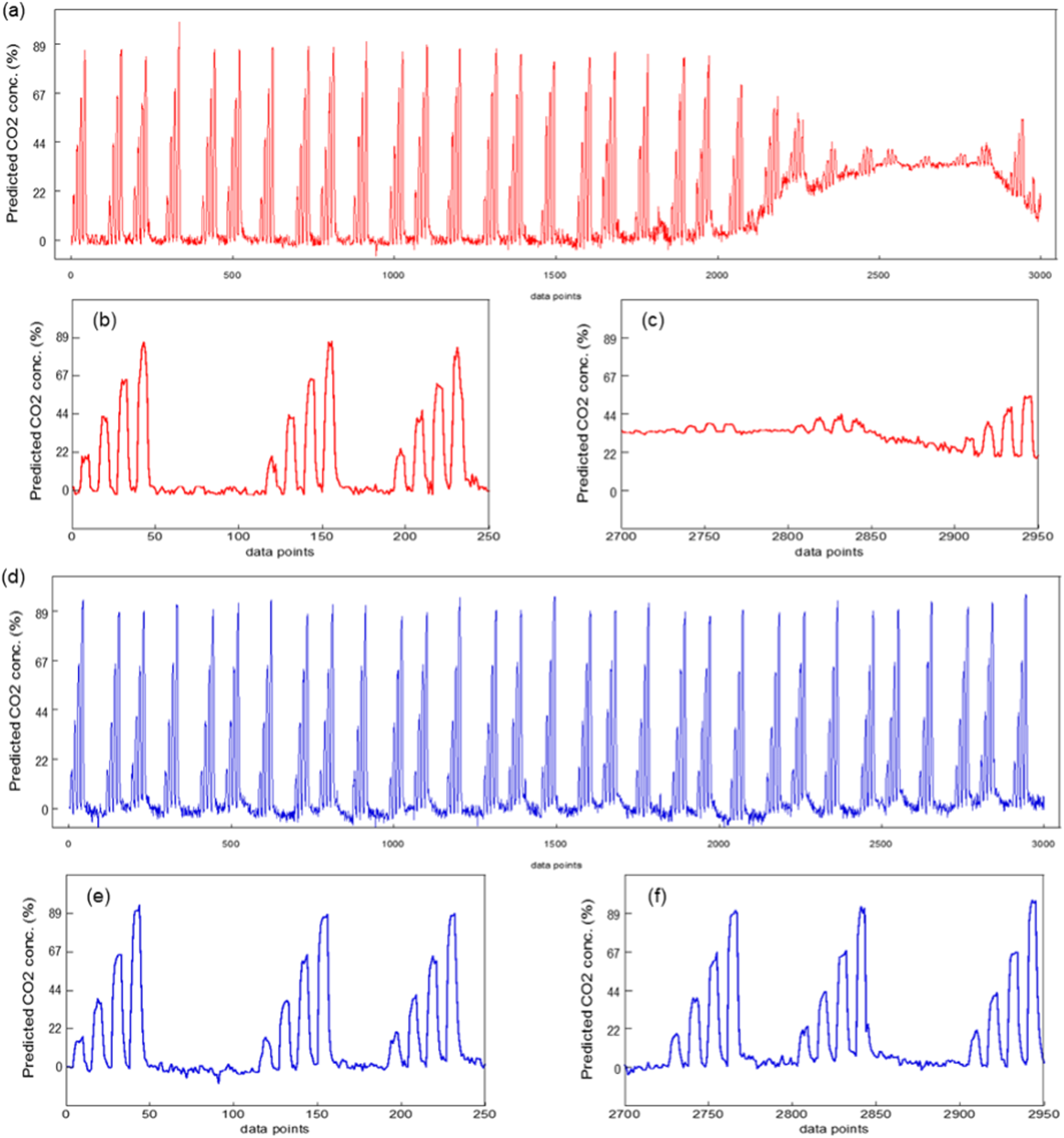
Prediction of CO₂ concentrations in the presence of H₂O vapor and uncontrolled sensor baseline drift using (a–c) the first and (d–f) second type of the transfer function. (a, d) Prediction ability for CO₂ concentrations over ∼18 h of the experiment. Quality of predicted CO₂ in the beginning (b, e) and at the end (c, f) of the experiment. The duration of the whole experiment was ∼18 h with 3000 data points collected (∼20 s per data point).

The second type of transfer function did include wavelengths with diverse effects of drift. This approach showed a dramatic desired improvement in the prediction of CO₂ concentrations (Figs. 9d–9f). At the initial stages of the experiment, the transfer function rejected H₂O concentrations. In the presence of drift, the prediction ability for CO₂ concentrations was preserved (Fig. 9d). A comparison of the quality of predicted CO₂ concentrations at the beginning and the end of the experiment (Figs. 9e and 9f) demonstrated that the prediction ability of the second type of the transfer function was unaffected by sensor drift.

Conclusion

The novelty of this study compared to previous work on the first-order individual gas sensors is threefold. First, the self-correction of baseline fluctuations of the first-order individual gas sensors was demonstrated as a general scheme across the electromagnetic spectrum with sensors operating in the RF and optical spectral regions. Second, instabilities of the baseline response were corrected by sensor operation at several regions of their independent variables of RF frequencies and optical wavelengths. Third, the MCR was demonstrated to be an attractive tool for not only the elimination of the baseline fluctuations but also for the improvement of the signal-to-noise ratio of the response of the first-order individual gas sensors.

We continue to explore methodologies available to the first-order¹⁶ analytical instruments with an inspiration of achieving a so-called second-order advantage.^38,39 The societal impact of these results is in opening opportunities for more proactive developments of diverse types of first-order gas sensors¹⁰ in diverse emerging monitoring applications, ranging from urban pollution and industrial safety to medical diagnostics and homeland protection, all of which cannot afford frequent periodic maintenance that is typical of traditional analytical instruments.

Supplemental Material

sj-docx-1-asp-10.1177_00037028231186821 - Supplemental material for First-Order Individual Gas Sensors as Next Generation Reliable Analytical Instruments

Supplemental material, sj-docx-1-asp-10.1177_00037028231186821 for First-Order Individual Gas Sensors as Next Generation Reliable Analytical Instruments by Radislav A. Potyrailo, Brian Scherer, Baokai Cheng, Majid Nayeri, Shiyao Shan, Janell Crowder, Richard St-Pierre, Joleyn Brewer and Renner Ruffalo in Applied Spectroscopy

Footnotes

Acknowledgments

This work is dedicated to Professor Gary Hieftje, the mentor and inspiration to R.A.P. in his journey in scientific innovations in analytical instrumentation and bringing these innovations to end-users. R.A.P. is proud to be a part of the Scientific Family Tree of Hieftje Research Group as his PhD student no. 45.

Declaration of Conflicting Interests

The author(s) declared no potential conflicts of interest with respect to the research, authorship, and/or publication of this article.

Funding

The author(s) disclosed receipt of the following financial support for the research, authorship, and/or publication of this article: The work on RF gas sensors was performed in part with funding from U.S. Government under Other Transaction number W15QKN-18-9-1004 between the CWMD Consortium and the Government. The work on photonic gas sensors was performed in part with funding from the U.S. Department of Energy under Award Number DE-FE0027918. The US Government is authorized to reproduce and distribute reprints for Governmental purposes, notwithstanding any copyright notation thereon. Neither the U.S. Government nor any agency thereof, nor any of their employees, makes any warranty, express or implied, or assumes any legal liability or responsibility for the accuracy, completeness, or usefulness of any information, apparatus, product, or process disclosed, or represents that its use would not infringe privately owned rights. Reference herein to any specific commercial product, process, or service by trade name, trademark, manufacturer, or otherwise does not necessarily constitute or imply its endorsement, recommendation, or favoring by the U.S. Government or any agency thereof. The views, opinions, and conclusions contained herein are those of the authors and should not be interpreted as necessarily representing the official policies or endorsements, either expressed or implied, of the U.S. Government or any agency thereof.

ORCID iDs

Radislav A. Potyrailo

Brian Scherer

Supplemental Material

All supplemental material mentioned in the text is available in the online version of the journal.

References

Kulkarni

G.S.

Reddy

Zhong

Fan

. “Graphene Nanoelectronic Heterodyne Sensor for Rapid and Sensitive Vapour Detection”. Nat. Commun. 2014. 5(1): 4376. 10.1038/ncomms5376

Luong

H.M.

Pham

M.T.

Guin

, et al. “Sub-Second and ppm-Level Optical Sensing of Hydrogen Using Templated Control of Nano-Hydride Geometry and Composition”. Nat. Commun. 2021. 12(1): 2414. 10.1038/s41467-021-22697-w

Janata

. Principles of Chemical Sensors. New York: Springer, 2009.

Ljunggren

. Means for and Method of Detecting the Presence of Carbon Monoxide. US Patent 1891429A. Filed 1931. Issued 1932.

Taguchi

. Method for Making a Gas-Sensing Element. US Patent 3625756A. Filed 1969. Issued 1971.

Lewis

Edwards

. “Validate Personal Air-Pollution Sensors”. Nature. 2016. 535(7610): 29–31. 10.1038/535029a

Austen

. “Environmental Science: Pollution Patrol”. Nature. 2015. 517(7533): 136–138. 10.1038/517136a

Chai

Zheng

Liu

, et al. “Stability of Metal Oxide Semiconductor Gas Sensors: A Review”. IEEE Sens. J. 2022. 22(6): 5470–5481. 10.1109/JSEN.2022.3148264

Müller

Sberveglieri

. “Origin of Baseline Drift in Metal Oxide Gas Sensors: Effects of Bulk Equilibration”. Chemosensors. 2022. 10(5): 171. 10.3390/chemosensors10050171

10.

Potyrailo

R.A.

. “Multivariable Sensors for Ubiquitous Monitoring of Gases in the Era of Internet of Things and Industrial Internet”. Chem. Rev. 2016. 116(19): 11877–11923. 10.1021/acs.chemrev.6b00187

11.

Persaud

Dodd

. “Analysis of Discrimination Mechanisms in the Mammalian Olfactory System Using a Model Nose”. Nature. 1982. 299(5881): 352–355. 10.1038/299352a0

12.

Zaromb

Stetter

J.R.

. “Theoretical Basis for Identification and Measurement of Air Contaminants Using an Array of Sensors Having Partly Overlapping Selectivities”. Sens. Actuators. 1984. 6(4): 225–243. 10.1016/0250-6874(84)85019-2

13.

Carey

W.P.

Beebe

K.R.

Sanchez

Geladi

Kowalski

B.R.

. “Chemometric Analysis of Multisensor Arrays”. Sens. Actuators. 1986. 9(3): 223–234. 10.1016/0250-6874(86)80023-3

14.

Tonezzer

D.T.T.

Van Duy

Duc Hoa

, et al. “Electronic Noses Based on Metal Oxide Nanowires: A Review”. Nanotechnol. Rev. 2022. 11(1): 897–925. 10.1515/ntrev-2022-0056

15.

Bax

Prudenza

Gaspari

Capelli

, et al. “Drift Compensation on Electronic Nose Data for Non-Invasive Diagnosis of Prostate Cancer by Urine Analysis”. iScience. 2022. 25(1): 103622. 10.1016/j.isci.2021.103622

16.

Booksh

K.S.

Kowalski

B.R.

. “Theory of Analytical Chemistry”. Anal. Chem. 1994. 66(15): 782A–791A. 10.1021/ac00087a718

17.

Williams

Kilaru

Snyder

Kaufman

, et al. “Air Sensor Guidebook”. Washington, DC: U.S. Environmental Protection Agency, 2014.

18.

Lewis

A.C.

von Schneidemesser

Peltier

R.E.

. “Low-Cost Sensors for the Measurement of Atmospheric Composition: Overview of Topic and Future Applications”. 2018. https://www.ccacoalition.org/en/resources/low-cost-sensors-measurement-atmospheric-composition-overview-topic-and-future [accessed Jun 21 2023].

19.

Rai

A.C.

Kumar

Pilla

Skouloudis

A.N.

, et al. “End-User Perspective of Low-Cost Sensors for Outdoor Air Pollution Monitoring”. Sci. Total Environ. 2017. 607(December): 691–705. 10.1016/j.scitotenv.2017.06.266.

20.

Potyrailo

R.A.

Morris

W.G.

. “Multianalyte Chemical Identification and Quantitation Using a Single Radio Frequency Identification Sensor”. Anal. Chem. 2007. 79(1): 45–51. 10.1021/ac061748o

21.

Potyrailo

R.A.

Morris

W.G.

Sivavec

Tomlinson

H.W.

, et al. “RFID Sensors Based on Ubiquitous Passive 13.56 MHz RFID Tags and Complex Impedance Detection”. Wireless Commun. Mobile Comput. 2009. 9(10): 1318–1330. 10.1002/wcm.711

22.

Potyrailo

R.A.

Surman

Lee

, et al. “Development of Radio-Frequency Identification Sensors Based on Organic Electronic Sensing Materials for Selective Detection of Toxic Vapors”. J. Appl. Phys. 2009. 106(12): 124902. 10.1063/1.3247069

23.

Potyrailo

R.A.

Burns

Surman

Lee

D.J.

McGiniss

. “Multivariable Passive RFID Vapor Sensors: Roll-to-Roll Fabrication on a Flexible Substrate”. Analyst. 2012. 137(12): 2777–2781. 10.1039/C2AN16278D

24.

Nagraj

Slocik

J.M.

Phillips

D.M.

Kelley-Loughnane

, et al. “Selective Sensing of Vapors of Similar Dielectric Constants Using Peptide-Capped Gold Nanoparticles on Individual Multivariable Transducers”. Analyst. 2013. 138(15): 4334–4339. 10.1039/C3AN00088E

25.

Potyrailo

R.A.

Surman

. “A Passive Radio-Frequency Identification (RFID) Gas Sensor with Self-Correction Against Fluctuations of Ambient Temperature”. Sens. Actuators, B. 2013. 185: 587–593. 10.1016/j.snb.2013.04.107.

26.

Potyrailo

R.A.

. “Multivariable Gas Sensors: Delivering Needed Selectivity and Stability for Modern Applications”. Tutorial presented at: IEEE SENSORS. New Delhi, India; October 28–31, 2018. https://2018.ieee-sensorsconference.org/tutorials [accessed Jun 21 2023].

27.

Potyrailo

R.A.

Sexton

, et al. “Extraordinary Performance of Semiconducting Metal Oxide Gas Sensors Using Dielectric Excitation”. Nat. Electron. 2020. 3(5): 280–289. 10.1038/s41928-020-0402-3

28.

Potyrailo

R.A.

Ghiradella

Vertiatchikh

Dovidenko

, et al. “Morpho Butterfly Wing Scales Demonstrate Highly Selective Vapour Response”. Nat. Photonics. 2007. 1(2): 123–128. 10.1038/nphoton.2007.2

29.

Potyrailo

R.A.

Ding

Butts

M.D.

Genovese

S.E.

Deng

. “Selective Chemical Sensing Using Structurally Colored Core-Shell Colloidal Crystal Films”. IEEE Sensors J. 2008. 8(6): 815–822. 10.1109/JSEN.2008.923191

30.

Potyrailo

R.A.

Larsen

Riccobono

. “Detection of Individual Vapors and Their Mixtures Using a Selectivity-Tunable Three-Dimensional Network of Plasmonic Nanoparticles”. Angew. Chem. Int. Ed. 2013. 52(39): 10360–10364. 10.1002/anie.201305303

31.

Potyrailo

R.A.

Starkey

T.A.

Vukusic

Ghiradella

, et al. “Discovery of the Surface Polarity Gradient on Iridescent Morpho Butterfly Scales Reveals a Mechanism of Their Selective Vapor Response”. Proc. Natl. Acad. Sci. U.S.A. 2013. 110(39): 15567–15572. 10.1073/pnas.1311196110

32.

Potyrailo

R.A.

Bonam

R.K.

Hartley

J.G.

Starkey

T.A.

, et al. “Towards Outperforming Conventional Sensor Arrays With Fabricated Individual Photonic Vapour Sensors Inspired by Morpho Butterflies”. Nat. Commun. 2015. 6(1): 7959. 10.1038/ncomms8959

33.

Potyrailo

R.A.

Karker

Carpenter

M.A.

Minnick

. “Multivariable Bio-Inspired Photonic Sensors for Non-Condensable Gases”. J. Opt. 2018. 20(2): 024006. 10.1088/2040-8986/aa9ecf

34.

Potyrailo

R.A.

Brewer

Cheng

Carpenter

M.A.

, et al. “Bio-Inspired Gas Sensing: Boosting Performance with Sensor Optimization Guided by ‘Machine Learning’”. Faraday Discuss. 2020. 223: 161–182. 10.1039/D0FD00035C.

35.

Potyrailo

R.A.

Nagraj

Surman

Boudries

, et al. “Wireless Sensors and Sensor Networks for Homeland Security Applications”. Trends Anal. Chem. 2012. 40: 133–145. 10.1016/j.trac.2012.07.013.

36.

Potyrailo

R.A.

Naik

R.R.

. “Bionanomaterials and Bioinspired Nanostructures for Selective Vapor Sensing”. Annu. Rev. Mater. Res. 2013. 43(1): 307–334. 10.1146/annurev-matsci-071312-121710

37.

Potyrailo

R.A.

. “Toward High Value Sensing: Monolayer-Protected Metal Nanoparticles in Multivariable Gas and Vapor Sensors”. Chem. Soc. Rev. 2017. 46(17): 5311–5346. 10.1039/c7cs00007c

38.

Chiappini

F.A.

Gutierrez

Goicoechea

H.C.

Olivieri

A.C.

. “Interference-Free Calibration with First-Order Instrumental Data and Multivariate Curve Resolution. When and Why?”. Anal. Chim. Acta. 2021. 1161: 338465. 10.1016/j.aca.2021.338465.

39.

Mazivila

S.J.

Santos

J.L.

. “A Review on Multivariate Curve Resolution Applied to Spectroscopic and Chromatographic Data Acquired During the Real-Time Monitoring of Evolving Multi-Component Processes: From Process Analytical Chemistry (PAC) to Process Analytical Technology (PAT)”. TrAC, Trends Anal. Chem. 2022. 157(December): 116698.

40.

The Nobel Prize. “All Nobel Prizes”. https://www.nobelprize.org/prizes/lists/all-nobel-prizes/ [accessed Jun 21 2023].

41.

2B Technologies. “Ozone Monitor Scrubberless Dual Beam”. https://twobtech.com/docs/manuals/model_211_revH-3.pdf [accessed Jun 21 2023].

42.

Yokagawa Electric Corporation. “Model IR400 Infrared Gas Analyzer User Manual”. https://web-material3.yokogawa.com/GS11G02N01-01E.pdf [accessed Jun 21 2023].

43.

Thermo Scientific. “Model 43i Pulsed Fluorescence SO2 Analyzer User Manual, Thermo Fisher Scientific”. https://assets.thermofisher.com/TFS-Assets/LSG/manuals/EPM-manual-Model%2043i.pdf [accessed Jun 21 2023].

44.

U.S. Environmental Protection Agency (EPA). “Reference Method for the Determination of Nitrogen Dioxide in the Atmosphere (Chemiluminescence), EPA Quality Assurance Handbook”. https://www3.epa.gov/ttnamti1/files/ambient/pm25/qa/no2.pdf [accessed Jun 21 2023].

45.

Scientific Engineering Response and Analytical Services (SERAS). “Standard Operating Procedures: Operation of the Hapsite Field Portable Gas Chromatograph/Mass Spectrometer (GC/MS) (Triad GC/MS Based on EPA/TO-15A)”. https://clu-in.org/download/ert/1726-r00.pdf [accessed Jun 21 2023].

46.

Smiths Detection, Inc. “LCD 3.2E (JCAD) Manual”. London: Smiths Detection, Inc., 2022. https://www.manualslib.com/manual/2074305/Smiths-Detection-Lcd-3-3.html [accessed Jun 21 2023].

47.

Flach

P.A.

. “ROC Analysis”. In: Sammut

Webb

G.I.

, editors. Encyclopedia of Machine Learning. Boston: Springer, 2010. Pp. 869–875.

48.

The Mathworks, Inc., “Detector Performance Analysis Using ROC Curves”. 2023. https://www.mathworks.com/help/phased/ug/detector-performance-analysis-using-roc-curves.html;jsessionid=6c73c286a6766c9b215942b602ee [accessed Jun 21 2023].

49.

Potyrailo

R.A.

Wroczynski

R.J.

Lemmon

J.P.

, et al. “Multivariate Tools for Real-Time Monitoring and Optimization of Combinatorial Materials and Process Conditions”. In: Yan

, editor. Analysis and Purification Methods in Combinatorial Chemistry. Hoboken. New Jersey: Wiley-Interscience, 2004. Pp. 87–123. 10.1002/0471531979.ch5

50.

de Juan

Tauler

. “Multivariate Curve Resolution: 50 Years Addressing the Mixture Analysis Problem: A Review”. Anal. Chim. Acta. 2021. 1145(February): 59–78. 10.1016/j.aca.2020.10.051.

51.

Izawa

Ulmer

Staerz

Weimar

Barsan

. “Application of SMOX-Based Sensors”. In: Barsan

Schierbaum

, editors. Gas Sensors Based on Conducting Metal Oxides: Basic Understanding, Technology, and Applications. Amsterdam: Elsevier, 2019. Pp. 217–257. 10.1016/B978-0-12-811224-3.00005-6

52.

Tao

. “Challenges and Promises of Metal Oxide Nanosensors”. ACS Sens. 2019. 4(4): 780–780. 10.1021/acssensors.9b00622

53.

Ingle

J.D.

Jr. Crouch

S.R.

. Spectrochemical Analysis. Englewood Cliffs, New Jersey: Prentice Hall, 1988.

Supplementary Material

Please find the following supplemental material available below.

For Open Access articles published under a Creative Commons License, all supplemental material carries the same license as the article it is associated with.

For non-Open Access articles published, all supplemental material carries a non-exclusive license, and permission requests for re-use of supplemental material or any part of supplemental material shall be sent directly to the copyright owner as specified in the copyright notice associated with the article.

0.00 MB

0.46 MB