Detection of Chylous Plasma Based on Machine Learning and Hyperspectral Techniques

Abstract

Chylous blood is the main cause of unqualified and scrapped blood among volunteer blood donors. Therefore, a diagnostic method that can quickly and accurately identify chylous blood before donation is needed. In this study, the GaiaSorter “Gaia” hyperspectral sorter was used to extract 254 bands of plasma images, ranging from 900 nm to 1700 nm. Four different machine learning algorithms were used, including decision tree, Gaussian Naive Bayes (GaussianNB), perceptron, and stochastic gradient descent models. First, the preliminary classification accuracies were compared with the original data, which showed that the effects of the decision tree and GaussianNB models were better; their average accuracies could reach over 90%. Then, the feature dimension reduction was performed on the original data. The results showed that the effects of the decision tree were better with a classification accuracy of 93.33%. the classification of chylous plasma using different chylous indices suggested that the accuracies of the decision trees model both before and after the feature dimension reductions were the best with over 80% accuracy. The results of feature dimension reduction showed that the characteristic bands corresponded to all kinds of plasma, thereby showing their classification and identification potential. By applying the spectral characteristics of plasma to medical technology, this study suggested a rapid and effective method for the identification of chylous plasma and provided a reference for the blood detection technology to achieve the goal of reducing wasting blood resources and improving the work efficiency of the medical staff.

Graphical abstract

This is a visual representation of the abstract.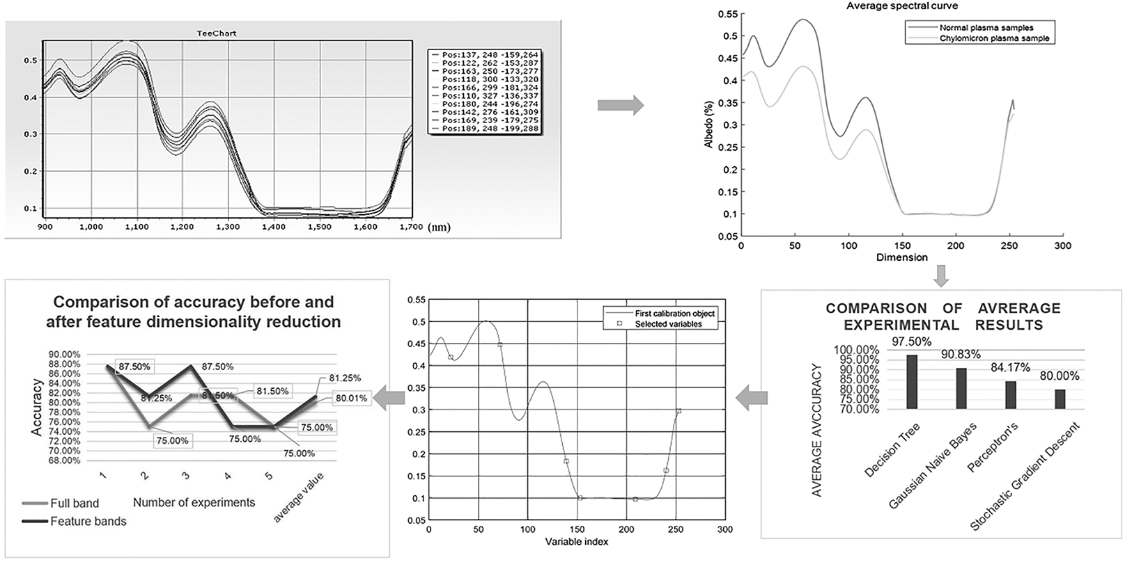

Keywords

Chylous plasma hyperspectral techniques decision tree Gaussian Naive Bayes GaussianNB‌perceptrons stochastic gradient descent

Introduction

Currently, the lifespan of modern people is constantly improving, but the lifestyle is getting unhealthy. A large amount of high-fat content food is being consumed in daily life, which in combination with a lack of exercise results in a large amount of fat accumulation in the body,¹ thereby increasing the fat content in blood.² The increase in blood fat contents makes the blood plasma appear milky white or cloudy, thereby forming chylous blood.³ Chylous blood should not be used for clinical purposes.⁴ Its injection into the patients causes adverse reactions, such as allergy, fever, and fat embolism,⁵ thereby further harming the patient. Therefore, a convenient and fast method for differentiating between chylous and normal healthy blood should be urgently developed.⁶

Currently, the direct and accurate method for differentiating between chylous and normal healthy blood includes the detection of plasma components and identification of chylous blood by components. Although the results are very accurate, it is a time-consuming process. The detection of a single component takes about 5 min, thereby greatly reducing the detection efficiency and failing to meet the current detection requirements.⁷ However, the detection methods for chylous blood, which are based on machine vision and image analysis, have also been widely used and can improve detection efficiency. However, the detection method based on image analysis is limited to the calculation of image grayscale values and can easily be affected by background noise, resulting in inaccurate detection results.⁸ Hyperspectral imaging is a combination of imaging and spectral technologies and is based on a very large number of narrow-band imaging data. It detects the two-dimensional geometric space and one-dimensional spectral information of the target object and obtains continuous and narrow-band imaging data with high spectral resolution.⁹ Therefore, this technology has near-continuous spectral information, and after spectral reflectance reconstruction, the hyperspectral images can obtain the near-continuous spectral reflectance curve of the measured sample; this data matches the actual measured value of the object.¹⁰ The hyperspectral data can be used to determine the absorption spectral characteristics of a sample, thereby accurately determining the components of the sample.¹¹ Visible light and near-infrared spectroscopy has been shown to human blood to identify effectively, and studies of the reflection spectrum are being used to identify human blood.¹²

Currently, studies on the use of hyperspectral imaging technology for the identification of chylous blood are lacking. In this study, hyperspectral technology was used to identify the chylous plasma and the detection results could not be easily disturbed by external noise, thereby improving the detection efficiency. A full-band hyperspectral sorter was used to obtain the rich spectral data from plasma samples as well as their reflectance to each band. The normal plasma and chylous plasma were distinguished by the differences in their reflectance, and the chylous plasmas with different chylous indices (CIs) were further divided. A method for detecting blood spots in light brown eggshells on the basis of hyperspectral transmission image is reported. Five feature wavelengths of intact eggs selected by the successive projections algorithm and three absorption peak locations of eggshells were regarded as characteristic bands to obtain better results.¹³ The feature dimensions of the data were reduced, and the characteristic bands were selected to classify the samples, which greatly reduced the calculation amount and detection time, thereby obtaining an accurate classification effect and greatly improving the detection efficiency. Using hyperspectral imaging technology for the identification of chylous blood does not require medical reagents and other instruments to identify the blood components. Moreover, there is no need to worry about blood contamination caused by sample collection. The medical staff can easily perform numerous blood identification tests, thereby greatly reducing the waste of material and human resources.

Experimental

Materials and Methods

A GaiaSorter (Specim) (Figure S1, Supplemental Material) was used in this study, which is a core component of the Gaia hyperspectral sorting instrument and a high-performance ground object hyperspectral scanning system with a wavelength, covering 400–1000 nm and 900–1700 nm.

Data Collection Methods

In the first step, a total of eight bags of plasma were used for sampling, including four chylous and four healthy plasma samples, which were collected and vacuum-packed in Ganzhou Central Blood Station, Ganzhou, China. In the second step, the plasma samples with different CIs, including 12 bags of plasma with CIs of 7, 8, and 9, were collected, as shown in Figure S2 (Supplemental Materials).

On the left, the numbers 2–5 and 6–9 represent the normal and chylous plasma samples, respectively. On the right, the first one is a normal plasma sample while the other three are chylous plasma samples with CIs represented as numbers 7, 8, and 9.

Data Pre-Processing

Before data acquisition, the instrument was turned on and preheated for 30 min to eliminate the effects of baseline drift. Then, the forward and backward speeds of the mobile radio were set to 1.6 and 2 cm/s, respectively. Furthermore, the camera exposure time and region of interest band were set to 19.1 ms and 895.91–1700.97 nm, respectively. The plasma samples were manually placed on a mobile platform for collection. 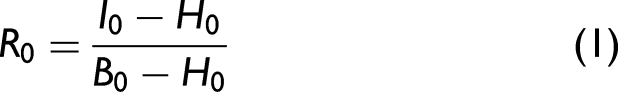The black and white calibration was performed to eliminate the effects of uneven illumination and dark current.¹⁴ The lens cover was put on to collect the blackboard “H” and removed to collect whiteboard “B,” obtaining the original data image “I.” The black and white calibrations were calculated according to Eq. 1:

R_{0} = \frac{I_{0} - H_{0}}{B_{0} - H_{0}}

(1)

where R₀, I₀, H₀, and B₀ were the calibrated, original, blackboard, and whiteboard data, respectively. The sample point data were selected from the images after calibration.

Due to the small amount of plasma sample data, 10 sample points need to be collected for one plasma sample. Moreover, the sample is a viscous fluid packed in vacuum, which cannot make the plasma volume at each position the same. Therefore, the method of regional average is adopted to approximately achieve more accurate sample point data. For the random regions, their average data were selected as sample point data. The plasma distribution in the selected regions was relatively uniform, as shown in Figure S3 (Supplemental Material).

A first data set was built using the 80 collected samples, which were randomly divided into a training set (70%) and test set (30%) and labeled as “1” and “0” for normal and chylous plasma samples, respectively. The second collected 120 plasma samples were randomly divided into a training set (80%) and a test set (20%). The samples with CIs of 7, 8, and 9 were labeled as “0”, “1”, and “2”, respectively.

Data Analysis Methods and Evaluation

Machine Learning Algorithms

In this study, four machine learning algorithms were used to test the model with the collected hyperspectral data sets, and the most suitable model was selected by comparing the results. The models included decision tree,¹⁵ Gaussian Naive Bayes (GaussianNB),¹⁶ perceptron,¹⁷ and stochastic gradient descent.¹⁸

Decision Tree Model

The decision tree model is a tree diagram, which consists of decision points, survey points, and results. The benefit values of various schemes under different conditions were solved graphically by taking the maximum expected revenue or minimum expected cost as the decision criteria, and the decision was made by comparison. This experimental model used the feature weight calculation method based on Gini gain. The specific methods were as follows. First, the increase in impurity in the feature fork was calculated in each tree. Second, if there were multiple trees, the mean value of impurity improvement in each feature was calculated. Third, the mean value was used as the feature weight.

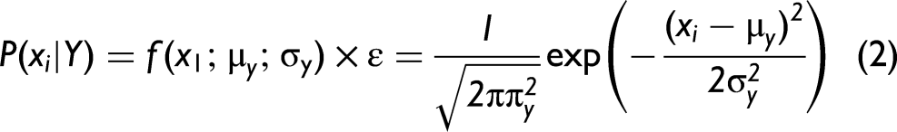
Gaussian Naive Bayes (GaussianNB)

The GaussianNB model estimates the conditional probability value of each category in each feature using the Gaussian distribution of the probability of obtaining eigenvalue X_i. For any value of Y, Bayes aims to solve for the maximum P(X_i|Y) to identify the category to which the samples are closer under different labels. GaussianNB was calculated according to Eq. 2:

P (x_{i} | Y) = f (x_{1}; μ_{y}; σ_{y}) \times ε = \frac{1}{\sqrt{2 {π π}_{y}^{2}}} \exp (- \frac{{(x_{i} - μ_{y})}^{2}}{2 σ_{y}^{2}})

(2)

where μ _y and σ _y ² were the expectation and variance of the Gaussian distribution.

Perceptron

Perceptron corresponds to a separated hyperplane, which divides the features into positive and negative categories in the feature space. Perceptron is represented as a mapping function from the input space to the output space, as given in Eq. 3:

f (x) = sign (w x + b)

(3)

where w and b are the model parameters of perceptron and called weight or weight vector and bias, respectively; w x was the inner product of w and x; and the sign represented the sign function, as given in Eq. 4:

sign = {\begin{matrix} + 1, x \underline{>} 0 \\ - 1, x \underline{<} 0 \end{matrix}

(4)

Stochastic Gradient Descent

The stochastic gradient descent model is an effective and simple method for the discriminant learning of linear classifiers under the convex loss function. The SGDClassifier was used to execute a common stochastic gradient descent program for obtaining a well-fitted model. Then, the fitted model was used to predict the new value.

Feature Dimensionality Reduction Method

The collected hyperspectral data included a data set with 254 bands. There might be a large amount of redundant data in this high-dimensional data; this redundancy was avoided by reducing the feature dimension using the continuous projection method. The continuous projection algorithm is a forward iterative search method,¹⁹ starting from the wavelength, and adding a new variable in each iteration until the number of selected variables reaches the set value of N. The algorithm is performed in the following steps:

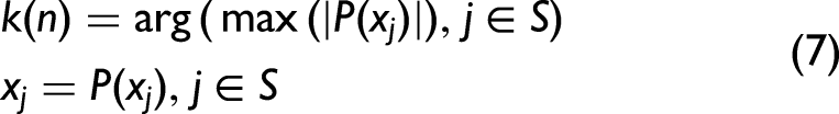
The initial iteration vector and number of variables to be extracted were denoted as x_k₍₀₎ and N, respectively, and the spectral matrix was J columns.

One column of the special matrix was selected and assigned as x_j, denoting x_k₍₀₎.

The unselected column vectors were denoted as:

S = {j, 1 \underline{<} j \underline{<} J \notin {k (0) \leftrightarrow k (n - 1)}}

(5)

The projection of x_j on the remaining column vectors was calculated.

P (x_{j}) = x_{j} - (x_{j}^{T} - x_{k (n - 1)}) x_{k (n - 1)} (x_{k (n - 1)}^{T} - x_{k (n - 1)})^{- 1}

(6)

The spectral wavelength of the maximum projection vector was extracted.

\begin{aligned} k (n) = \arg (max (| P (x_{j}) |), j \in S) \\ x_{j} = P (x_{j}), j \in S \end{aligned}

(7)

Steps (iii), (iv), and (v) were repeated for n = n + 1 and n < N.

After the wavelength combination was obtained corresponding to k(0) and N in each cycle, the prediction model was established, and the x_k₍₀₎ and N corresponding to the minimum root mean square error (RMSE) were taken.

Model Evaluation Method

In this study, two methods were used for the evaluation of the model. One method drew the receiver operating characteristic (ROC) curve of the model and calculated the area under the ROC (AUC) values,²⁰ while the other calculated the recall rate and compared the model performance to evaluate the model.²¹

The ROC curve of the model was drawn, and the evaluation method of AUC value was calculated, which was suitable for the performance evaluation of normal and chylous plasma classification models.

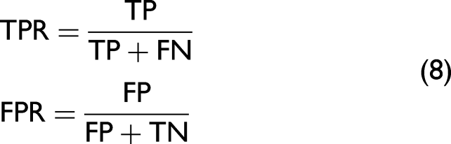
A new set of false positive rates (FPRs) and true positive rates (TPRs) were obtained by selecting the different thresholds each time. The ROC curve could be drawn by taking the FPRs as the abscissa and TPRs as the ordinate. The TPRs and FPRs were calculated as given in Eq. 8:

\begin{aligned} TPR = \frac{TP}{TP + FN} \\ FPR = \frac{FP}{FP + TN} \end{aligned}

(8)

where TP and TN represented correctly classified positive and negative samples, respectively, and FN and FP represented incorrectly classified positive and negative samples, respectively.

In the second method, for calling the model recall function, the default value of the parameter “average” was changed to “Macro”. This evaluation method was applied to models for differentiating between the different CIs. This method first calculated the recall for each category, and then calculated the average value as the final recall of the model (Recall), which was calculated as given in Eq. 9:

Re call = (\frac{T P_{0}}{T P_{0} + F N_{0}} + \frac{T P_{1}}{T P_{1} + F N_{1}} + \frac{T P_{2}}{T P_{2} + {FN}_{2}}) \times \frac{1}{3}

(9)

Results and Discussion

Separability of Plasma Samples

The spectral data of 80 sample points were collected and exported to tables, and the spectral curves of various samples were respectively viewed, as shown in Figures 1a and 1b.

Figure 1.

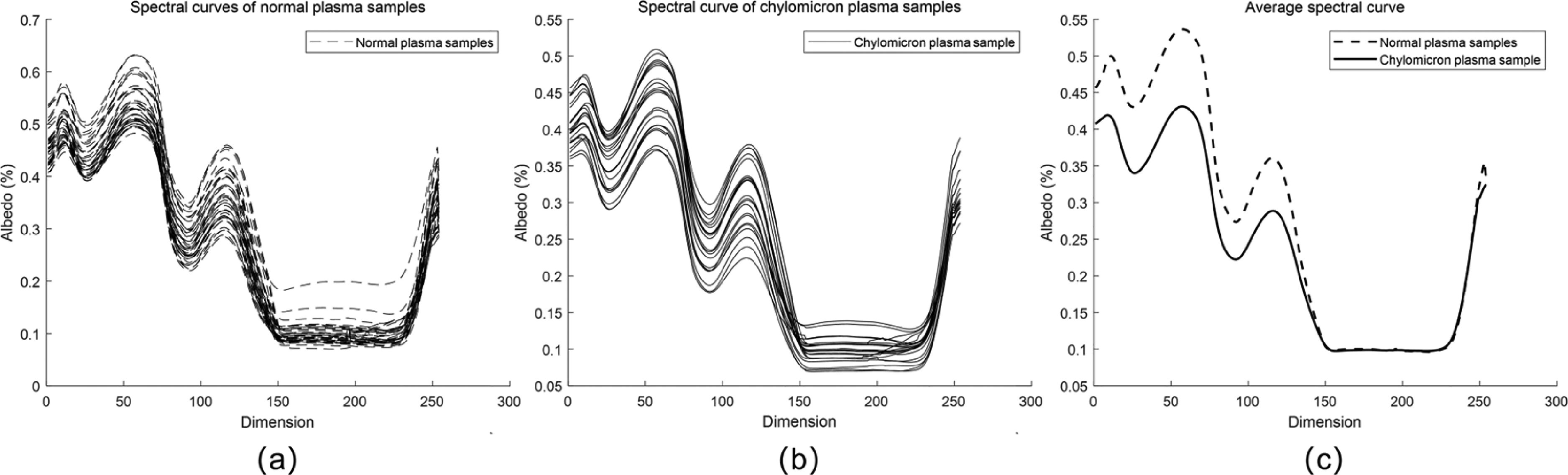
(a) Spectral curves of the normal plasma samples. (b) Spectral curves of the chylous plasma samples. (c) Mean curve of the spectral data between the normal and chylous plasma samples.

The results showed that the variations in trends in the spectral curves of all the plasma samples were roughly similar, and obvious wave peaks could be observed with relatively clear spectral characteristics. The average spectral curves of various samples were obtained, as shown in Figure 1c.

The first 150 characteristic bands showed significant differences between the reflectance of normal and chylous plasma; the reflectance of normal plasma was higher as compared to that of chylous plasma in each band. These results showed that the classification based on plasma spectral reflectance was feasible.

Analysis of the Results of a Plasma Classification Model

Normal and chylous plasma were classified using the first collected data set. Classification effect comparison of different models, set up the same random number in the function, to ensure the consistency between the training set and testing set. In each experiment using different random numbers reduces the happening of the accident.

The effects of each model are presented in Figure 2. The accuracies of the decision tree, GaussianNB, perceptron, and stochastic gradient descent models were 95.83%, 91.67%, 79.17%, and 75%, respectively.

Figure 2.

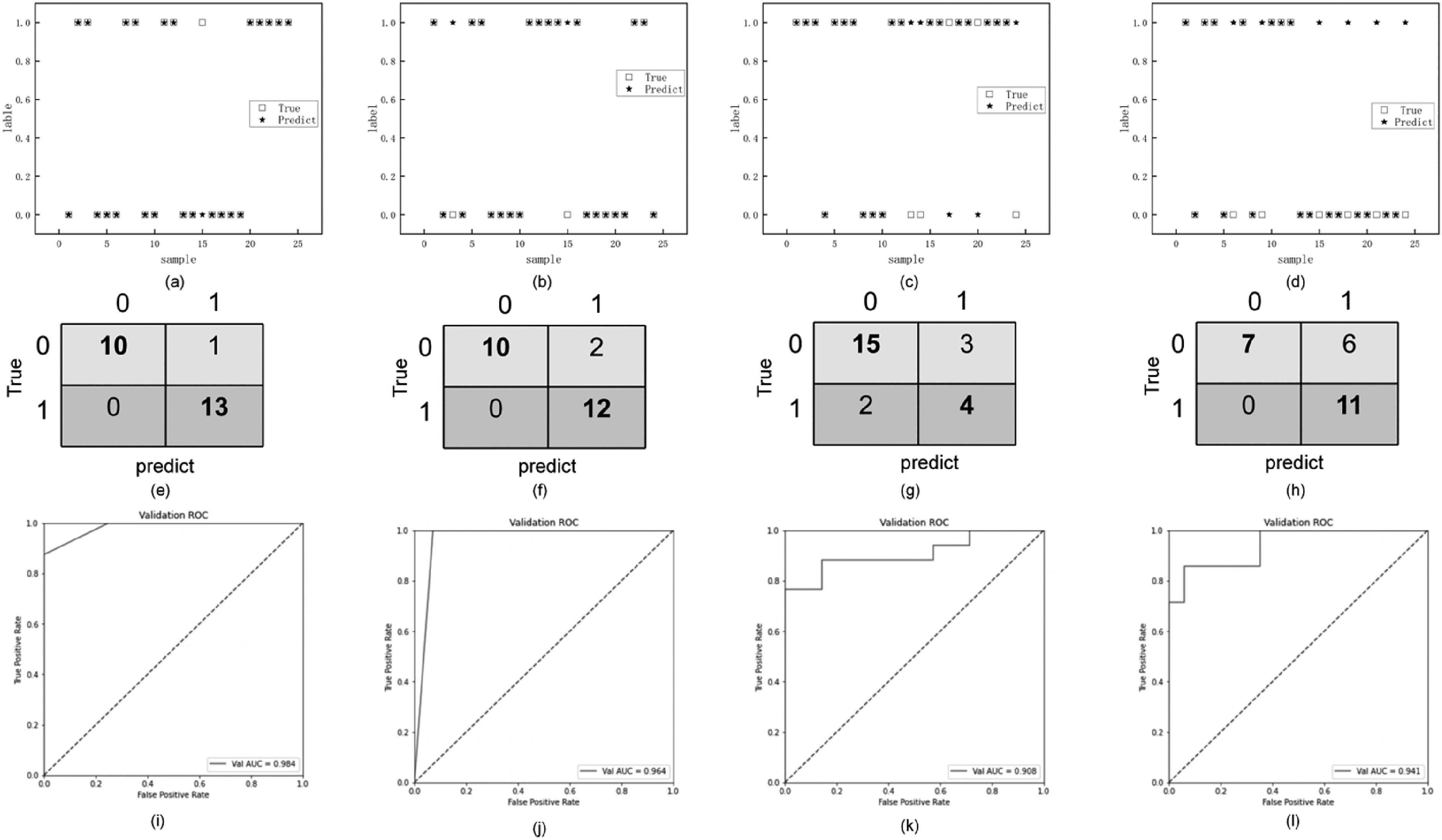
Comparison between the classification results of each model and the real results.

Figures 2a–2d show the comparison between the classification results of each model and the real results. The pink five-pointed star and blue circular patterns represent the predicted and real results. The results showed a successive decrease in the classification effects. The confusion matrix of each model was drawn to compare the classification results of the models more intuitively, as shown in Figures 2e–2h. The results presented by the confusion matrix further confirmed that the classification effects of decision tree, GaussianNB, perceptron, and stochastic gradient descent showed sequentially decreasing results. The ROC curve was drawn based on the confusion matrix to obtain the AUC values and evaluate the prediction ability of the model, as shown in Figures 2i–2l. The AUC value of the decision tree was the highest, which indicates that this model has the best prediction.

In order to reduce the contingency of the training process, five experiments were performed on the model, and the results of each time were compared, as shown in Figure 3a.

Figure 3.

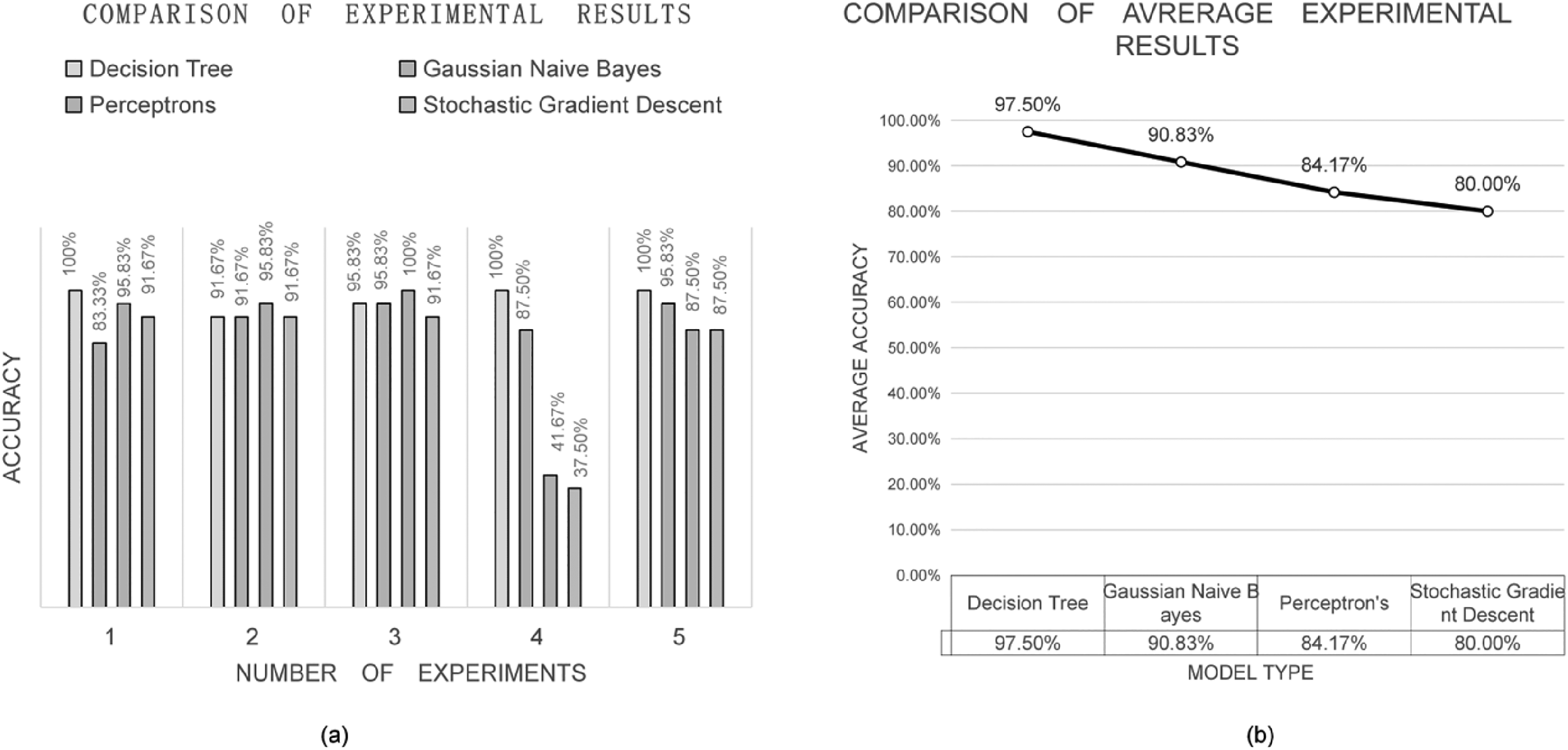
(a) Comparison of the results of five experiments. (b) Comparison of the training results with mean values.

The accuracy of the decision tree was the most stable and high in each experiment. Moreover, the accuracies of other models decreased significantly in the fourth experiment, showing high instability. In order to demonstrate the model effects more comprehensively, the results were compared with the mean values, as shown in Figure 3b.

Among the models, the decision tree exhibited high accuracy, while that of the other three models decreased. The good effect of the decision tree was largely due to its high stability, showing good results in all the experiments.

Analysis of the Effects of Feature Dimension Reduction on the Model

The originally collected data contained 254 bands. The feature dimensions were reduced using the continuous projection method. The results after dimensionality reduction are shown in Figure 4.

Figure 4.

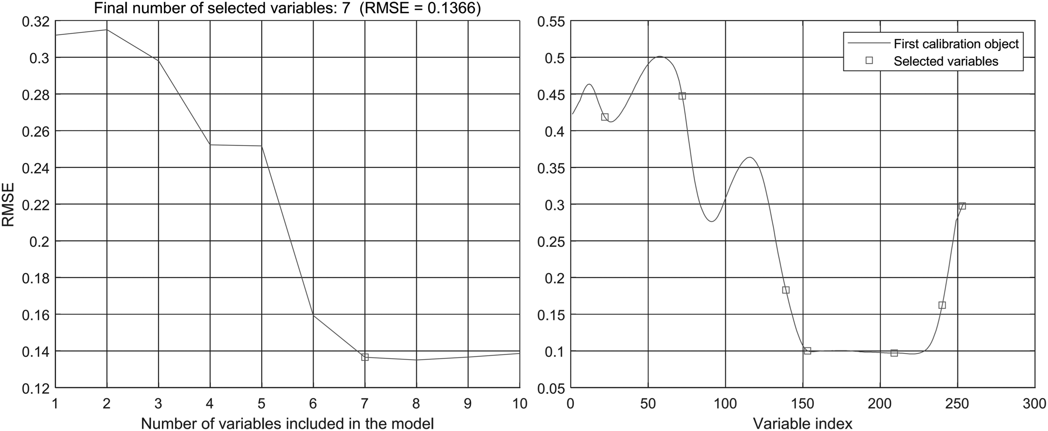
Results of the feature dimension reduction using the continuous projection method.

The RMSE of the model decreased with the increase in the number of bands from 1 to 7. Finally, a total of seven feature bands were selected to replace the 254 bands in the original data. The selected band locations were 22, 72, 139, 153, 209, 240, and 253, corresponding to 962.93, 1122.37, 1338.87, 1380.21, 1558.16, 1656.56, and 1697.8 nm, respectively.

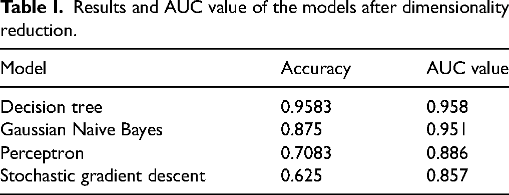
The dimensionality reduction tests were performed, and the effects of each model are listed in Table I. The accuracies of the models decreased in the order of decision tree, GaussianNB, perceptron, and stochastic gradient descent models, and the effects of the models, except the decision tree model, showed a greater decrease as compared to that of the whole band. The AUC value of each model was calculated and compared. The results showed that the AUC value of the decision tree model was the highest, suggesting the best prediction result.

Table I.

Results and AUC value of the models after dimensionality reduction.

Model	Accuracy	AUC value
Decision tree	0.9583	0.958
Gaussian Naive Bayes	0.875	0.951
Perceptron	0.7083	0.886
Stochastic gradient descent	0.625	0.857

Each model underwent five experiments to reduce the contingency of the training process, as shown in Figure 5a.

Figure 5.

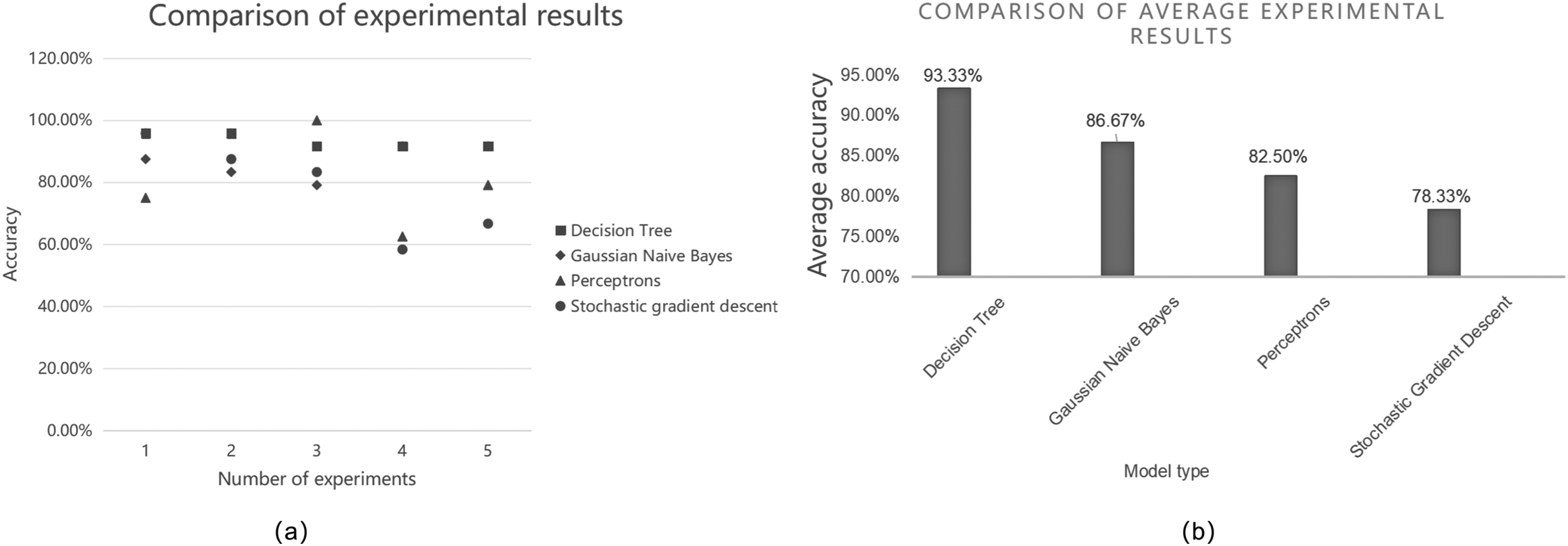
(a) Comparison of the five experiments results after feature dimension reduction. (b) Comparison of training average results after feature dimension reduction.

After dimensionality reduction, the accuracy of the decision tree maintained good stability, while that of GaussianNB showed an overall reduction. Moreover, the accuracies of perceptron and stochastic gradient descent models also showed a significant decrease in accuracy with obvious volatility in the fourth experiment. The averages of these results were taken to present the effectiveness of the model, as shown in Figure 5b.

After dimensionality reduction, the decision tree model still exhibited high average accuracy, while those of the other three models decreased, and the differences between each model and the full band were more obvious. Therefore, the decision tree model could achieve a better classification effect after the dimensionality reduction. After the automatic standardization of data, the average accuracy of the five experiments was compared to eliminate noise interference, as listed in Table II.

Table II.

Comparison of model average accuracies before and after data pre-processing.

Model	No pre-processing		Automatic standardization of pre-processing
Model	Full band	Feature bands	Full band	Feature bands
Decision tree	0.975	0.9333	0.975	0.95
Gaussian Naive Bayes	0.9083	0.8667	0.9083	0.9167
Perceptron	0.8417	0.825	0.80	0.6667
Stochastic gradient descent	0.80	0.7833	0.8417	0.675

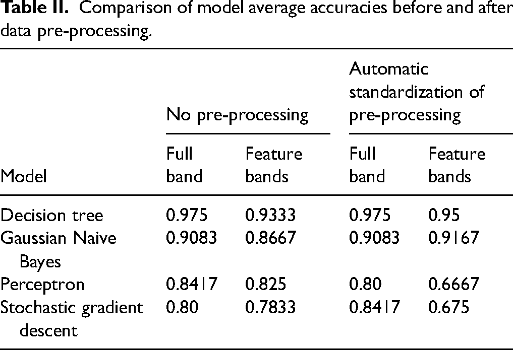
The data comparison showed that the automatic standardized data pre-processing could not greatly improve the accuracy of the full-band test; instead, the accuracy of the perceptron model decreased. In the feature band test, the accuracy of the pre-processed data of the decision tree and GaussianNB models improved.

Classification of Plasma Using CIs

In addition to the classification of plasma as normal and chylous plasma, the degree of chylous was further differentiated. The data set collected for the second time is used for the experiment. Similarly, the same random number is set during the comparison of different model experiments to ensure that the divided training set is consistent with the test set. In order to avoid contingency in each experiment, different random numbers were set for the experiment. Four models, including decision tree, GaussianNB, perceptron, and stochastic gradient descent models, were used in this study. The decision tree model exhibited the best effect with an accuracy of 87.5%, while the accuracies of GaussianNB, perceptron, and stochastic gradient descent models were 50%, 43.75%, and 56.25%, respectively. The results of the decision tree models are presented in Figures 6a and 6b.

Figure 6.

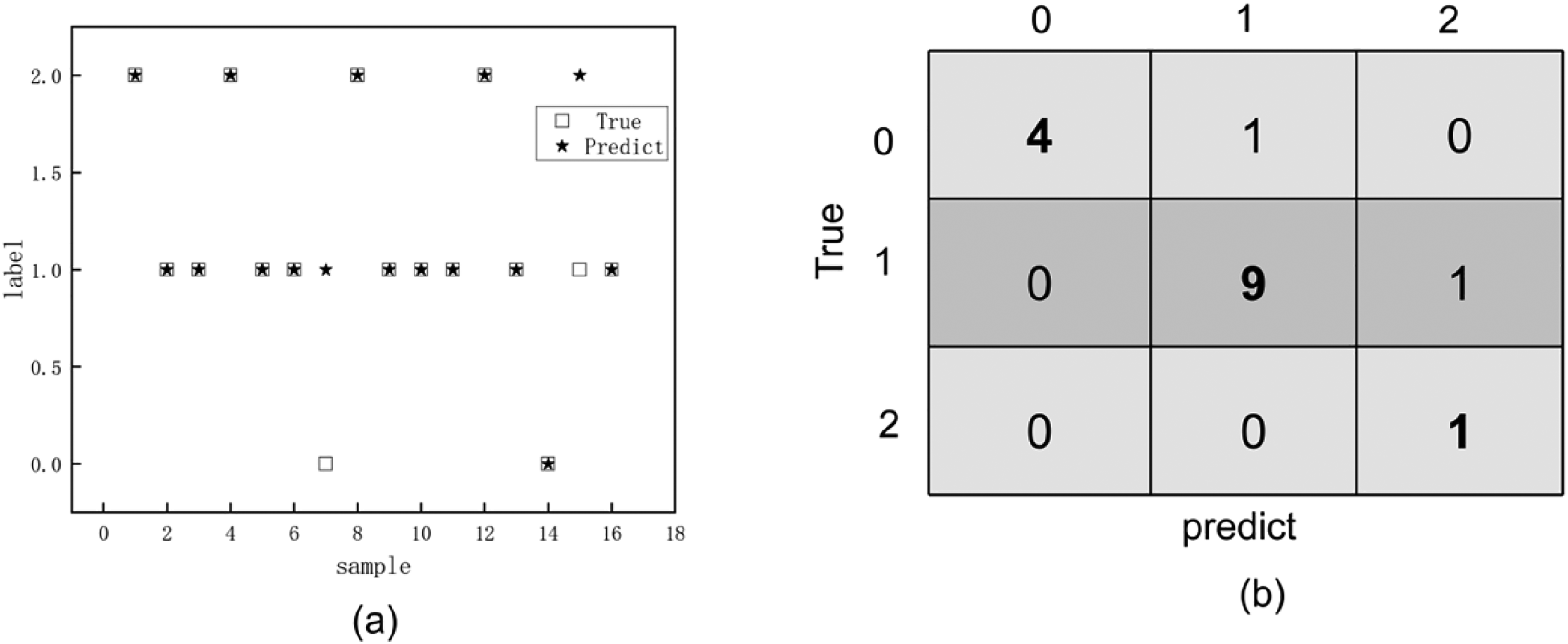
(a) Classification results of decision tree model. (b) Confusion matrix of classification results.

As shown in Figure 6a, the two labels were not correctly classified. The results were further clarified by drawing the confusion matrix of the model, as shown in Figure 6b. The data on the diagonal of the matrix were correctly classified, showing two misclassified samples. The continuous projection method was used for the feature dimension reduction. The results of dimension reduction are shown in Figures 7a and 7b.

Figure 7.

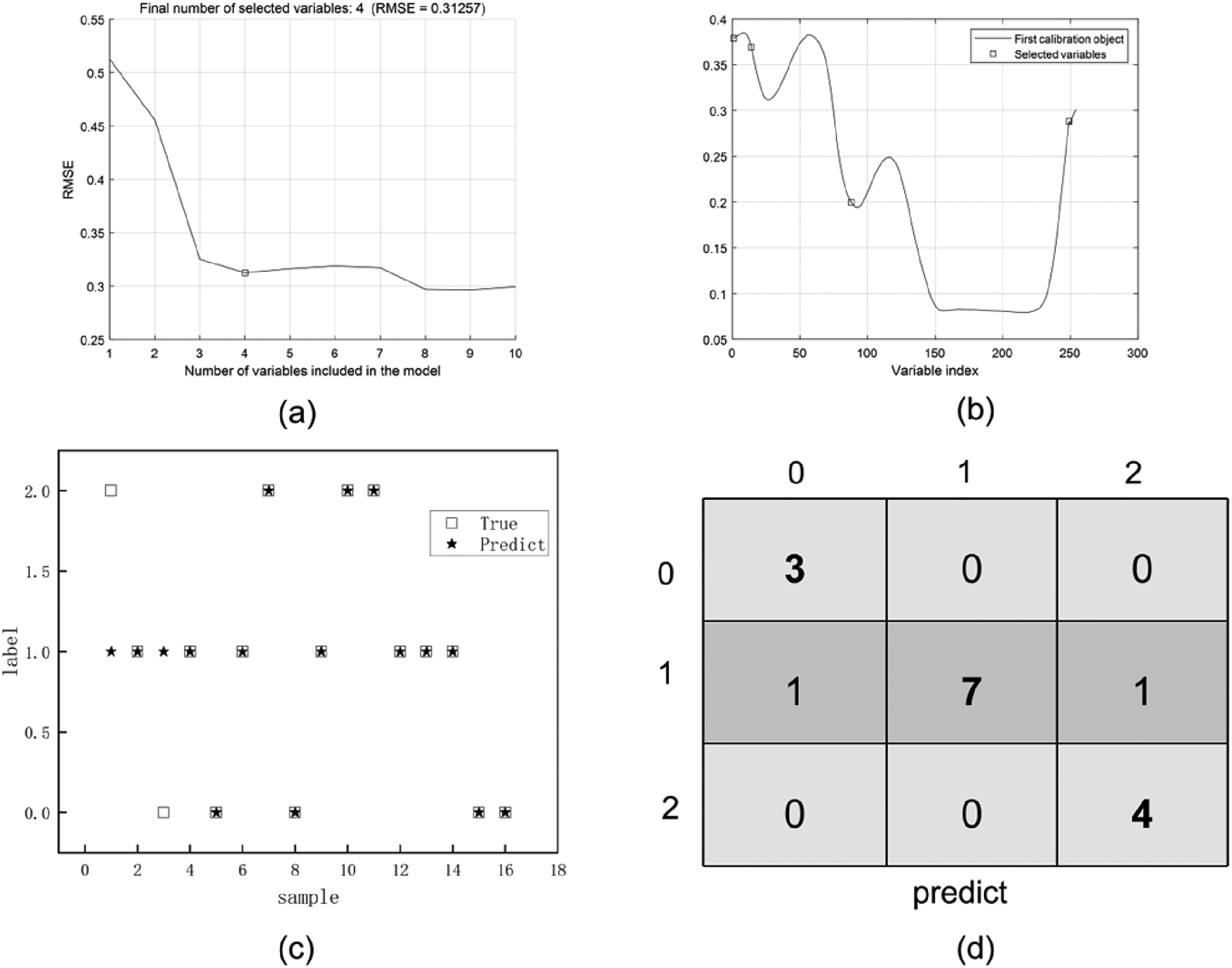
(a, b) Results of feature dimension reduction using the continuous projection method. (c, d) Classification results of the decision tree model after the feature dimension reduction.

The RMSE of the model continuously decreased with the increase in the number of bands from 1 to 4, and finally, four feature bands were selected. The selected band locations were 1, 14, 88, and 249, which corresponded to 895.91, 937.41, 1173.34, and 1685.11 nm, respectively. The test accuracy of the decision tree was 87.5%, showing the best accuracy, as shown in Figures 7c and 7d.

The two misclassified samples, as shown in Figure 7c, further showed that the classification prediction effect was more intuitive. The confusion matrix of the model was drawn, as shown in Figure 7d, demonstrating more careful classification results. The decision process of the decision tree model is presented in Figure S4 (Supplemental Material).

In the whole decision-making process, there were four layers down from the top node with different discriminant conditions. First, the fourth band was analyzed, and the 64 training samples were divided into 39 samples labeled as “1”, and 25 samples labeled as “0” and developed downward based on their respective discriminative conditions.

In order to reduce the contingency of experimental results, five experiments were performed on the model, and the mean values of the results were compared. The decision tree model exhibited the best results, as shown in Figure 8.

Figure 8.

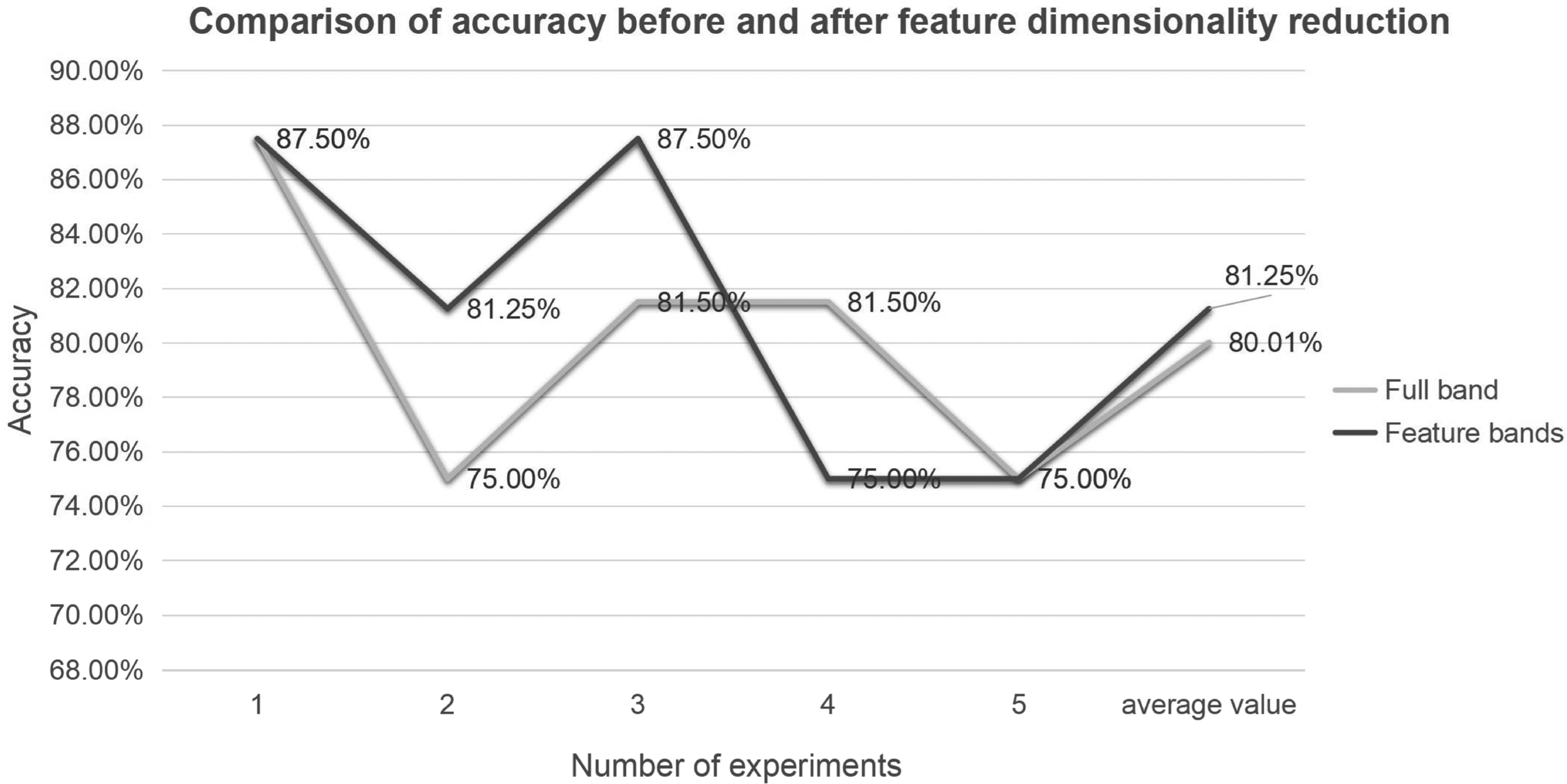
Comparison of accuracy before and after feature dimension reduction.

The results before and after the feature dimensionality reduction were not very stable, showing a certain range of fluctuations. However, the final mean value remained above 80%. The effects of feature dimensionality reduction reached those of the whole band. The performance of the model was evaluated using its recall ratio. The recall ratio of each model before and after feature dimension reduction is listed in Table III.

Table III.

Comparison of the recall of each model before and after the feature dimension reduction.

Model	Full band	Feature bands
Decision tree	0.83	0.81
Gaussian Naive Bayes	0.50	0.61
Perceptron	0.44	0.33
Stochastic gradient descent	0.47	0.33

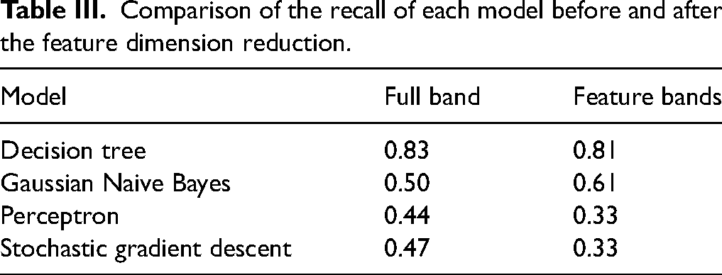
The closer the recall ratio to 1, the better the performance of the model. Only the recall ratio of the decision tree model reached above 0.8 before and after the dimension reduction. Therefore, the decision tree model was identified to have the best performance.

Data Pre-Processing Effect Comparison

In order to eliminate the noise interference, the average accuracy of each model was compared after the automatic standardization of data, as listed in Table IV.

Table IV.

Comparison of the average accuracy of the models, before and after data pre-processing.

Model	No pre-processing occurs		Automatic standardization of pre-processing
Model	Full band	Feature bands	Full band	Feature bands
Decision tree	0.8001	0.8125	0.825	0.8125
Gaussian Naive Bayes	0.525	0.5625	0.625	0.6125
Perceptron	0.3625	0.40	0.4625	0.3875
Stochastic gradient descent	0.475	0.3373	0.4875	0.45

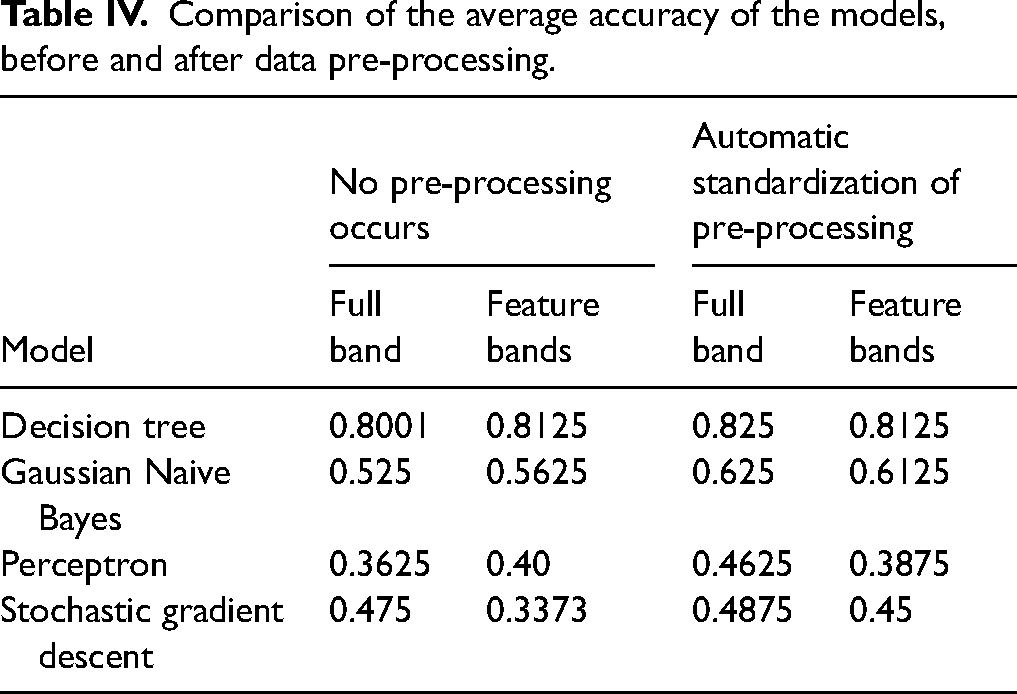
The data comparison showed that the accuracy of each model improved to a certain extent after the automatic standardization of data during the full-band test. In the feature band test, the effects of the decision tree model on the pre-processed data remained the same, while those of GaussianNB and stochastic gradient descent models improved. Moreover, the effects of perceptron decreased.

Conclusion

The results showed that the analysis and testing of the full band data of plasma samples showed that the classification of decision tree and GaussianNB models was better. The average accuracy of the decision tree and GaussianNB models was over 90%, and that of the decision tree model was 97.5%. The feature dimension reduction using the continuous projection method resulted in the selection of seven feature bands for testing. These seven bands included 962.93, 1122.37, 1338.87, 1380.21, 1558.16, 1656.56, and 1697.8 nm. The results of these seven feature bands showed that the accuracy of decision tree classification could reach 93.33%. Therefore, the comparison of the four models showed that the effects of the decision tree model were the most stable, and those of the full-band analysis could be achieved using the seven feature bands. The automatic standardization of data pre-processing improved the accuracy, but it was not obvious.

Four algorithms, including decision tree, GaussianNB, perceptron, and stochastic gradient descent, were used to detect the chylous plasma using different CIs. The best accuracy was that of the decision tree model, which reached 87.5%. After the feature dimension reduction of the data, four feature bands, including 895.91, 937.41, 1173.34, and 1685.11 nm, were selected. After the feature dimension reduction of data, the decision tree model showed the best effects, with an average accuracy of 80.01% and the effects close to the full band.

Chylous plasma could be easily determined based on a few characteristic bands. Furthermore, the chylous plasma with different CIs could also be distinguished, thereby greatly reducing the calculation amount and complexity of detection work, saving detection time, and improving work efficiency. However, the number of samples collected in this study was small, and the data was not rich enough; this might affect the accuracy of these results as well as the generalization ability of the model to a certain extent. In future studies, the data sets should be enriched and expanded to further optimize the model parameters and achieve better results. At the same time, further studies on the chemical interpretation of selected features should be strengthened in future studies, so as to make the relationship between extracted features and chylous plasma detection clearer.

Supplemental Material

sj-docx-1-asp-10.1177_00037028231214802 - Supplemental material for Detection of Chylous Plasma Based on Machine Learning and Hyperspectral Techniques

Supplemental material, sj-docx-1-asp-10.1177_00037028231214802 for Detection of Chylous Plasma Based on Machine Learning and Hyperspectral Techniques by Yafei Liu, Jianxiu Lai, Liying Hu, Meiyan Kang, Siqi Wei, Suyun Lian and Haijun Huang, Hao Cheng, Mengshan Li, Lixin Guan in Applied Spectroscopy

Footnotes

Data Availability Statement

The data sets generated during or analyzed during the current study are available from the corresponding author upon reasonable request.

Declaration of Conflicting Interests

The authors declared no potential conflicts of interest with respect to the research, authorship, and/or publication of this article.

Funding

The authors disclosed receipt of the following financial support for the research, authorship, and/or publication of this article: This work was supported by the National Natural Science Foundation of China (grant numbers 51663001, 52063002, and 42061067).

ORCID iD

Yafei Liu

Supplemental Material

All supplemental material mentioned in the text is available in the online version of the journal.

References

Sukkriang

Chanprasertpinyo

Wattanapisit

Punsawad

, et al. “Correlation of Body Visceral Fat Rating with Serum Lipid Profile and Fasting Blood Sugar in Obese Adults Using a Noninvasive Machine”. Heliyon. 2021. 7(2): e06264. https://doi.org/10.1016/j.heliyon.2021.e06264

Randolph

G.J.

Miller

N.E.

. “Lymphatic Transport of High-Density Lipoproteins and Chylomicrons”. J. Clin. Invest. 2014. 124(3): 929–935. https://doi.org/10.1172/JCI71610

Baass

Paquette

Bernard

Hegle

R.A.

. “Familial Chylomicronemia Syndrome: An Under-Recognized Cause of Severe Hypertriglyceridaemia”. J. Intern. Med. 2020. 287(4): 340–348. https://doi.org/10.1111/joim.13016

Michael Strong

Katz

. “Blood-Bank Testing for Infectious Diseases: How Safe is Blood Transfusion?” Trends Mol. Med. 2002. 8(7): 355–358. https://doi.org/10.1016/s1471-4914(02)02361-4

Hirata

Inokuchi

Tsuneya

Hoshioka

, et al. “A Case of Fatal Fulminant Fat Embolism Syndrome Following Multiple Fractures Resulting from a Fall”. J Forensic Sci. 2022. 67(5): 2115–2121. https://doi.org/10.1111/1556-4029.15083

Huang

Jiang

, et al. “A Multi-Step Approach for Tongue Image Classification in Patients with Diabetes”. Comput. Biol. Med. 2022. 149: 105935. https://doi.org/10.1016/j.compbiomed.2022.105935. ISSN:0010-4825.

Xie

Huang

Liu

, et al. “Quality Analysis of Physicochemical Parameters of Chylous Plasma”. J. Lab. Clin. Med. 2020. 17(23): 3482–3486.

Tian

Xie

Duan

Chen

, et al. Method and System for Detection of Plasma Chylous Degree. CN111829962A. Filed 2022. Issued 2023.

Chu

Zhang

, et al. “Study on Nondestructive Detecting Gannan Navel Pesticide Residue with Hyperspectral Imaging Technology”. Spectrosc. Spectral. Anal. [Guangpuxue Yu Guangpu Fenxi]. 2016. 36(12): 4034–4042.

10.

Zhang

, et al. “Progress Study on the Application of Hyperspectral Imaging Technology in the Pharmaceutical Field”. J. Pharm. Anal. 2021. 41(08): 1360–1367.

11.

Liu

Lyu

Hou

Gao

, et al. “A Novel Spectral Matching Approach for Pigment: Spectral Subsection Identification Considering Ion Absorption Characteristics”. Remote Sens. 2020. 12(20): 3415. https://doi.org/10.3390/rs12203415

12.

Zhang

Ding

Lin

Wang

, et al. “Transmission Versus Reflection Spectroscopy for Discrimination of Human and Nonhuman Blood”. Infrared Phys. Technol. 2019. 99: 1–4. https://doi.org/10.1016/j.infrared.2019.03.035. ISSN:1350-4495.

13.

Feng

Ding

Cui

. “Detection of Blood Spots in Eggs by Hyperspectral Transmittance Imaging”. Int. J. Agric. Biol. Eng. 2019. 12(6): 209–223. https://doi.org/10.25165/j.ijabe.20191206.5376

14.

Zhang

Yang

Song

Wang

. “In-Situ Calibration of Relative Reflectance for Visible/Near-Infrared Imaging Spectrometer”. Sens. Lett. 2012. 10(1): 198–204. https://doi.org/10.1166/sl.2012.1845

15.

Dong

Tang

Z.-S.

Hua

Cai

X.-C.

, et al. “Research on Classification Method of Main Poisonous Plants in Alpine Meadow Based on Spectral Characteristic Variables”. Spectrosc. Spectral. Anal. [Guangpuxue Yu Guangpu Fenxi]. 2022. 42(4): 1076–1082. https://doi.org/10.3964/j.issn.1000-0593(2022)04-1076-07

16.

Chen

Shi

Gong

Sun

, et al. “True-Color Three-Dimensional Imaging and Target Classification Based on Hyperspectral Lidar”. Remote Sens. 2019. 11(13): 1541. https://doi.org/10.3390/rs11131541

17.

Wen

Cheng

, et al. “A Model for Genuineness Detection in Genetically and Phenotypically Similar Maize Variety Seeds Based on Hyperspectral Imaging and Machine Learning”. Plant Methods. 2022. 18(1): 81. https://doi.org/10.1186/s13007-022-00918-7

18.

Jia

Liao

, et al. “3-D Gabor Convolutional Neural Network for Hyperspectral Image Classification”. IEEE Trans. Geosci. Remote Sens. 2022. 60: 1–6. https://doi.org/10.1109/TGRS.2021.3087186. ISSN:0196-2892.

19.

Chen

Bai

Zhang

Zhu

Zhang

. “Hyperspectral Detection of Sugar Content for Sugar-Sweetened Apples Based on Sample Grouping and SPA Feature Selecting Methods”. Infrared Phys. Technol. 2022. 125: 104240. https://doi.org/10.1016/j.infrared.2022.104240. ISSN:1350-4495.

20.

Kayet

Pathak

Singh

C.P.

Chowdary

V.M.

, et al. “Vegetation Health Conditions Assessment and Mapping Using AVIRIS-NG Hyperspectral and Field Spectroscopy Data for Environmental Impact Assessment in Coal Mining Sites”. Ecotoxicol. Environ. Saf. 2022. 239: 113650. https://doi.org/10.1016/j.ecoenv.2022.113650. ISSN:0147-6513.

21.

Zhang

Bai

Huang

, et al. “Detection of Rice Spikelet Flowering for Hybrid Rice Seed Production Using Hyperspectral Technique and Machine Learning”. Agriculture. 2022. 12(6): 755. https://doi.org/10.3390/agriculture12060755

Supplementary Material

Please find the following supplemental material available below.

For Open Access articles published under a Creative Commons License, all supplemental material carries the same license as the article it is associated with.

For non-Open Access articles published, all supplemental material carries a non-exclusive license, and permission requests for re-use of supplemental material or any part of supplemental material shall be sent directly to the copyright owner as specified in the copyright notice associated with the article.

0.00 MB

4.64 MB