Analysis of Lithium Aging Using Machine Learning-Enhanced Spectroscopy Techniques

Abstract

Lithium compounds such as lithium hydride (LiH) and lithium hydroxide (LiOH) have a wide range of industrial applications, but are highly reactive in environments with H₂O and CO₂. These reactions lead to the ingrowth of secondary lithium compounds, which can alter the homogeneity and affect the application of particular lithium chemicals. This study performed an exploratory analysis of different lithium compounds using laser-induced breakdown spectroscopy (LIBS) and Raman spectroscopy. Machine learning models are trained on the recorded spectral data to discriminate emission features that differ between LiH, LiOH, and Li₂CO₃ to perform high-fidelity classification. Support vector machine classifiers yield perfect prediction accuracy between the three compounds with optimal training time. Multivariate methods are then used to produce regression models quantifying the ingrowth of LiOH in LiH. Performing a mid-level data fusion of selected LIBS and Raman features with partial least-squares regression produces the superlative model with a root mean square error of 2.5 wt $%$ and a detection limit of 6.3 wt $%$ .

Keywords

Laser-induced breakdown spectroscopy LIBS‌Raman spectroscopy machine learning data fusion lithium lithium aging

Introduction

Lithium compounds are critical to several major industries, including the production of commercial batteries¹ and a variety of pharmaceuticals.² Lithium also plays an important role in radiation science and in the nuclear fuel cycle. Lithium compounds enable the production of lightweight materials for neutron shielding, specifically to capture thermal neutrons without emitting a capture gamma.^3,4 Lithium salts are key components of the breeding blanket in next-generation nuclear power reactors; the formation of tritium from lithium enables deuterium–tritium fusion reactions.^5–8 The quality and homogeneity of lithium compounds must be ensured via chemical analysis; the ingrowth of secondary lithium compounds can change fundamental reaction cross sections of the material, ultimately affecting its performance for a given application.⁹ The compounds lithium hydride (LiH), lithium hydroxide (LiOH), and Li₂CO₃ are of particular interest to this ingrowth and characterization problem. The formation of LiOH is described by chemical Eq. 1, while the formation of Li₂CO₃ is governed by chemical Eqs. 2 to 4.^10,11

LiH + H_{2} O ⟶ LiOH + H_{2}

(1)

LiOH + LiH ⟶ {Li}_{2} O + H_{2}

(2)

2 LiOH + H_{2} O ⇌ 2 LiOH \cdot H_{2} O

(3)

2 LiOH \cdot H_{2} O + {CO}_{2} ⟶ {Li}_{2} {CO}_{3} + 3 H_{2} O .

(4)

Implementing a high-fidelity chemical analysis technique to study and quantify the growth of these compounds in lithium samples is the first step needed to optimize storage conditions to mitigate environmental aging. Laser-induced breakdown spectroscopy (LIBS) and Raman spectroscopy are two commonly used techniques to analyze material chemistry from recorded spectral emissions which have been implemented in lithium analysis studies.^12–18 Wood et al.¹⁹ implemented LIBS with multivariate statistics to quantify isotopic concentrations in LiOH. Pinson et al.²⁰ used a tandem LIBS–Raman setup to perform low-level data fusion of spectra from aged LiH samples to optimize environmental storage conditions.

Laser-induced breakdown spectroscopy (LIBS) and Raman have previously been used in tandem for analytical chemistry applications such as the identification of minerals and organics in geological samples,^21,22 space exploration,^23,24 and the analysis of archaeological artifacts.²⁵ Recent studies have used both techniques with machine learning (ML) models and data fusion methodologies to perform high-fidelity classification and regression analyses of geochemical samples^26–30 and hydrocarbon fuels.³¹ A wide variety of ML models have been implemented for the analysis of complex actinide spectra from nuclear debris and plutonium alloys, yielding markedly improved results in diagnostic analysis of nuclear material.³² These advances in analytical techniques and the results of these investigations prove the utility of data science techniques in discriminating feature changes across complex spectral data sets. This paper explores the capabilities of ML models to learn differences between several lithium compounds based on spectral emission features and to produce high-fidelity models that relate spectral differences to the chemical properties of a set of lithium samples.

We present the analysis of lithium compounds using spectra recorded from a tandem LIBS–Raman experimental setup. We analyzed recorded spectra of pure LiH, LiOH, and Li₂CO₃, along with three different mixed LiH–LiOH samples (90/10, 75/25, and 50/50 wt% LiH/LiOH). We implement ensemble methods, support vector machines (SVMs), neural networks, and $k$ -nearest neighbor methods trained on the LIBS data and perform a classification analysis of the three different compounds. LIBS and Raman spectra are used with a mid-level data fusion scheme to construct multivariate regression models quantifying LiOH ingrowth in the LiH samples. The regression error and sensitivity of the fused model are compared to that of multivariate regressions constructed with LIBS and Raman data alone to understand how fusing spectral features improves prediction fidelity.

Experimental

Sample Preparation

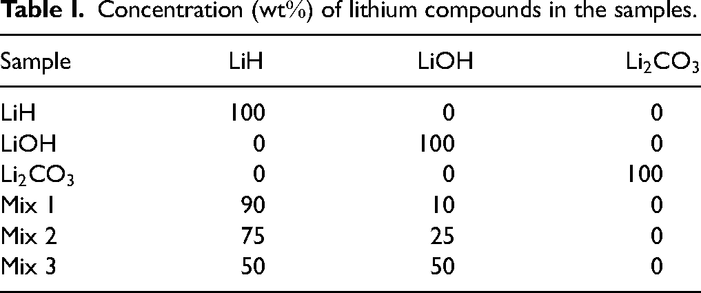
Powder samples of LiH (Sigma Aldrich, 95% pure), LiOH (Sigma Aldrich, 98% pure), and Li₂CO₃ (Sigma Aldrich, 99% pure) were pressed into pellets inside a dry nitrogen glove box. Previous work by Sifuentes et al.¹² showed that a relative humidity of 1% has led to a very low mass increase in LiH samples. Liquid nitrogen boil-off was used to purge a glove box and successfully kept the humidity conditions at or near this level (ranging from 1.1% to 1.7%) as measured with a humidity probe. Table I outlines the sample composition matrix with all values having units of weight percent mass. The relative uncertainty is <1% for all concentration values in the table with the dominant form of error resulting from the accuracy of the scale. The powders for the mixed samples were ground with a mortar and pestle to ensure uniform particle size, weighed, then combined in a Fluxana MUK mixer, shaken to achieve homogeneity, and then pressed using a Specac Ltd. minipress at 1.5 tons for 3 min. The sample matrix was structured to mimic the degradation process of LiOH ingrowth into LiH by pairing each set of analytes together at multiple concentrations.

Table I.

Concentration (wt $%$ ) of lithium compounds in the samples.

Sample	LiH	LiOH	Li₂CO₃
LiH	100	0	0
LiOH	0	100	0
Li₂CO₃	0	0	100
Mix 1	90	10	0
Mix 2	75	25	0
Mix 3	50	50	0

Once pressurized, the samples were placed in a conflat flange sample cell with a top viewport, as shown in Figure 1, to maintain the dry environment while transferring the sample to the laser table and throughout the analysis. The viewport allowed for laser interaction with the sample as well as atomic emission collection. Samples were affixed to the bottom of the conflat flange cell using a thin layer of vacuum grease. The grease served to keep the samples from shifting while maneuvering the equipment and during the ablation process. The sample cells were thoroughly disassembled and cleaned between sample set tests to prevent cross-contamination. It should be noted that although LIBS experiments often use vacuum, argon, or helium as buffer gases to enhance the signal, this work used nitrogen to simulate the most common environments for LiH handling and storage.

Figure 1.

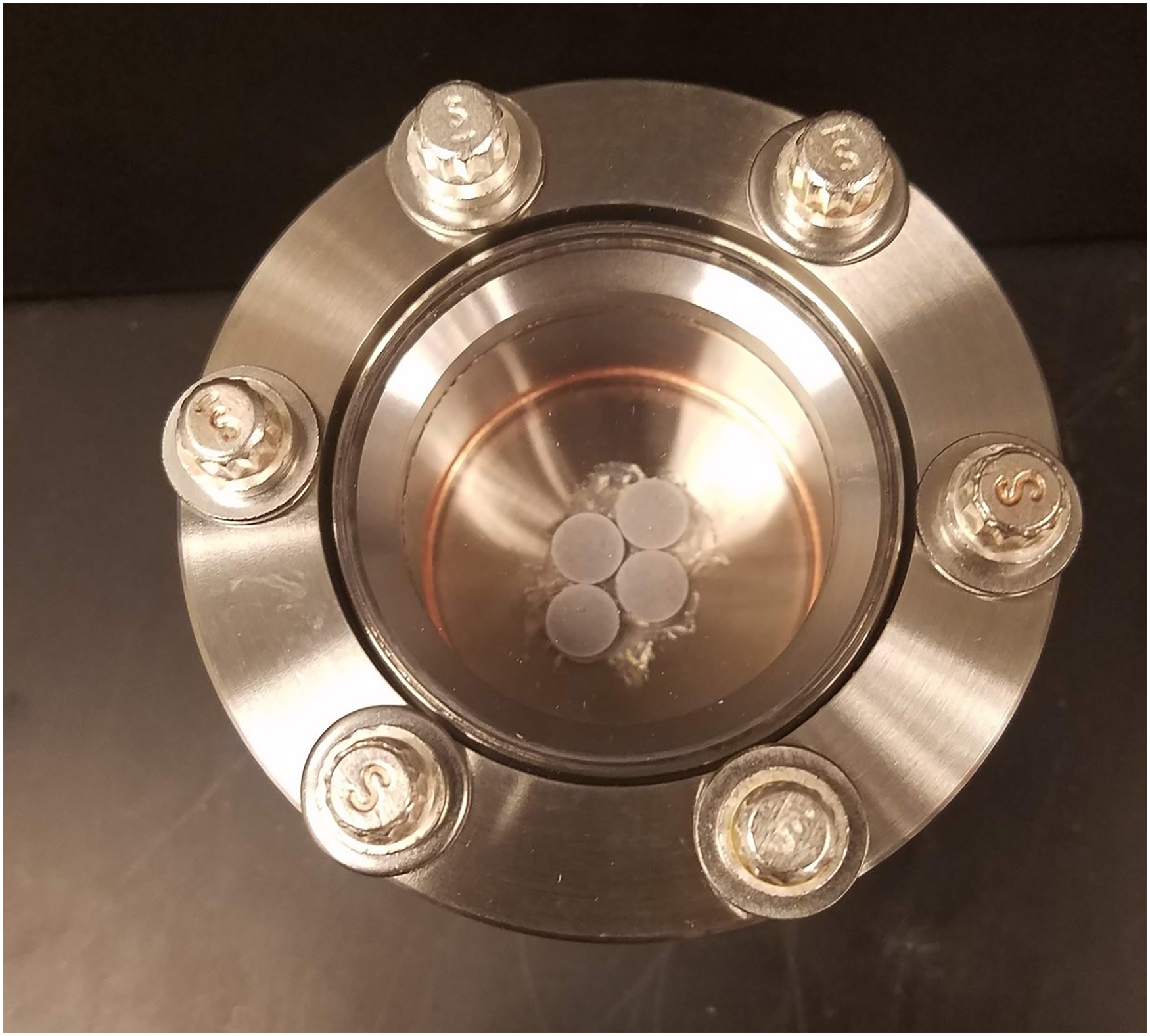
Conflat flange sample cell with 3.2 mm thick ultraviolet fused silica viewport; samples are 2.5 cm from the outside face of the viewport.

Spectroscopic Setup and Measurements

A dual Raman–LIBS experimental setup illustrated in Figure 2 was implemented in this study. The use of a single setup to conduct both Raman and LIBS has the obvious advantage of reducing the experimental time, maintaining the sample condition, and streamlining the analytical process. Shameem et al.³³ demonstrated the versatility of the echelle spectrograph for use in both LIBS and Raman spectroscopy using a single set-up. The only parameter changed between LIBS and Raman measurements is energy fluence. This is accomplished by using a defocusing lens and reducing the laser power during Raman measurements to prevent ablation.

Figure 2.

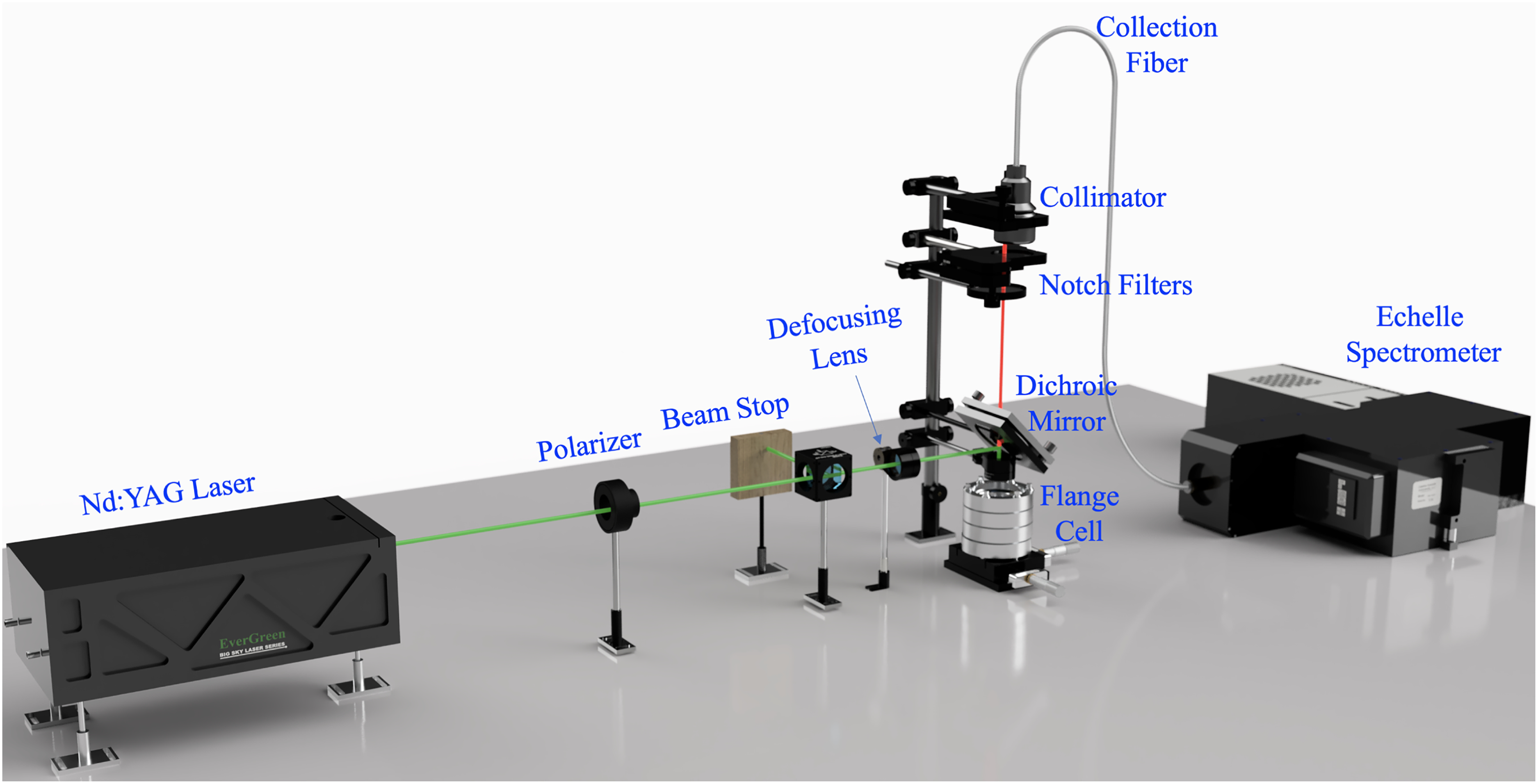
Tandem LIBS–Raman setup used for sample analysis.

This study employed a 10 Hz Q-switched neodymium-doped yttrium aluminum garnet laser (Quantel Evergreen) operating at 532 nm with a 10 ns pulse width. A digital delay generator (Berkeley Nucleonics 577) was used as a trigger source for both the laser and the intensified charge-coupled device (iCCD) camera. For Raman measurements, the light is directed through a defocusing lens set twice the focal length ( $f = + 75 mm$ ) from the 550 nm high-pass dichroic mirror to avoid focusing the laser onto the mirror and ablating the surface. The laser is then directed through the final focusing lens ( $f = + 100 mm$ ) and onto the sample through the viewport on the conflat flange cell. The Raman scattered light incident upon the final focusing lens is then collimated back along the path of the laser pulse. Light transmitted through the dichroic mirror then passes through two notch filters (OD-4 and OD-6) and into the light collection optics for the optical fiber. For LIBS measurements, the defocusing lens is simply rotated out of the way and the laser power is increased to induce ablation.

An Echelle spectrograph (Catalina Scientific EMU-120/65) was used to record broadband spectra from 325 to 925 nm with $Δ λ = 0.01$ nm and resolving power $R = 15 000$ . A 25 mm aperture stop was used along with a $30 \times 120 μ$ m slit. The spectrograph was paired with an iCCD camera (Andor USB iStar) to record the dispersed atomic emissions. The broad bandwidth is especially useful in chemometrics with LIBS data because at least some spectral lines from nearly every element are present in this range, making it possible to collect data from every element of interest in a single spectrum. The same benefit is true for conducting Raman spectroscopy. In this study, the laser wavelength was 532 nm, placing a shift of 3600 cm⁻¹ around 658 nm, which was well within the dynamic range of the spectrograph.

Raman measurements were taken prior to LIBS measurements, because of the non-destructive nature of the former. Due to the spot size of the laser at the sample and the field of view of the light collection optics, spectra were taken from five positions on each of the samples. The Raman spectra were acquired by integrating recordings in a single exposure and then accumulating multiple recordings to form the final image. This was done at a repetition rate of 10 Hz for 600 pulses per exposure, repeated for five exposures per sample with a 1 ms exposure time. The iCCD camera gate delay was set at 140 ns with a gate width of 40 ns. The microchannel plate gain was set to a moderate value of 2500 on a 0–4000 nonlinear scale. For LIBS measurements, an unperturbed position was chosen for the beginning of each set of shots. Each set of shots consisted of 20 ablations in a single position. Each sample was ablated in 10 separate positions for a total of 200 spectra per sample. The camera was adjusted to have a gate delay of 1.5 $μ$ s and a gate width of 6.0 $μ$ s to optimize the quality of the recorded signal of the atomic emission spectra.

Analytical Methods

Data Preprocessing and Feature Selection

The raw classification data set consisted of 600 LIBS spectra (200 of each compound), each with 60,001 features. The raw regression data set consisted of 20 LIBS and 20 Raman spectra each of pure LiOH, as well as the Mix 1–3 samples. Each LIBS spectrum had 60 001 features, while each Raman spectrum had 60 295 features. The sheer size of the feature space in this problem underscores the need to follow the ML workflow and implement basic feature selection.

First, the raw spectra in both the classification and regression data sets were normalized using the standard normal variate (SNV) method in Eq. 5: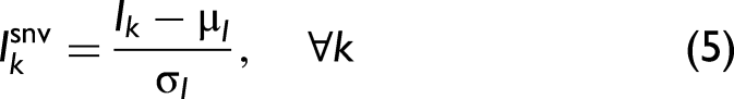

I_{k}^{snv} = \frac{I_{k} - μ_{I}}{σ_{I}}, \forall k

(5)

each spectrum (

I_{k}

) is centered on its mean value (

μ_{I}

) and then divided by the original spectrum standard deviation (

σ_{I}

) to yield the SNV normalized spectrum (

I_{k}^{snv}

). Normalization is commonly implemented in spectroscopic analysis to reduce signal fluctuation in the raw spectra and yield enhanced analytical performance;³⁴ SNV normalization is often implemented in pre-processing LIBS, near-infrared, and Raman spectra for this purpose.^35–37

Feature selection was then implemented on the classification data set by performing a principal component analysis (PCA) on the normalized data and examining the values of the loadings of the wavelengths of the first principal component (PC). This method has been implemented in prior studies to determine which emission wavelengths contribute the most variance in the data set. The wavelength region between 575 and 690 nm was found to have the highest loading values of the first PC, indicating that the features that contribute the most to the differences in the spectral data sets manifest in this region. Figure 3a shows the averaged spectra of each of the three compounds in the classification data set. The feature comparison indicates noticeable differences in the Li I atomic emissions at 610 and 671 nm, as well as the lack of H_α at 656 nm in the Li₂CO₃ spectra. The presence of the Na D₁/D₂ emissions at 589/590 nm stems from minor impurities in the powders used to create the samples. Cutting the LIBS classification data set to this wavelength range reduced the feature size from 60 001 to 23 001.

Figure 3.

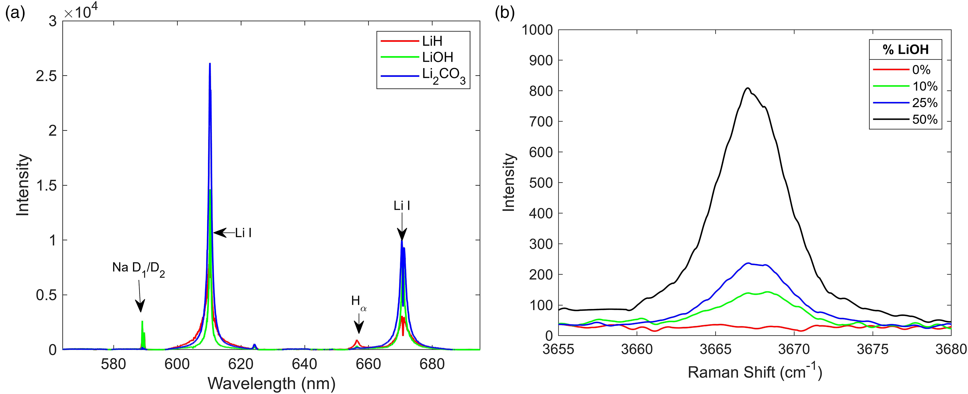
(a) Laser-induced breakdown spectroscopy (LIBS) emission differences between pure LiH, LiOH, and Li₂CO₃ and (b) Raman LiOH $\cdot$ H₂O peak intensity variation versus LiOH concentration.

The same feature selection process was applied to the regression data set; the LIBS regression data features varied most between 595 and 680 nm in the LiH/LiOH mixed sample set. This also follows from Figure 3(a), as most of the variance between these two compounds comes from Li I emissions and H_α at 656 nm. This reduced the size of the LIBS feature space from 60 001 to 17 001. The Raman data set had one major peak at 3667 cm⁻¹ with a high PC loading value, shown in Figure 3b. This peak is attributed to the intermediary compound LiOH $\cdot$ H₂O. Pinson et al.²⁰ also identified this Raman peak and its prominence in lithium samples exposed to humidity for a longer time, which explains its significance in this data set. The recorded Raman spectra of the LiH and LiOH mixture samples were cut to the range between 3655 and 3680 cm⁻¹, reducing the number of Raman features to 442.

Machine Learning Methods and Optimization

Support Vector Machine (SVM)

SVMs classify samples in an $N$ -dimensional (where $N$ is the number of features) space by creating a hyperplane that divides each class of data. An illustration of this method is given in Figure S1 (Supplemental Material). The hyperplanes follow the equation $w^{T} x - b = 0$ , and maximize the distance between points $x_{i}$ and the dividing hyperplane of each class by tuning the margin parameter $b / ‖ w ‖$ . As a result, SVMs tend to perform better in classifying complex data. While SVMs are technically binary classifiers, they can be aggregated into a type of ensemble called an error-correcting output code, which reframes a multiclass problem as several binary classification problems that can each be solved by a different SVM model.³⁸

Ensemble Methods

Tree-based ensemble methods are ML constructs based on decision trees, a supervised learning technique that relates input variables to an output by following branches at decision nodes based on the input attribute values. Tree-based ensembles use groups of decision trees together to achieve better predictive performance by reducing variance and increasing bias. The most common ensemble techniques are bootstrap-aggregating (bagging) and boosting; these are graphically depicted in Figure S2 (Supplemental Material). Bagging uses random replacement sampling to create subsets (S) of the data and independently trains the individual classifier (M), while boosting introduces an adaptive algorithm that focuses on areas in the data set that generates higher misclassifications and trains each model sequentially.^39,40 Whereas bagged models run in parallel and the final prediction is made from an aggregate of each trained model, boosting changes in the input weights for each model depending on the error of the previous iteration to improve the accuracy of subsequent learners.

Artificial Neural Network (ANN)

A neural network takes a series of input variables and multiplies them by weights. Predictors enter an ANN through an input layer and are fed forward to subsequent layers. Each hidden layer contains neurons (nodes), wherein each neuron sums weighted inputs from the previous layer and generates an output by applying an activation function. The output layer sums weighted inputs from the last hidden layer and generates a numerical output via an activation function.^39,41 This process is modeled as a mathematical analog of synaptic communication in biological neural pathways; Figure S3 (Supplemental Material) illustrates a single hidden layer ANN architecture.

K-Nearest Neighbors (KNNs)

K-nearest neighbors (KNN) is a non-parametric technique that predicts the class of an unknown sample based on its proximity to other known samples in the feature space of the data set.⁴² This is illustrated in Figure S4 (Supplemental Material); the number of nearest neighbors $(k)$ and the distance metric used to calculate proximity can be optimized for improved classification performance. In this simple example, the three nearest neighbors to the new prediction point are identified; since two of the three are blue, the prediction would also be in the blue class.

Hyperparameter Optimization

Hyperparameter optimization is a key part of the ML workflow needed to produce models that can make accurate predictions from complex input data without overfitting during training. An automated hyperparameter optimization routine was implemented on all selected classification models discussed above, using a Bayesian optimizer to run through different values of all tunable hyperparameters of each model and changing the values from one iteration to the next to minimize the model error (mean square error). Bayesian optimizers are commonly used in hyperparameter tuning and ML model design to achieve the hyperparameter configuration with the lowest feasible model error.^43,44 The entire LIBS classification data set (800 samples and 2001 features) was split into an 80/20 $%$ training and test split; the hyperparameter tuning was performed on the training split. Each optimization was run for 30 iterations, over which the models were able to converge to a low error value after hyperparameter tuning. Table II shows a comprehensive list of all regression models, tunable hyperparameters, ranges of values examined, and final tuned values of each model. Classification accuracy was evaluated on the tuned models using the remaining test data split. Rao et al.⁴⁵ provides a thorough overview of many of these models and the definitions of their hyperparameters. Furthermore, all computational work in this study was performed in Matlab with functions in the Statistics and ML Toolbox using an Intel i9 CPU; documentation for these learning methods is publicly available, along with detailed descriptions of the hyperparameters for each model.⁴⁶

Table II.

Hyperparameter optimization options and final tuned values for all implemented models.

Model	Hyperparameters	Range	Tuned value
Ensemble	Min. leaf size	1–144	2
	Max. num. splits	1–4000	8
	Num. learning cycles	10–500	32
	Learning method	Bag; AdaBoostM2; RUSBoost	RUSBoost
SVM	Kernel function	Linear; Gaussian; polynomial	Linear
	Kernel scale	0.001–1000	1
	Box constraint	0.001–1000	0.033
KNN	Distance metric	Cosine; Euclidian; Minkowski; Mahalanobis	Cosine
	k	1–600	298
	Distance weight	Equal; inverse; squared inverse	inverse
ANN	Layer size	Narrow; medium; wide; bilayer; trilayer	bilayer
	Number of neurons	2–300	[7; 256]
	Activation function	ReLU; Sigmoid, tanh	ReLU
	Iteration limit	$1 \times 10^{2}$ – $1 \times 10^{4}$	1000
	Regularization ( $λ$ )	$4.99 \times 10^{- 10}$ –0.499	$1.22 \times 10^{- 2}$

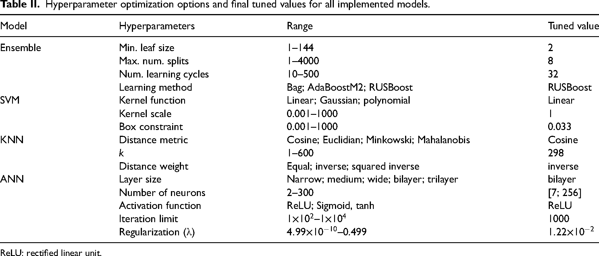
ReLU: rectified linear unit.

Multivariate Regression and Data Fusion

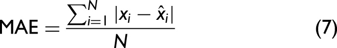
The regression data set, composed of LIBS and Raman spectra of the LiH/LiOH mixes, was used to construct predictive regression models relating changes in spectral feature intensity to the LiOH content of a sample. Principal component regression (PCR) and partial least-squares regression (PLSR) were used; these multivariate regression techniques are very common in a range of quantitative LIBS studies.^47–52 PCR is an unsupervised regression technique that only accounts for variance in the feature data, while PLSR is a supervised technique that generates covariances between the feature and target data sets. Chemometric regressions generated from LIBS data are evaluated for precision and sensitivity using the metrics of root mean square error (RMSE), mean absolute error (MAE), and limit of detection (LOD), respectively. RMSE, defined by Eq. 6: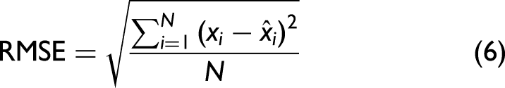

RMSE = \sqrt{\frac{\sum_{i = 1}^{N} (x_{i} - {\hat{x}}_{i})^{2}}{N}}

(6)

is a representation of the difference between the observed (

x_{i}

) and predicted (

{\hat{x}}_{i}

) values of

N

samples. A lower RMSE value indicates higher predictive accuracy and performance of a regression model. MAE, defined by Eq. 7:

MAE = \frac{\sum_{i = 1}^{N} | x_{i} - {\hat{x}}_{i} |}{N}

(7)

provides another error metric based on the absolute distance between observations and model predictions.

Furthermore, LOD is defined as the IUPAC standard representing the minimum quantity of analyte that must be present in the sample for the regression to distinguish it from a blank sample with 99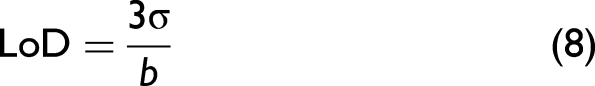 $%$ accuracy.⁵³ This metric quantifies the sensitivity of the regression model to changes in analyte concentration; a lower LOD correlates to higher sensitivity. The LOD is defined by Eq. 8:

LoD = \frac{3 σ}{b}

(8)

which quantifies the sensitivity as the ratio between the standard deviation of the blank (

σ

) to the slope of the regression (

b

). This formulation of the multivariate LOD is based on the multivariate regression fit method described in Eq. 9,

\hat{O} = a + b \times \hat{T}

(9)

where

a

and

b

represent the intercept and slope of the regression between the predicted (

\hat{O}

) and target (

\hat{T}

) points. The standard deviation of

a

yields the

σ

value for the LOD equation.

Principal component regression (PCR) and PLSR were performed on the individual LIBS and Raman data sets. Additionally, the mid-level data fusion approach depicted in Figure 4 was implemented, aggregating previously selected features from both LIBS and Raman spectra to create combined spectra for regression. As discussed in the Introduction section, data fusion methods have gained popularity in spectroscopy, as combined predictions with features from different spectroscopic methods can be more accurate than predictions made using an individual technique.

Figure 4.

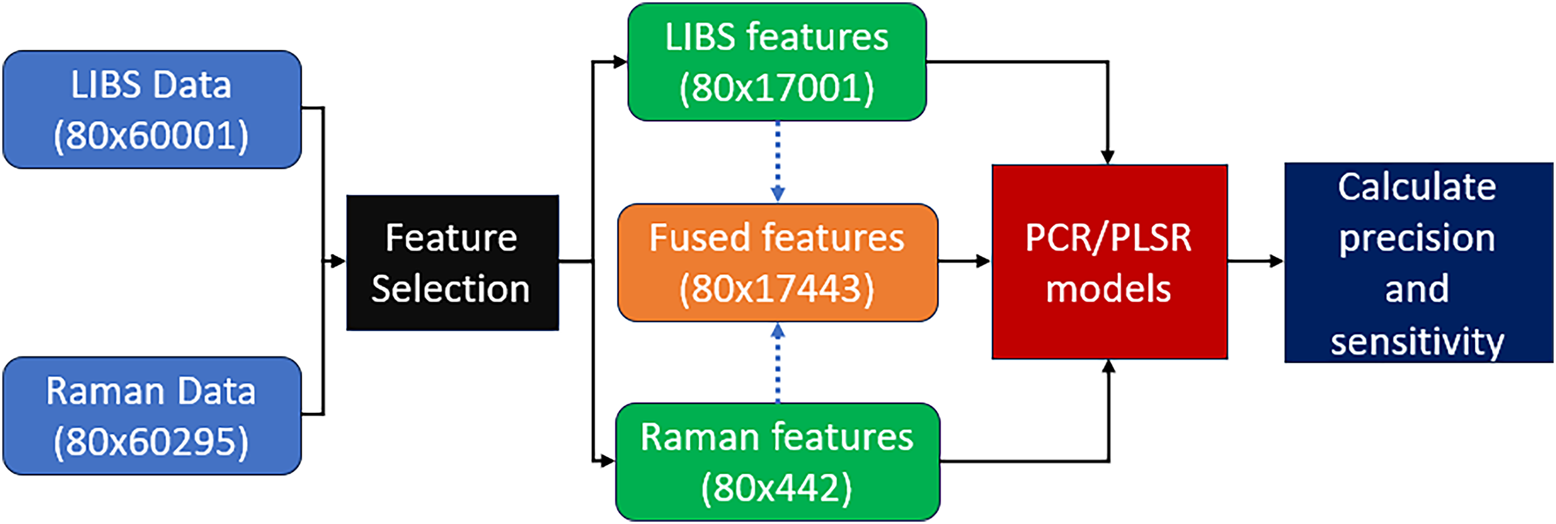
Mid-level data fusion workflow.

Machine Learning (ML) Classification Results

To begin the classification analysis, a PCA decomposition of the reduced LIBS data was done. The scores for the first three PC, which explain a total of 94 $%$ of the variance of the data, are plotted in Figure 5 to visualize the differences in the set of transformed variables between samples. This yields a clear clustering of the 600 samples in the three-dimensional (3D) PC feature space. The distinct physical separation between each compound along the PC1 axis indicates that multivariate models can distinguish sample classes based on the provided spectral features. Note that this plot does not indicate complete discrimination between LiH and LiOH samples, as seen in the overlap between the data points of these two classes. This underscores the need to implement higher-level ML classifiers to properly distinguish the samples based on subtle changes in particular spectral features.

Figure 5.

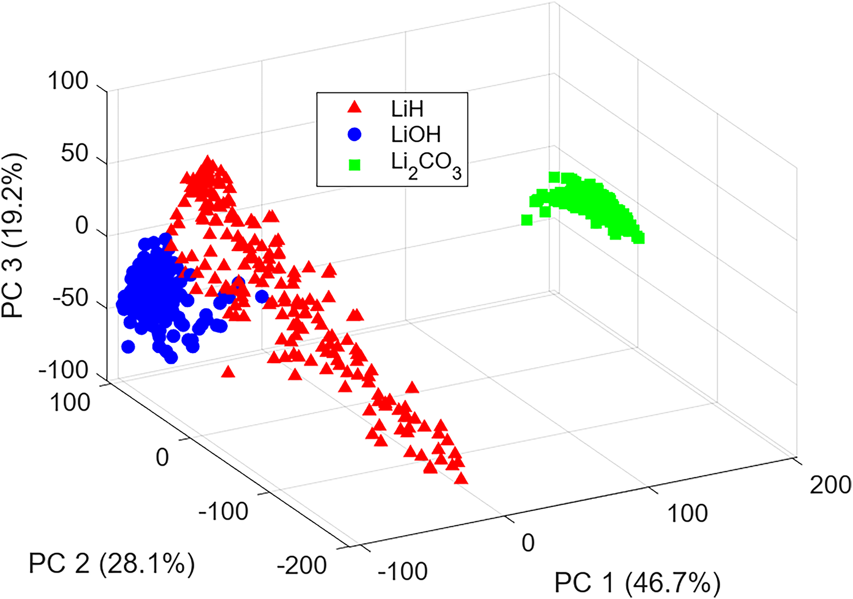
Principal component (PC) scores clustering of LiH, LiOH, and Li₂CO₃ in feature space of PCs 1–3.

The test data split was used to make predictions with each tuned classification model discussed in the Analytical Methods section. Figure 6 provides a visualization of the test classification performance of each model using confusion matrices to categorize the true and false predictions in each class. Some interesting trends can be discussed from these results. Firstly, none of the models improperly classified a spectrum of Li₂CO₃, indicating that the differences in Li₂CO₃ emission features identified in Figure 3a, particularly the lack of atomic hydrogen, are sufficiently distinct in the spectra for these samples to be easily discriminated from LiH/LiOH. The sole source of error in all four models came from misclassifying LiOH as LiH (eight occurrences) or vice-versa (one occurrence). This trend indicates that it may be more difficult for certain ML models to learn the subtle differences between the LIBS spectra of these two chemicals, which parallels the visual overlap of some LiH/LiOH data points seen in the PC clustering.

Figure 6.

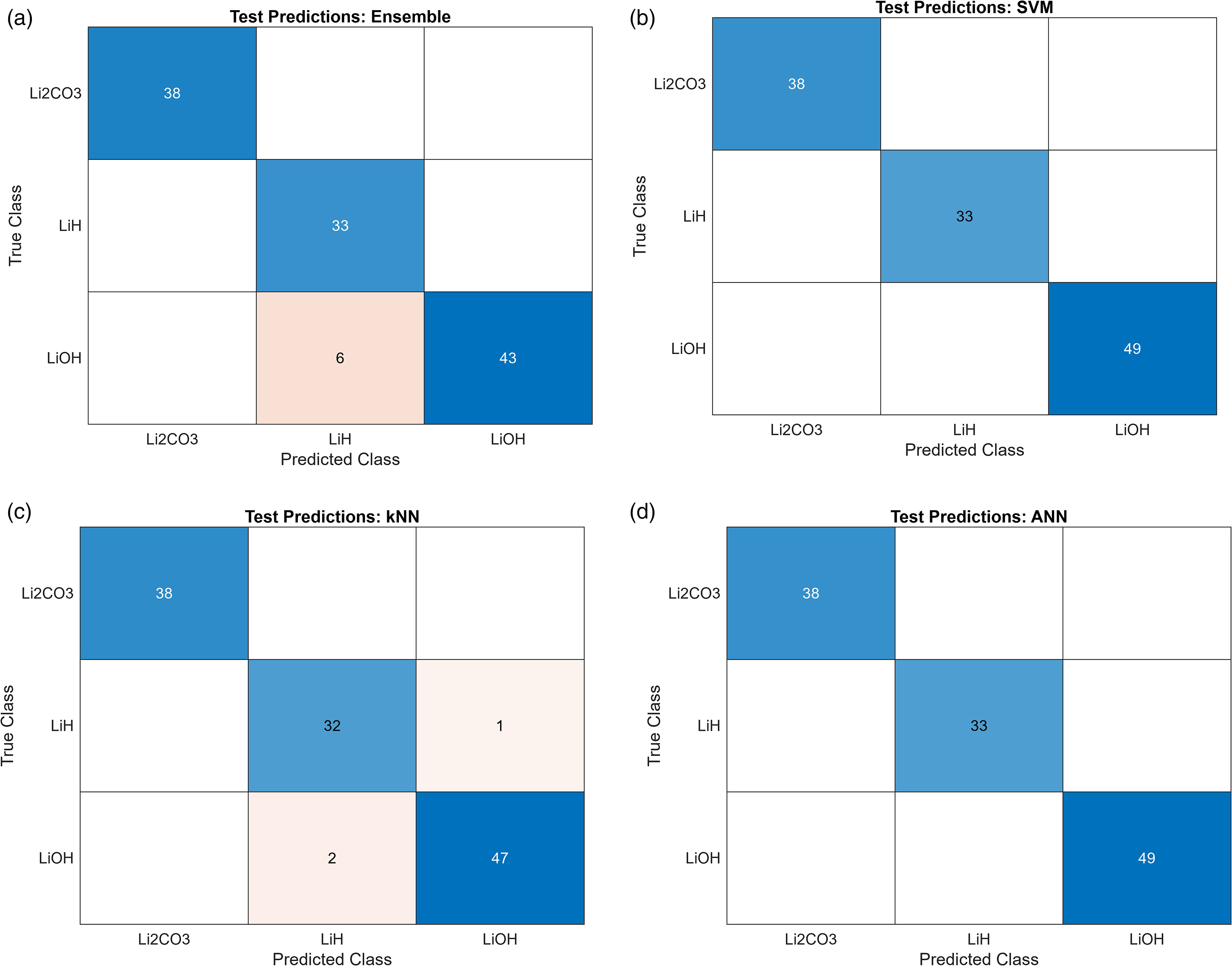
Confusion matrices for test data predictions of each tuned classifier.

Additionally, the SVM and ANN models, both known for their versatility and accuracy in classification problems, yielded perfect predictions of the test data set. This poses the question: which model is the superlative classifier if both can perfectly discriminate between these three lithium compounds? While prediction accuracy is certainly the objective, the computational cost of training a model is another factor to be evaluated in data science problems. Small gains in performance from one model to the next may not be worth the difference in the time it takes for the model to be trained, particularly when computational resources are limited or costly. Table III contrasts the test classification accuracy of each model with the training time recorded by Matlab. These metrics provide clear evidence of the computational cost of models that rely on more complex structures, as the ensemble and ANN classifiers took an order of magnitude more time to train than the SVM and KNN classifiers.

Table III.

Classification accuracy and training time of each tuned ML model.

Model	Ensemble	SVM	KNN	ANN
Accuracy ( $%$ )	95	100	97.5	100
Training time (s)	5215	470.4	440.4	6346

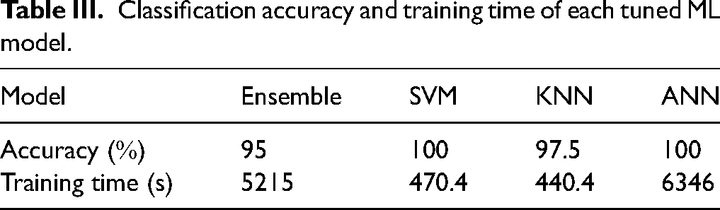
Even though the ANN made perfect test predictions, it took the longest time to generate the trained model, indicating potential impracticality for applying ANNs to classification problems with high-resolution spectral data. The tuned SVM clearly provides the superlative model, yielding the same result as the ANN with 13 $\times$ less training time.

Multivariate Regression Results

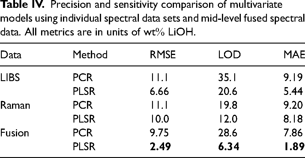
Regressions predicting LiOH content in LiH were constructed with 10-component PCR and PLSR as per Figure 4. Figures 7a and b show the regression results using the pre-processed LIBS and Raman data sets individually. As expected, PCR performs worse than PLSR with far less linearity and larger error because it is an unsupervised learning technique. LOD calculated for each model is listed in Table IV with the best performance parameters bolded; overall, the results indicate poor model generalization, predictive capability, and sensitivity when data from the two spectroscopic methods are used individually to create a multivariate regression. 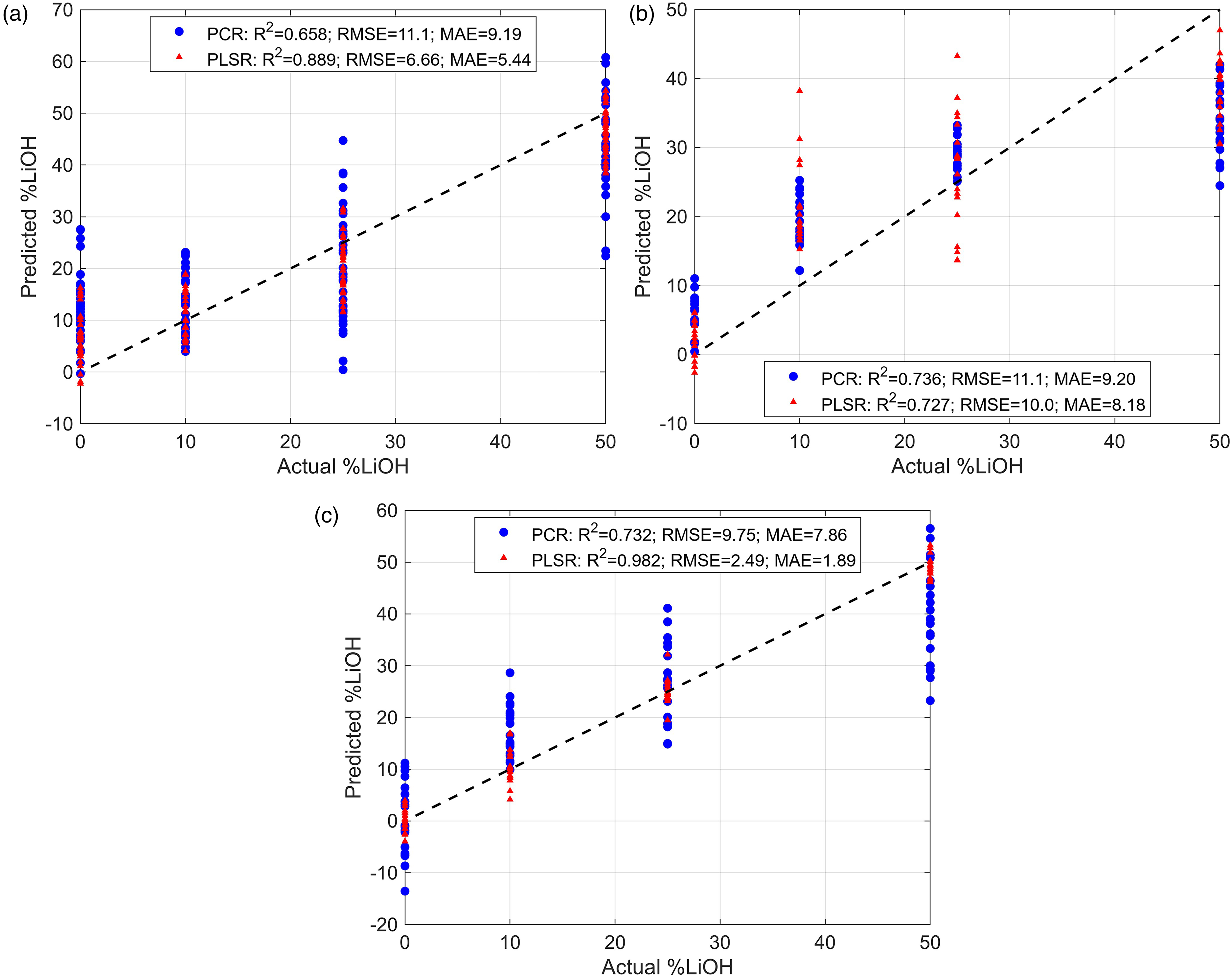However, the fused data regressions show marked improvement in regression fidelity; the PLSR model in particular yielded the lowest RMSE of 2.49 wt $%$ and the lowest LOD of 6.34 wt $%$ . The improvement in these metrics is visually reflected in Figure 7c, noting that the dispersion in the prediction points across the entire range is much lower, hence the increased accuracy. The dispersion of the $y$ -intercept of the fused PLSR model is also much less than what manifests in the other five models; a lower intercept dispersion correlates to a lower $σ$ value, hence a lower LOD.

Figure 7.

Principal component regression (PCR) and PLSR results using (a) LIBS, (b) Raman, and (c) fused feature data sets.

Table IV.

Precision and sensitivity comparison of multivariate models using individual spectral data sets and mid-level fused spectral data. All metrics are in units of wt $%$ LiOH.

Data	Method	RMSE	LOD	MAE
LIBS	PCR	11.1	35.1	9.19
	PLSR	6.66	20.6	5.44
Raman	PCR	11.1	19.8	9.20
	PLSR	10.0	12.0	8.18
Fusion	PCR	9.75	28.6	7.86
	PLSR	2.49	6.34	1.89

The regression analysis conducted with the data set, albeit simple in concept, highlights several important points for future endeavors in performing similar analysis. Differences in recorded spectra between samples with small differences in LiOH concentration can be difficult to generalize with basic multivariate models. To push the state-of-the-art and develop truly high-fidelity models, it is imperative to expand the scale of the collected data and the number of different chemical mixtures used in the experiment. Having a larger data set with more concentration points will enable higher-level ML methods, such as those discussed in the ML Classification Results section, to be used in the construction of better regression models. This will enable the construction of models that can better learn the relationship between spectral feature changes and analyte content, and allow for further experimentation with data fusion methodologies to reduce prediction error and model sensitivity.

Conclusion

This work demonstrated the efficacy of a tandem LIBS–Raman spectroscopy setup for the analysis of lithium compounds (LiH, LiOH, and Li₂CO₃). SVM classification using LIBS data of the three compounds provided a perfectly accurate discrimination model with a relatively low computational training cost. A mid-level data fusion methodology, combining selected features from individual LIBS and Raman spectra, was able to quantify LiOH in LiH with a prediction error as low as 2.5 $%$ and a LOD of 6.3 $%$ . This novel approach to quantifying the ingrowth of secondary lithium compounds has great potential as a quality assurance tool for lithium manufacturing industries. The results and research presented in this paper lay the foundations for future studies of this tandem LIBS–Raman approach which can integrate advanced supervised ML techniques to further reduce error and detection limits. Combining higher-level data fusion approaches with optimized ML regressions could potentially allow for the reduction of LODs down to tens of parts per million (ppm) as demonstrated in recent studies of complex actinide alloys.^54,55 The performance improvements seen with the simple PLSR technique using a basic fusion approach indicate that more promising improvements could be developed in expanded investigations.

Supplemental Material

sj-pdf-1-asp-10.1177_00037028241235679 - Supplemental material for Analysis of Lithium Aging Using Machine Learning-Enhanced Spectroscopy Techniques

Supplemental material, sj-pdf-1-asp-10.1177_00037028241235679 for Analysis of Lithium Aging Using Machine Learning-Enhanced Spectroscopy Techniques by James T. Stofel, Ashwin P. Rao, Anil K. Patnaik, Andrew V. Giminaro, and Michael B. Shattan in Applied Spectroscopy

Footnotes

Declaration of Conflicting Interests

The authors declared no potential conflicts of interest with respect to the research, authorship, and/or publication of this article.

Funding

The authors disclosed receipt of the following financial support for the research, authorship, and/or publication of this article: This work was funded by the Defense Threat Reduction Agency’s Nuclear Science and Engineering Research Center. Distribution Unlimited; approved for public release under cases 88ABW-2021-0154 and AFRL-2023-6449. The views expressed are those of the authors and do not necessarily reflect the official policy or position of the Department of the Air Force, the Department of Defense, or the U.S. government.

ORCID iDs

James T. Stofel

Ashwin P. Rao

Anil K. Patnaik

Supplemental Material

All supplemental material mentioned in the text is available in the online version of the journal.

References

Nazri

G.A.

Aymard

Oumellal

Rougier

Tarascon

J.-M.

. Lithium Hydride Negative Electrode for Rechargeable Lithium Batteries. US Patent 7736805B2. Filed 2007. Issued 2010.

WebMD . "Lithium Carbonate". https://www.webmd.com/drugs/2/drug-5887-42/lithium-carbonate-oral/lithium-oral/details [accessed Jan 30 2021].

Welch

F.H.

. “Lithium Hydride: A Space Age Shielding Material”. Nucl. Eng. Des. 1974. 26(3): 444–460.

Han

Wang

Zhao

et al. “Efficient Neutron Radiation Shielding by Boron–Lithium Imidazolate Frameworks”. Dalton Trans. 2022. 51(31): 11625–11629.

Cox

S.O.

. "Criteria for the Safe Storage of Lithium Metal and Lithium Compounds at the Y-12 Plant". https://www.osti.gov/servlets/purl/162490 [accessed Feb 26 2024].

Johnson Jr

A.B.

., Kabele

T.J.

Gurwell

W. E.

. "Tritium Production From Ceramic Targets: A Summary of the Hanford Coproduct Program". https://www.osti.gov/servlets/purl/7125831 [accessed Feb 26 2024].

McDonell

W.R.

. "Aluminum–Lithium Target Behavior". Technical Report. Aiken, South Carolina: Westinghouse Savannah River Co., 1989.https://sti.srs.gov/fulltext/WSRC-RP-89-970.pdf [accessed Feb 26 2024].

Giegerich

Day

Knitter

Osman

. "Lithium Enrichment Issues in the Sustainable Supply Chain of Future Fusion Reactors". First IAEA Technical Meeting (TM) on the Safety, Design, and Technology of Fusion Power Plants. International Atomic Energy Agency (IAEA) Headquarters. Vienna, Austria, 3-5 May 2016.

Chadwick

Obložinskỳ

Herman

Greene

N.M.

, et al. “ENDF/B-VII.0: Next Generation Evaluated Nuclear Data Library for Nuclear Science and Technology”. Nucl. Data Sheets. 2006. 107(12): 2931–3060.

10.

Williams

Miller

. “Effect of Water Vapor on the LiOH-CO₂ Reaction. Dynamic Isothermal System”. Ind. Eng Chem. Fund. 1970. 9(3): 454–457.

11.

Haertling

Hanrahan Jr

Smith

. “A Literature Review of Reactions and Kinetics of Lithium Hydride Hydrolysis”. J. Nucl. Mater. 2006. 349(1-2): 195–233.

12.

Sifuentes

Stowe

A.C.

Smyrl

. “Determination of the Role of Li₂O on the Corrosion of Lithium Hydride”. J. Alloys Compd. 2013. 580: S271–S273. https://doi.org/10.1016/j.jallcom.2013.02.046

13.

Ponzio

Woodward

Stowe

A.C.

. “Investigation of Oxidation Surface Reactions on LiH Utilizing Laser Induced Breakdown Spectroscopy (LIBS)”. Consolidated Nuclear Security, LLC, Y-12 National Security Complex and Pantex Plant, October 2014.

14.

Stowe

A.C.

Smyrl

. “Raman Spectroscopy of Lithium Hydride Corrosion: Selection of Appropriate Excitation Wavelength to Minimize Fluorescence”. Vib. Spectrosc. 2012. 60: 133–136. https://doi.org/10.1016/j.vibspec.2012.01.018

15.

Gorelik

V.S.

Voinov

Y.P.

Vodchits

A.I.

, et al. “Raman Spectra of Lithium Compounds”. J. Phys.: Conf. Ser. 2017. 918(1): 0–0. https://doi.org/10.1088/1742-6596/918/1/012035

16.

Maupoix

Houzelot

J.L.

Sciora

Gaillard

, et al. “Experimental Investigation of the Grain Size Dependence of the Hydrolysis of LiH Powder”. Powder Technol. 2011. 208: 318–323. https://doi.org/10.1016/j.powtec.2010.08.023

17.

Anderson

Luty

. “Raman Scattering, Defect Luminescence, and Phonon Spectra of Li₇H, Li₆H, and Li₇D Crystals”. Phys. Rev. B. 1983. 28(6): 3415–3421. https://doi.org/10.1103/PhysRevB.28.3415

18.

Brooker

M.H.

Wang

. “Raman and Infrared Studies of Lithium and Cesium Carbonates”. Spectrochim. Acta, Part A. 1992. 48(7): 999–1008. https://doi.org/10.1016/0584-8539(92)80176-W

19.

Wood

J.C.

Shattan

M.B.

. “Lithium Isotope Measurement Using Laser-Induced Breakdown Spectroscopy and Chemometrics”. Appl. Spectrosc. 2021. 75(2): 199–207. https://doi.org/10.1177/0003702820953205

20.

Pinson

R.E.

Giminaro

A.V.

Dugan

C.L.

Jenkins

P.R.

Patnaik

A.K.

. “LIBS and Raman Spectroscopy in Tandem With Machine Learning for Interrogating Weatherization of Lithium Hydride”. Appl. Opt. 2023. 62(6): A118–A126.

21.

Pořízka

Kaski

Hrdlička

Modlitbová

, et al. “Detection of Fluorine Using Laser-induced Breakdown Spectroscopy and Raman Spectroscopy”. J. Anal. At. Spectrom. 2017. 32: 1966–1974. https://doi.org/10.1039/C7JA00200A

22.

Eum

Jang

Lee

Cha

Chung

. “Alternative Selection of Raman or LIBS Spectral Information in Hierarchical Discrimination of Raw Sapphires According to Geographical Origin for Accuracy Improvement”. Talanta. 2021. 221: 121555. https://doi.org/10.1016/j.talanta.2020.121555

23.

Sharma

S.K.

Misra

A.K.

Lucey

P.G.

Lentz

R.C.F.

. “A Combined Remote Raman and Libs Instrument for Characterizing Minerals With 532 nm Laser Excitation”. Spectrochim. Acta, Part A. 2009. 73(3): 468–476.

24.

Gasda

P.J.

Acosta-Maeda

T.E.

Lucey

P.G.

Misra

A.K.

, et al. “Next Generation Laser-Based Standoff Spectroscopy Techniques for Mars Exploration”. Appl. Spectrosc. 2015. 69(2): 173–192. https://doi.org/10.1366/14-07483

25.

Botto

Campanella

Legnaioli

Lezzerini

, et al. “Applications of Laser-induced Breakdown Spectroscopy in Cultural Heritage and Archaeology: A Critical Review”. J. Anal. At. Spectrom. 2019. 34: 81–103. https://doi.org/10.1039/C8JA00319J

26.

Harmon

R.S.

Hark

Throckmorton

C.S.

Plumer

J.R.

, et al. "Fusion of Spectral Data From Multiple Handheld Analyzers (LIBS, XRF, and Raman) for Chemical Analysis and Classification of Soil". https://erdc-library.erdc.dren.mil/jspui/bitstream/11681/38061/1/ERDC-CRREL%20CR-20-1.pdf [accessed Feb 26 2024].

27.

Gibbons

Léveillé

Berlo

. “Data Fusion of Laser-induced Breakdown and Raman Spectroscopies: Enhancing Clay Mineral Identification”. Spectrochim. Acta, Part B. 2020. 170: 105905.

28.

Rammelkamp

Schröder

Kubitza

Vogt

D.S.

, et al. “Low-Level LIBS and Raman Data Fusion in the Context of in Situ Mars Exploration”. J. Raman Spectrosc. 2020. 51(9): 1682–1701. https://doi.org/10.1002/jrs.5615

29.

Manrique-Martinez

J.A.

Lopez-Reyes

Alvarez-Perez

Bozic

, et al. “Evaluation of Multivariate Analyses and Data Fusion Between Raman and Laser-induced Breakdown Spectroscopy in Binary Mixtures and its Potential for Solar System Exploration”. J. Raman Spectrosc. 2020. 51(9): 1702–1717. https://doi.org/10.1002/jrs.5819

30.

Gibbons

Léveillé

Berlo

. “Data Fusion of Laser-induced Breakdown and Raman Spectroscopies: Enhancing Clay Mineral Identification”. Spectrochim. Acta, Part B. 2020. 170: 105905. https://doi.org/10.1016/j.sab.2020.105905

31.

Xue

Zhang

. “Data Fusion of Raman and Near-Infrared Spectroscopies for the Rapid Quantitative Analysis of Methanol Content in Methanol–Gasoline”. Energy Fuels. 2019. 33(12): 12286–12294.

32.

Rao

A.P.

Jenkins

P.R.

Pinson

R.E.

Auxier II

J.D.

, et al. “Machine Learning in Analytical Spectroscopy for Nuclear Diagnostics”. Appl. Opt. 2023. 62(6): A83–A109.

33.

Shameem

K.M.M

Dhanada

V.S.

Harikrishnan

George

S.D.

, et al. “Echelle LIBS–Raman System: A Versatile Tool for Mineralogical and Archaeological Applications”. Talanta. 2020. 208(120482): 1–11. https://doi.org/10.1016/j.talanta.2019.120482

34.

Guezenoc

Gallet-Budynek

Bousquet

. “Critical Review and Advices on Spectral-Based Normalization Methods for LIBS Quantitative Analysis”. Spectrochim. Acta, Part B. 2019. 160: 105688. https://doi.org/10.1016/j.sab.2019.105688

35.

Syvilay

Wilkie-Chancellier

Trichereau

Texier

, et al. “Evaluation of the Standard Normal Variate Method for Laser-Induced Breakdown Spectroscopy Data Treatment Applied to the Discrimination of Painting Layers”. Spectrochim. Acta, Part B. 2015. 114: 38–45. https://doi.org/10.1016/j.sab.2015.09.022

36.

Heraud

Wood

B.R.

Beardall

McNaughton

. “Effects of Pre-Processing of Raman Spectra on in Vivo Classification of Nutrient Status of Microalgal Cells”. J. Chemom. 2006. 20(5): 193–197. https://doi.org/10.1002/cem.990

37.

Guo

Kokot

. “Evaluation of Chemical Components and Properties of the Jujube Fruit Using Near Infrared Spectroscopy and Chemometrics”. Spectrochim. Acta, Part A. 2016. 153: 79–86. https://doi.org/10.1016/j.saa.2015.08.006

38.

Liu

K.H.

Gao

Feng

K.J.

, et al. “A Novel Soft-Coded Error-Correcting Output Codes Algorithm”. Pattern Recognit. 2023. 134: 109122. https://doi.org/10.1016/j.patcog.2022.109122

39.

Larose

. Data Mining and Predictive Analysis. Hoboken, New Jersey: Wiley, 2015.

40.

Rokach

Maimon

. Data Mining with Decision Trees. Hackensack, New Jersey: World Scientific Publishing Company, 2007.

41.

Haykin

. Neural Networks: A Comprehensive Foundation. Hoboken, New Jersey: Prentice Hall, 1999.

42.

Laaksonen

Oja

. "Classification With Learning k-Nearest Neighbors". In: Proceedings of International Conference on Neural Networks (ICNN’96), 1996. Pp. 1480–1483. https://doi.org/10.1109/ICNN.1996.549118.

43.

Cho

Kim

Lee

Choi

, et al. “Basic Enhancement Strategies When Using Bayesian Optimization for Hyperparameter Tuning of Deep Neural Networks”. IEEE Access . 2020. 8: 52588–52608.

44.

Snoek

Larochelle

Adams

R.P.

. “Practical Bayesian Optimization of Machine Learning Algorithms”. Adv. Neural Inf. Process. Syst. 2012. 25: 1–9.

45.

Rao

A.P.

Jenkins

P.R.

Auxier

J.D.

Shattan

M.B.

Patnaik

A.K.

. “Development of Advanced Machine Learning Models for Analysis of Plutonium Surrogate Optical Emission Spectra”. Appl. Opt. 2022. 61(7): D30–D38.

46.

The MathWorks, Inc. "Statistics and Machine Learning Toolbox Analyze and Model Data Using Statistics and Machine Learning". https://www.mathworks.com/help/stats [accessed Feb 26 2024].

47.

Unnikrishnan

Choudhari

Kulkarni

S.D.

Nayak

, et al. “Analytical Predictive Capabilities of Laser Induced Breakdown Spectroscopy (LIBS) With Principal Component Analysis (PCA) for Plastic Classification”. RSC Adv. 2013. 3(48): 25872–25880.

48.

Erdem

Çilingiroğlu

Giakoumaki

Castanys

, et al. “Characterization of Iron Age Pottery From Eastern Turkey by Laser-induced Breakdown Spectroscopy (LIBS)”. J. Archaeol. Sci. 2008. 35(9): 2486–2494.

49.

Elmas ŞN

Arslan

F.N.

Akin

Kenar

et al. “Synchronous Fluorescence Spectroscopy Combined with Chemometrics for Rapid Assessment of Cold-Pressed Grape Seed Oil Adulteration: Qualitative and Quantitative Study”. Talanta. 2019. 196: 22–31.

50.

Oztoprak

B.G.

Gonzalez

Yoo

SNMGulecen

, et al. “Analysis and Classification of Heterogeneous Kidney Stones Using Laser-Induced Breakdown Spectroscopy (LIBS)”. Appl. Spectrosc. 2012. 66(11): 1353–1361.

51.

Martin

M.Z.

Labbé

André

Wullschleger

S.D.

, et al. “Novel Multivariate Analysis for Soil Carbon Measurements Using Laser-Induced Breakdown Spectroscopy”. Soil Sci. Soc. Am. J. 2010. 74(1): 87–93.

52.

Zhang

Mohua

Karanassios

. "Artificial Neural Networks (ANNs) for Spectral Interference Correction Using a Large-size Spectrometer and ANN-Based Deep Learning for a Miniature One". In: Aded El-Shahat, editor. Advanced Applications for Artificial Neural Networks. London, UK: InTech Publishing, 2018. Pp. 227–249. 10.5772/intechopen.71039

53.

Long

. “A Closer Look at the IUPAC Definition”. Anal. Chem. 2008. 55(7): 712A–724A https://doi.org/10.1021/ac00258a001

54.

Rao

A.P.

Jenkins

P.R.

Auxier

I.I.J.D.

Auxier II

J.D.

Shattan

M. B.

. “Comparison of Machine Learning Techniques to Optimize the Analysis of Plutonium Surrogate Material Via a Portable LIBS Device”. J. Anal. At. Spectrom. 2021. 36(2): 399–406.

55.

Rao

A.P.

Jenkins

P.R.

D.M.

Auxier II

J.D.

, et al. “Rapid Quantitative Analysis of Trace Elements in Plutonium Alloys Using a Handheld Laser-induced Breakdown Spectroscopy (LIBS) Device Coupled With Chemometrics and Machine Learning”. Anal. Methods. 2021. 13(30): 3368–3378.

Supplementary Material

Please find the following supplemental material available below.

For Open Access articles published under a Creative Commons License, all supplemental material carries the same license as the article it is associated with.

For non-Open Access articles published, all supplemental material carries a non-exclusive license, and permission requests for re-use of supplemental material or any part of supplemental material shall be sent directly to the copyright owner as specified in the copyright notice associated with the article.

0.00 MB

0.24 MB