Complex-Valued Chemometrics in Spectroscopy: Inverse Least Squares Regression

Abstract

Inverse least squares (ILS) regression is an advancement of classical least squares (CLS) regression, enabling the calculation of concentrations without requiring prior knowledge of the number of components in a mixture. Complex-valued ILS further enhances the performance of ILS by incorporating the complex refractive index function, as demonstrated in the thermodynamically ideal mixtures of benzene–toluene and benzene–cyclohexane. In both systems, the mean absolute error can be reduced by over 50% using the leave-one-out cross-validation (LVOOCV) scheme with complex-valued ILS. Additional error reduction is achievable by leveraging correlations between the errors and the imaginary components of the concentrations or volume fractions. Since the complex refractive index function can be conveniently determined using conventional infrared spectroscopy through the Kramers–Kronig relations, we believe that complex-valued machine learning has the potential to significantly advance analytical applications.

Graphical abstract

This is a visual representation of the abstract.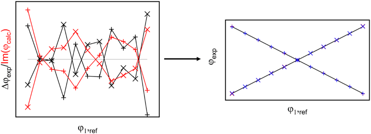

Keywords

Ideal binary liquid mixtures inverse least squares regression complex refractive index spectra

Introduction

Classical least squares (CLS) regression is a method that has been in use for over 200 years.¹ By assuming a linear relationship between absorbance and molar concentration, it became widely popular among spectroscopists for determining unknown concentrations through calibration. In the calibration process, spectra are required for a range of known concentrations for each component. This requirement becomes particularly challenging when reactions occur, as the concentrations of products and all stable intermediates would also need to be determined.

This limitation prompted the development of inverse least squares (ILS) regression about 60 years ago.² ILS inverts Beer’s Law, treating concentration as a function of absorbance. Consequently, calibration no longer requires the concentrations of every component to be known. However, to fully utilize the spectrum, one must either measure more compositions than the number of wavenumber points in the spectrum or significantly reduce the number of wavenumber points. If these remaining wavenumber points are carefully selected, ILS can outperform CLS.³

This may seem paradoxical because the main advantage of CLS lies in being a full-spectrum method that utilizes every wavenumber point, whereas ILS, with only a handful of well-chosen points, can surpass CLS. How is this possible? Both ILS and CLS assume that only random deviations from Beer’s law are present in the spectra. If Beer’s law held strictly, CLS would generally outperform ILS. However, Beer’s law is a limiting law and does not hold perfectly,^4,5 even for thermodynamically ideal mixtures.^6,7 When systematic errors are present, focusing on a few wavenumber points where Beer’s law approximates reality more closely proves superior to using the entire spectrum.

Selecting optimal wavenumber points can be extremely challenging, leading to the development of various methods to address this issue.² One alternative is compressing spectral data and employing techniques such as principal component regression or partial least squares regression. An intriguing but less commonly used approach for data compression is integrating absorbance spectra.³ This method bears a strong resemblance to the refractive index function, which increases with decreasing wavenumber in proportion to the area of absorption index bands at higher wavenumbers.^5,8,9 As a result, selecting favorable wavenumber points becomes significantly easier when refractive index spectra are used for calibration.

While refractive index spectra might appear difficult to obtain, modern techniques such as spectroscopic ellipsometry can measure the complex refractive index function.¹⁰ This function is also routinely derived from attenuated total reflection (ATR) spectroscopy, which requires corrections equivalent to determining the complex refractive index.^11–16 Corrections are not limited to ATR spectra; they are also necessary for transmission and transflection spectra.^17–19 Emerging methods, such as infrared refraction and dispersion spectroscopy and field-resolved infrared spectroscopy, further facilitate the direct measurement of the refractive index function.^20–26

Recently, we introduced spectroscopic complex-valued CLS regression.^27,28 This technique demonstrated a distinct advantage when using the complex refractive index function compared to employing only its real or imaginary part. However, this advantage did not emerge merely from substituting the complex refractive index function into the CLS formulas. An additional step was required, leveraging the fact that concentrations must be real-valued functions. The resulting imaginary components of the concentrations were found to correlate with calibration errors, enabling error reduction when determining the unknown concentration of a sample.²⁸

In this study, we investigate whether such an indirect error reduction approach is also applicable to ILS regression or whether complex-valued ILS can directly reduce the sum of the absolute mean error, unlike complex-valued CLS.

Theoretical Aspects

The close proximity of neighboring molecules in condensed matter results in interactions where the polarization of one molecule by a photon may induce polarization in adjacent molecules. This interaction introduces nonlinearity into the system. When a molecule with spherical symmetry is surrounded by other symmetrically arranged molecules, the Lorentz–Lorenz equation may be applicable. This equation, formulated independently by L. Lorenz in 1867 and H.A. Lorentz in 1878, explains how the refractive index of mixtures can be determined from the refractive indices of the individual pure substances:^29–31

\frac{{\hat{n}}^{2} - 1}{{\hat{n}}^{2} + 2} = \sum_{i} \frac{{\hat{n}}_{i}^{2} - 1}{{\hat{n}}_{i}^{2} + 2} φ_{i}

(1)

In this equation,

{\hat{n}}_{i}

represents the complex refractive index of pure component i, comprising a real part n_i and an imaginary part k_i (where k is the absorption coefficient) and is its volume fraction

φ_{i}

.^13,24 Eq. 1 presumes that the mixture behaves as an ideal thermodynamic system, maintaining constant molar volumes upon mixing:

\sum_{i} φ_{i} = 1

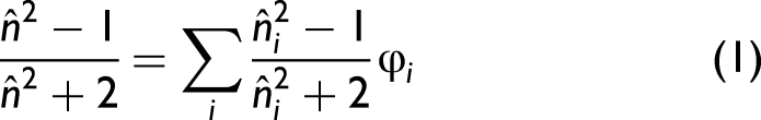
In scenarios where the oscillator strength is minimal (k << 1 and n ≈ 1),

\begin{aligned} {\hat{n}}^{2} + 2 \approx 3 \\ {\hat{n}}^{2} - 1 \approx 2 (\hat{n} - 1) \end{aligned}

and similar relations hold for the pure components, the Lorentz–Lorenz relation simplifies to³²

\hat{n} - 1 = \sum_{i} ({\hat{n}}_{i} - 1) φ_{i}

(2)

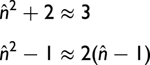
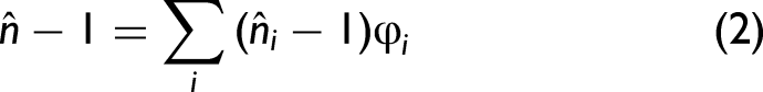
The refractive index varies with frequency, wavelength, or wavenumber and is a complex variable.

Assume that we have conducted m measurements, each yielding a complex refractive index spectrum $\hat{n} (\tilde{ν})$ with l discrete wavenumber points for mixtures containing j components. Each measurement corresponds to m different volume fractions for the j components. In this context, Eq. 2 can be expressed using the spectra of the components as follows:^27,28

\hat{n} = φ \hat{K}

(3)

From the measured spectra, we can compute the matrix

\hat{n}

and, if the volume fractions of all components in each mixture are known, the matrix φ. The matrix

\hat{K}

consists of the spectra of the pure components. Assuming that Beer’s approximation is applicable, but the correct number of components is unknown, an inverse approach might be used. In this approach, we hypothesize that:

φ = \hat{n} {\hat{P}}_{I L S}

(4)

where

{\hat{P}}_{I L S}

does not possess an obvious physical significance. It can be calculated as follows:

{\hat{P}}_{I L S} = ({\hat{n}}^{T} \hat{n})^{- 1} {\hat{n}}^{T} φ

(5)

This calculation enables us to determine the unknown composition φ _u from the complex refractive index spectrum

\hat{n} (\tilde{ν}) = {\hat{n}}_{u}

by:

φ_{u} = {\hat{n}}_{u} {\hat{P}}_{I L S}

(6)

It is important to note that since matrix $\hat{n}$ contains complex entries, taking its transpose may also require taking the complex conjugate. If matrix $\hat{n}$ were to encapsulate the full spectra, the formalism would become ill-conditioned when the number of independent spectra is fewer than the wavenumber points. Therefore, matrix $\hat{n}$ should be limited to no more entries than the number of measurements, or fewer.

Experimental

Materials and Methods

Fourier transform infrared (FT-IR) spectra of benzene-toluene mixtures with toluene volume fractions from 0 to 1 (φ₁ = 0, 0.1, 0.2 …1) were obtained using a Thermo Scientific Nicolet iS50 FT-IR spectrometer, which features an integrated diamond ATR accessory. The measurements covered a spectral range of 400–4000 cm⁻¹ at a resolution of 4 cm⁻¹, later interpolated to 0.5 cm⁻¹. For further details, refer to the supporting information and Mayerhöfer et al.⁶ The spectra were corrected using an advanced ATR correction method as described in Mayerhöfer et al.¹³ The values for n_∞ for pure benzene and toluene were taken from Myers et al.,³³ for the mixtures n_∞ was computed using Eq. 1. For cyclohexane, n_∞ was extrapolated based on experimental values from the visible spectrum taken from Myers et al.³³ as per the Sellmeier equation. No additional spectral manipulation, commonly referred to as “spectral preprocessing”, was performed, adhering to the principles of wave optics.

Results and Discussion

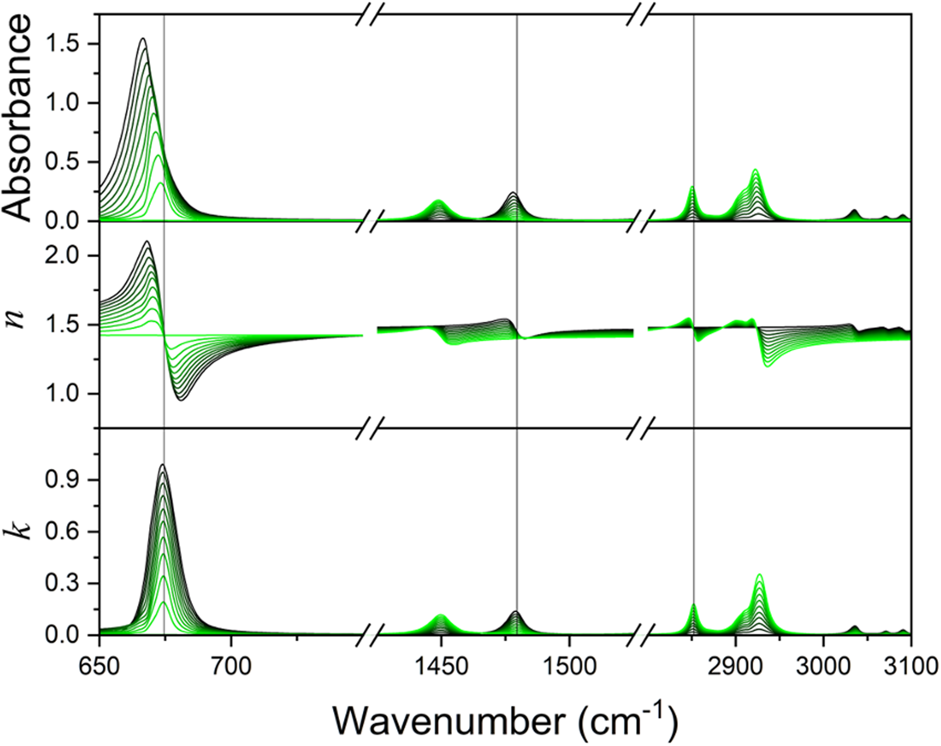
Figure 1 shows the spectra recorded for the benzene–toluene system, along with the wavenumber points selected for ILS (the raw spectra as well as the n- and k-spectra are provided as Supplemental Material). Selecting these points is relatively straightforward for absorbance and absorption index spectra, as wavenumber points in non-absorbing regions do not contribute. However, due to peak shifts in these spectra and the question of how many points to choose, the selection process remains non-trivial.

Figure 1.

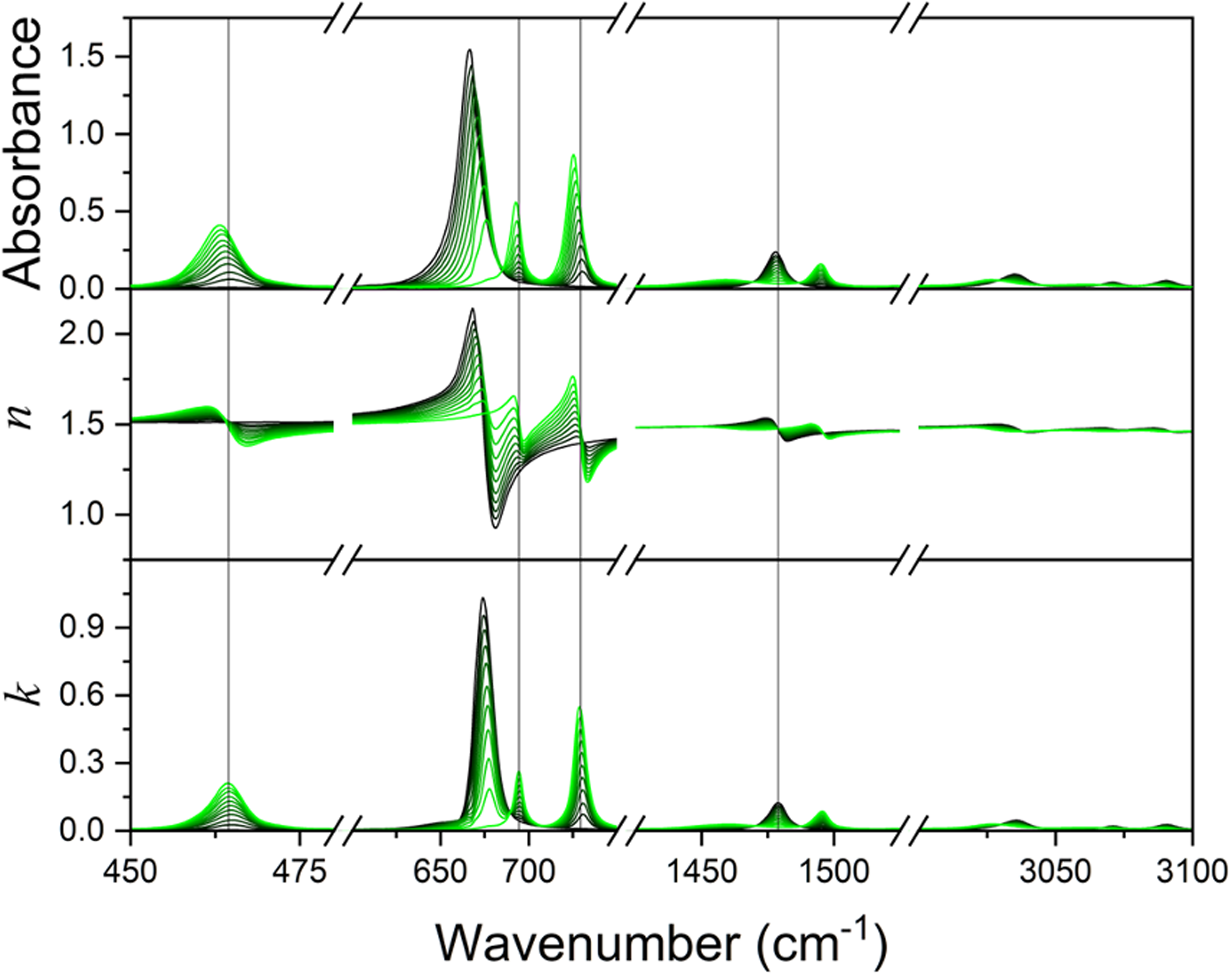
Selected wavenumber ranges of the ATR, n- and k-spectra of the system benzene–toluene. The wavenumber points chosen for ILS are indicated by vertical lines.

One might assume that selecting as many points as possible would be advantageous. However, using the mean absolute error (MAE) or, alternatively, the root mean squared error (RMSE) from the “leave-one-out” scheme of ILS as a guide, we arrived at selecting only four points. While we cannot claim that this choice leads to the absolute minimum of the MAE and the RMSE, we are confident that some form of error compensation is at play, as the results are significantly better than those obtained from CLS (see Mayerhöfer et al.²⁸). The selection of these points began by identifying the peak positions in the k-spectra of the pure components. We then systematically removed individual peaks and retained their exclusion if it resulted in a lower MAE. In the following, we focus on the MAEs. MAE was given preference because it provides a direct and interpretable measure of average prediction error without disproportionately emphasizing large deviations, as RMSE does. However, for completeness, we also report RMSE values alongside MAE in Tables I and II. Overall, RMSE and MAE yielded comparable results. After determining the final number of peaks, we fine-tuned the wavenumber positions in 0.5 cm⁻¹ increments. However, for k-spectra, the MAE typically reaches a minimum at or very close to the original peak positions.

Table I.

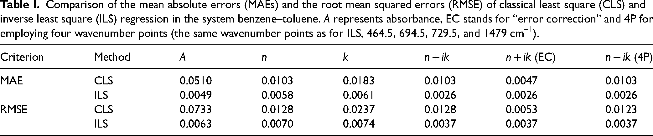
Comparison of the mean absolute errors (MAEs) and the root mean squared errors (RMSE) of classical least square (CLS) and inverse least square (ILS) regression in the system benzene–toluene. A represents absorbance, EC stands for “error correction” and 4P for employing four wavenumber points (the same wavenumber points as for ILS, 464.5, 694.5, 729.5, and 1479 cm^–1).

Criterion	Method	A	n	k	n + ik	n + ik (EC)	n + ik (4P)
MAE	CLS	0.0510	0.0103	0.0183	0.0103	0.0047	0.0103
MAE	ILS	0.0049	0.0058	0.0061	0.0026	0.0026	0.0026
RMSE	CLS	0.0733	0.0128	0.0237	0.0128	0.0053	0.0123
RMSE	ILS	0.0063	0.0070	0.0074	0.0037	0.0037	0.0037

Table II.

Comparison of the mean absolute errors (MAEs) and the root mean squared errors (RMSE) of classical least square (CLS) and inverse least square (ILS) regression in the system benzene–cyclohexane.

Criterion	Method	Absorbance	n	k	n + ik	n + ik (EC)^a
MAE	CLS	0.0551	0.0170	0.0131	0.0168	0.0098
MAE	ILS	0.0093	0.0050	0.0046	0.0025	0.0019
RMSE	CLS	0.0882	0.0229	0.0201	0.0227	0.0140
RMSE	ILS	0.0134	0.0058	0.0068	0.0030	0.0024

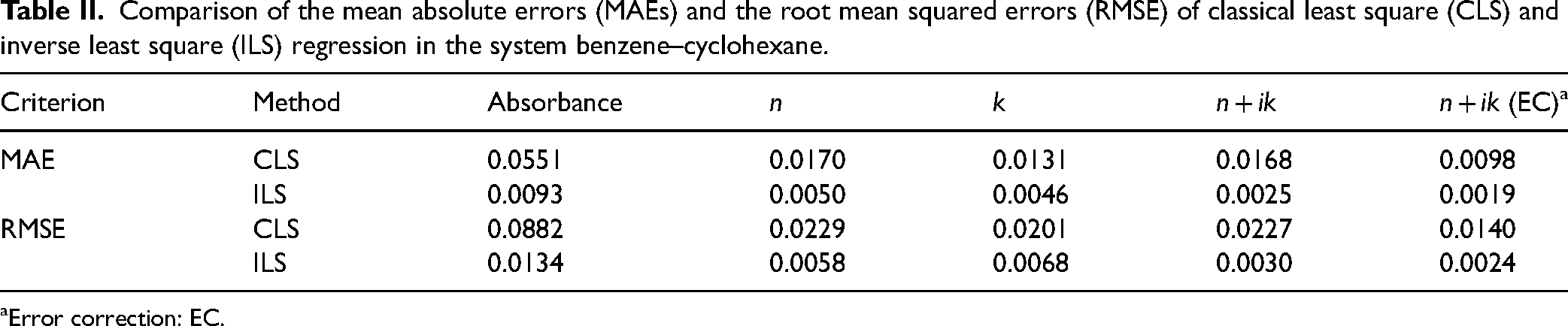
^aError correction: EC.

We decided to use the same four wavenumber points for both the refractive index and complex refractive index spectra, namely 464.5, 694.5, 729.5, and 1479 cm^–1, acknowledging that this selection is far from ideal, particularly for the refractive index spectra. This is evident in Figure 1, where the selected points predominantly correspond to regions where changes in the refractive index with the volume fraction are minimal. Notably, shifting one of these wavenumber points by 0.5 or 1 cm⁻¹ towards spectral regions with stronger changes has a significant impact on the MAE. Despite this, the MAE value of 0.0058 achieved with the refractive index spectra was slightly smaller than the 0.0061 obtained using the absorption index spectra (cf. Table I).

In contrast, the MAE resulting from performing ILS with the complex refractive index spectra was only 0.0030, less than half that of the absorption index spectra.

To compare the results of CLS with those of ILS, it is noteworthy that without the additional correction mechanism, CLS based on the complex or real refractive index yielded a MAE of 0.0103,²⁸ cf. Table I. This value was reduced to 0.0047 when complex-valued CLS was applied, incorporating the correction mechanism.²⁸ This mechanism adjusted the imaginary parts of the volume fractions by multiplying them with a common factor to align these parts with the calibration errors. This allows removing this error from the real part as we will explain later in more details.

In contrast, ILS achieved a MAE of 0.0030 without applying any additional correction mechanism. With some minor adjustments using the points at 463, 694, 729, and 1479 cm^–1, the MAE for ILS could be further reduced to 0.0027 (Table I). Accidentally, when complex-valued CLS is applied using only these four wavenumber points, the resulting MAE is identical to that obtained using the full spectrum, whereas the results based solely on the k- or n-spectra are significantly worse (cf. Table S1 and Figure S1, Supplemental Material). This demonstrates that even with a limited number of points, complex-valued CLS offers a clear advantage over conventional CLS. However, in this case, the error correction based on the imaginary part of the volume fraction fails, likely because the nature of the nonlinearity cannot be adequately captured with so few points. The performance difference between CLS and ILS arises for the same reason as in the full-spectrum case: CLS assumes a two-component system, while ILS does not, allowing greater flexibility in modeling deviations from linearity.

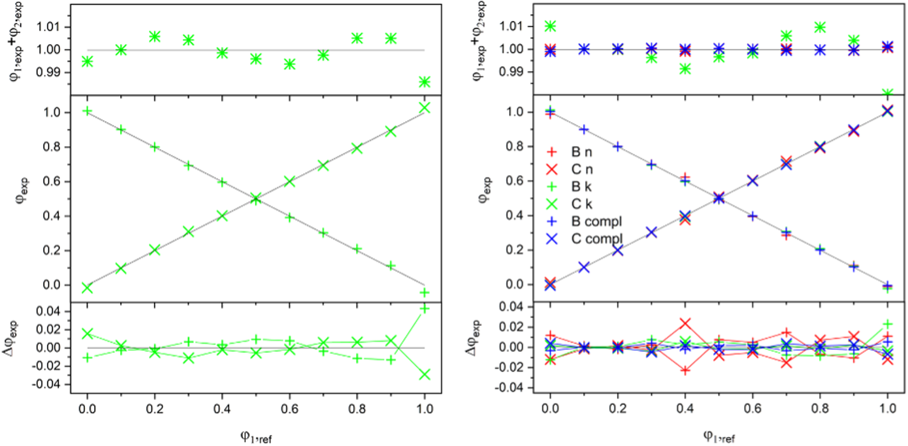
Notably, applying ILS reduces the MAE compared to CLS by half, resulting in a value of 0.0049 when applied to uncorrected spectra using the same four wavenumber points. This is smaller than the MAE obtained using the absorption index function (see Table I and the left panel of Figure 2). However, errors remain evident when inspecting the sum of the volume fractions, which typically deviate by about 1%. This deviation becomes much smaller when either the real or the complex refractive index function is used. The program we used for ILS is available as supporting information.

Figure 2.

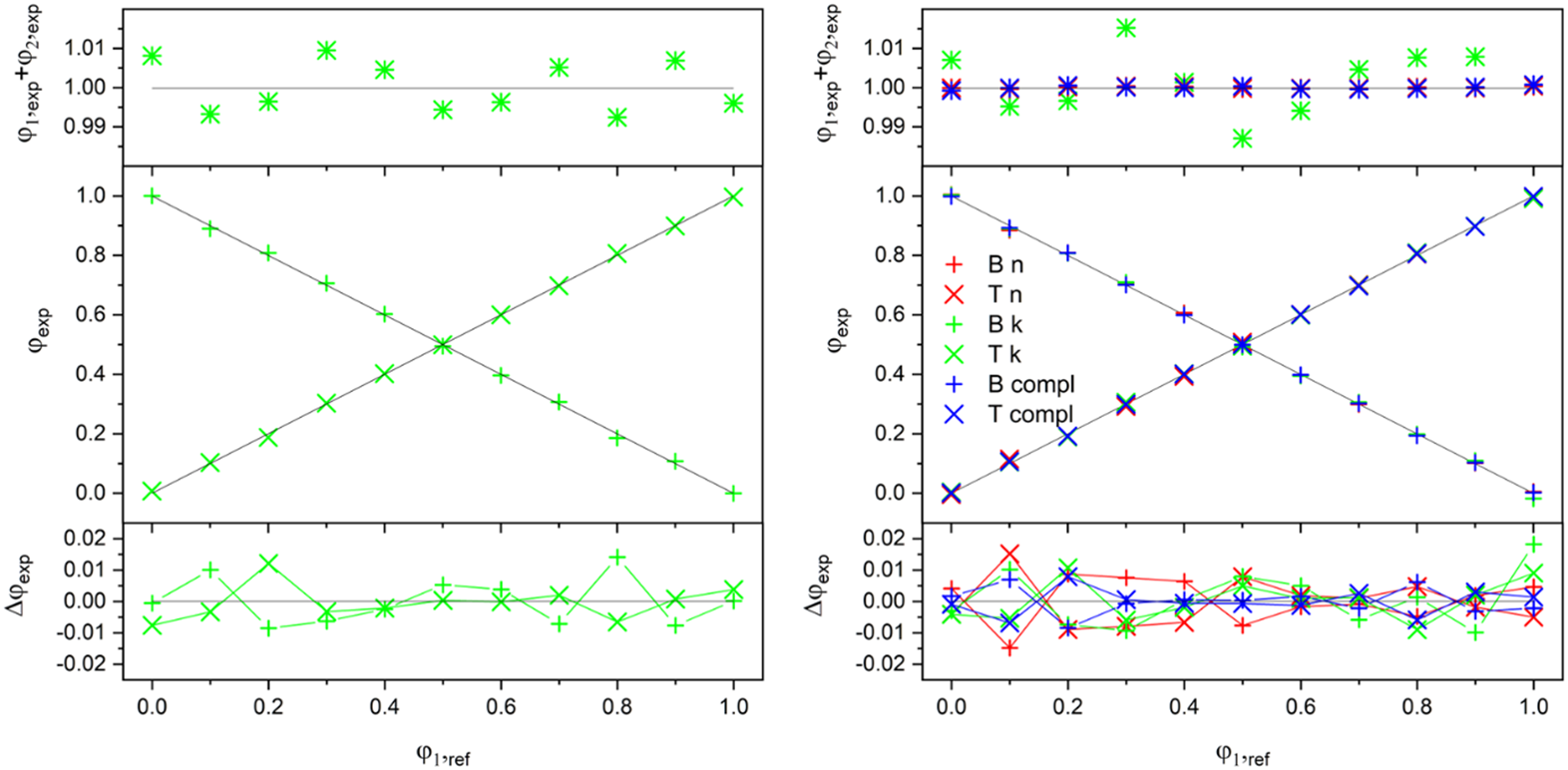
Top panels: Sum of the determined volume fractions. Center panels: Determined volume fractions (exp) versus actual volume fractions (ref); φ₁ represents the volume fraction of toluene. Bottom panels: Errors of the determined volume fractions. Left column: Volume fraction determination for uncorrected absorbance spectra. Right column: Results based on n- and k-spectra as well as $\hat{n}$ -spectra (compl) of benzene (B) and toluene (T) without error correction.

In contrast, for the benzene–cyclohexane system, ILS on uncorrected absorbance spectra, shown in Figure 3 alongside the refractive and absorption index spectra, performs less favorably, yielding a MAE of 0.0093 (Table II). In this system, it is advantageous to use only three wavenumber points, namely 674.5, 1479.5, and 2852 cm^–1, which are also indicated in Figure 3 (the raw spectra as well as the n- and k-spectra are provided as supporting information).

Figure 3.

Selected wavenumber ranges of the ATR, n- and k-spectra of the system benzene–cyclohexane. The wavenumber points chosen for ILS are indicated by vertical lines.

A key distinction in the benzene–cyclohexane system is the significant difference in n_∞ values, unlike in the benzene–toluene system. While n_∞ for benzene is 1.477, it is only 1.415 for cyclohexane.²⁸ The n_∞ values for the mixtures were calculated assuming the Lorentz–Lorenz relation holds (cf. Eq. 1). Therefore, we present these results with caution and recommend determining n_∞ experimentally in future studies, either through direct refractive index measurements or via external or internal reflection measurements below the critical angle.²⁰

The corresponding volume fractions are shown in the left panel of Figure 4, while those determined using the real, imaginary, and complex refractive index spectra are depicted in the right panel. When the absorption index spectra are used for ILS, the MAE is reduced to 0.0046, roughly half the value obtained using uncorrected absorbance spectra (Table II).

Figure 4.

Top panels: Sum of the determined volume fractions. Center panels: Determined volume fractions (exp) versus actual volume fractions (ref); φ₁ represents the volume fraction of cyclohexane. Bottom panels: Errors of the determined volume fractions. Left column: Volume fraction determination for uncorrected absorbance spectra. Right column: Results based on n- and k-spectra as well as $\hat{n}$ -spectra (compl) of benzene (B) and cyclohexane (C) without self-correction.

By contrast, when performing ILS on n-spectra with the same wavenumber points, the MAE value reaches an extremely high 0.1159. This outcome is unsurprising, as the changes in the refractive index function with respect to volume fraction are minimal at two of the three selected wavenumber points. In other words, at 674.5 and 2852 cm⁻¹, the refractive indices are nearly identical for all mixtures, see Figure 3 and Figure S3. As a consequence, the corresponding results are not displayed in Figure 4. Instead, we recalculated the MAE after redshifting all peaks by 1 cm⁻¹, which reduced the MAE from 0.1159 to 0.0089 (see Figure S3; using two points with slightly higher wavenumbers than 674.5 and 2852 cm⁻¹ would similarly improve the MAE). While identifying the optimal wavenumber points for ILS employing the refractive index function is challenging, it is relatively easy to obtain MAE values of 0.005 and below by selecting alternative points such as 650, 1400, 2150, and 2900 cm⁻¹ (this set was employed to obtain the MAE and the RSME shown in Table II) or 775, 1525, 2275, and 3025 cm⁻¹, among others (the MAE and RMSE values for all wavenumber sets discussed in this paragraph are provided in Table S2, Supplemental Material). This is possible due to the relatively large refractive index differences between the pure components, primarily stemming from differences in their n_∞ values. Therefore, also wavenumber points in the non-absorbing regions above 3100 cm^–1 can be selected for ILS using the n-spectra.

This improvement arises because, except at the peaks of the absorption index functions, changes in the refractive index function are proportional to the area of the absorption index bands. Thus, using the refractive index function is analogous to compressing the absorption index function or absorbance by integrating it across selected wavenumber regions, as was done in earlier approaches.³

In contrast, if the complex refractive index function is used for ILS, the same wavenumber points as those used for the absorption index function can be employed. In this case, the MAE is reduced from 0.0046 to 0.0025.

For CLS using all spectral points, the primary advantage of employing the complex refractive index function is indirect. Although the spectra of the pure components become complex-valued, the concentrations or volume fractions are still expected to remain real as already mentioned. However, due to systematic errors that introduce deviations from linearity (cf. Eq. 1), the resulting volume fractions also acquire a complex component. As we discovered, the imaginary part of these complex volume fractions reflects the underlying systematic errors. When multiplied by a scaling factor, determined by comparing the differences between determined and actual volume fractions in the calibration set for the “leave one out” scheme, the result closely resembles the actual volume fraction errors. In the absence of random (accidental) errors, this factor remains constant across volume fractions. Conversely, if systematic errors are absent, the factor behaves in a random, non-systematic way.

For the benzene–toluene system, the MAE could not be further reduced using the additional error correction mechanism introduced for complex-valued CLS, cf. Mayerhöfer et al.,²⁸ because ILS already removed the systematic error. However, in the benzene–cyclohexane system, a clear correlation remains between the experimental errors and the imaginary parts of the volume fractions determined by ILS (see the left panel of Figure 5). Applying this correlation using the additional correction mechanism allows for a reduction in the MAE from 0.0025 to 0.0019, although the improvement is less pronounced than with CLS (cf. Table II). This less pronounced improvement is also reflected in the fact that the factor shows some larger variance with the volume fraction (see Figure S2, Supplemental Material). Furthermore, for certain volume fractions, the errors actually increase (see the right panel of Figure 5). This is unsurprising given that the initial errors are already comparatively small.

Figure 5.

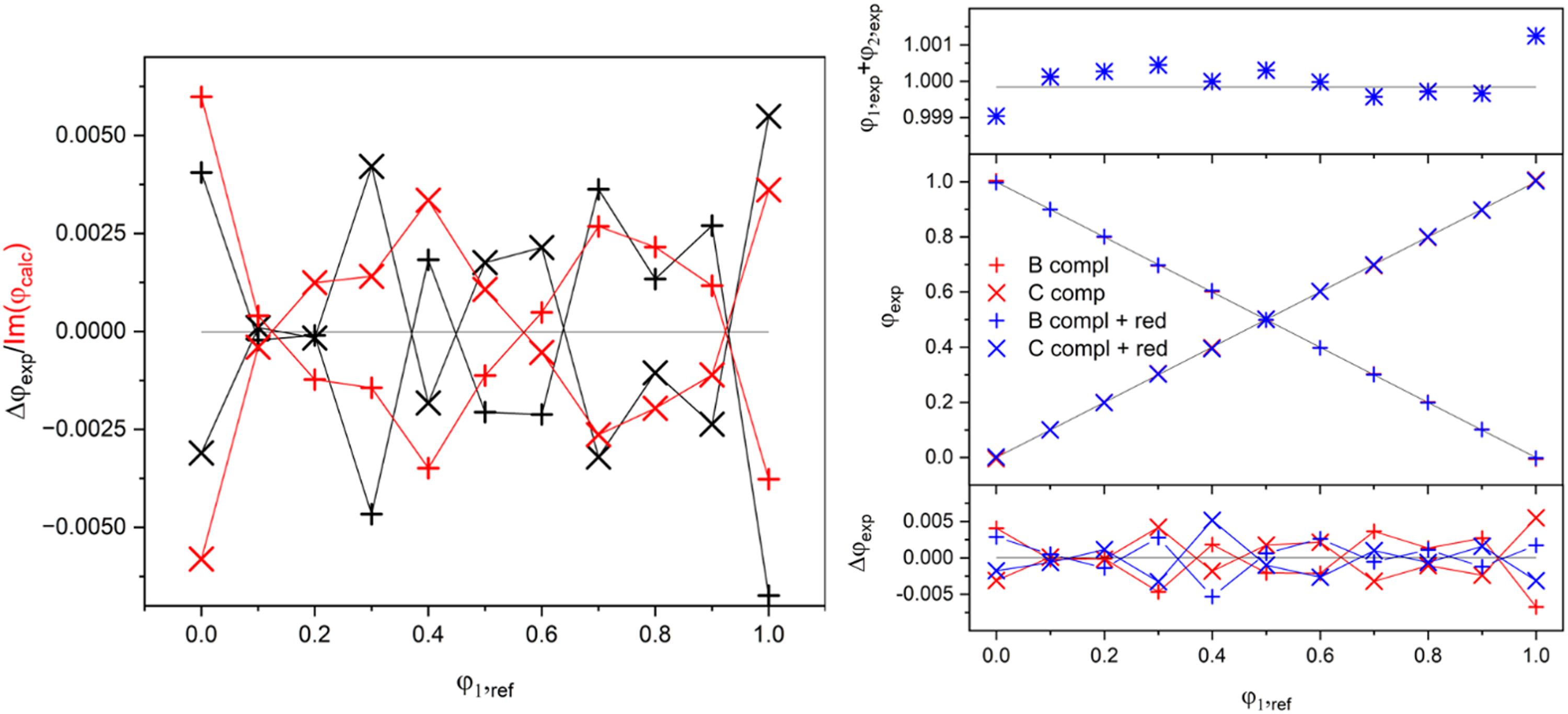
Left panel: Im(φ_exp) has been multiplied with a single factor so that the differences between Im(φ_exp) and Δφ_exp are minimized. Right column: $\hat{n}$ -spectra without (in red) and with self-correction (in blue) for benzene (B) and cyclohexane (C). Top panel: Sum of the determined volume fractions. Center panel: Determined volume fractions (exp) versus actual volume fractions (ref); φ₁ represents the volume fraction of cyclohexane. Bottom panel: Errors of the determined volume fractions.

Nevertheless, we believe that even in ILS, where the complex refractive index function yields immediate benefits, it remains worthwhile to explore whether the additional correction mechanism can further reduce errors.

Finally, we aim to compare the performance of complex-valued ILS with that of PLS, the workhorse of spectroscopy. While we would like to offer a sneak preview of what complex-valued PLS might achieve, a key methodological challenge remains unresolved. Specifically, since the eigenvectors (or latent variables) in PLS are not constrained to lie along the real or imaginary axes, applying PLS directly to complex-valued spectra requires further mathematical development to determine the optimal solution. We are currently working on such an extension, but it falls outside the scope of this study.

Instead, we demonstrate what is possible when conventional PLS1 regression³⁴ is applied separately to the n- and k-spectra and compare these results with those of ILS for the benzene–toluene and benzene–cyclohexane systems, as shown in Figure 6 (the number of latent variables was selected using a leave-one-out cross-validation). In the benzene–toluene system, complex-valued ILS slightly outperforms conventional PLS based on k-spectra when the number of latent variables in PLS equals the number of wavenumber points used in ILS,. When PLS is applied to n-spectra, its performance is slightly worse than when based on k-spectra.

Figure 6.

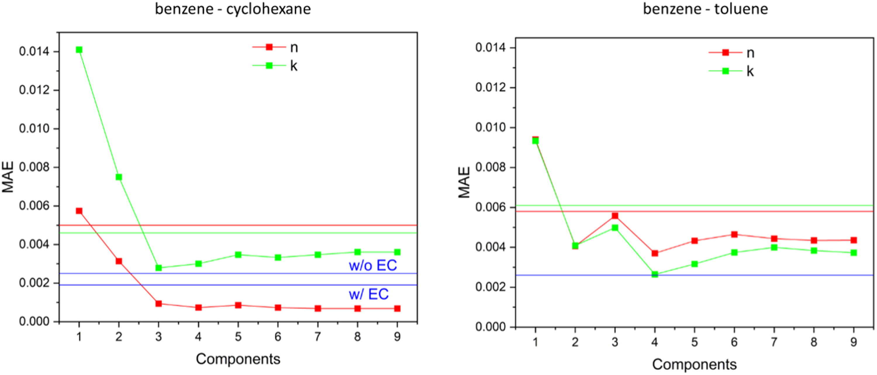
Comparison between the results of ILS regression represented by horizontal lines: n-spectra (red), k-spectra (green), and $\hat{n}$ -spectra (blue) and PLS1 regression in the system benzene–toluene and benzene–cyclohexane.

This trend reverses in the benzene–cyclohexane system: here, PLS based on n-spectra clearly outperforms PLS based on k-spectra, which is slightly surpassed by complex-valued ILS and clearly surpassed if an additional error correction was applied. The superior performance of n-spectra PLS in this case is due to the relatively large difference in the n_∞ values, as we will detail in an upcoming publication. There, we will also show that even in this favorable case, complex-valued PLS has the potential to push performance even further.

Conclusion

Employing complex-valued ILS regression in spectroscopy provides immediate benefits by significantly reducing errors compared to CLS regression. Unlike CLS, complex-valued ILS does not require an additional error reduction mechanism, although applying such a mechanism may further reduce errors in some cases, albeit less drastically and not universally.

Selecting the optimal wavenumber points for complex-valued ILS is simpler than for conventional ILS based on the absorption index function or absorbance. When the same wavenumber points are used, complex-valued ILS typically reduces errors by approximately 50%. Further error reduction can be achieved by avoiding points where the refractive index function remains unchanged and instead using points redshifted by 1 cm⁻¹.

Overall, for the systems studied, the performance of complex-valued ILS has been highly satisfactory. However, the extent of performance gains in more complex systems remains to be seen. Nevertheless, we believe that for systems with significant deviations from the Beer–Lambert approximation, complex-valued machine learning, and particularly complex-valued deep learning, could play a transformative role in the future.

Supplemental Material

sj-docx-1-asp-10.1177_00037028251358392 - Supplemental material for Complex-Valued Chemometrics in Spectroscopy: Inverse Least Squares Regression

Supplemental material, sj-docx-1-asp-10.1177_00037028251358392 for Complex-Valued Chemometrics in Spectroscopy: Inverse Least Squares Regression by Thomas G. Mayerhöfer, Oleksii Ilchenko, Andrii Kutsyk and Jürgen Popp in Applied Spectroscopy

Supplemental Material

sj-pdf-2-asp-10.1177_00037028251358392 - Supplemental material for Complex-Valued Chemometrics in Spectroscopy: Inverse Least Squares Regression

Supplemental material, sj-pdf-2-asp-10.1177_00037028251358392 for Complex-Valued Chemometrics in Spectroscopy: Inverse Least Squares Regression by Thomas G. Mayerhöfer, Oleksii Ilchenko, Andrii Kutsyk and Jürgen Popp in Applied Spectroscopy

Supplemental Material

sj-dat-3-asp-10.1177_00037028251358392 - Supplemental material for Complex-Valued Chemometrics in Spectroscopy: Inverse Least Squares Regression

Supplemental material, sj-dat-3-asp-10.1177_00037028251358392 for Complex-Valued Chemometrics in Spectroscopy: Inverse Least Squares Regression by Thomas G. Mayerhöfer, Oleksii Ilchenko, Andrii Kutsyk and Jürgen Popp in Applied Spectroscopy

Supplemental Material

sj-dat-4-asp-10.1177_00037028251358392 - Supplemental material for Complex-Valued Chemometrics in Spectroscopy: Inverse Least Squares Regression

Supplemental material, sj-dat-4-asp-10.1177_00037028251358392 for Complex-Valued Chemometrics in Spectroscopy: Inverse Least Squares Regression by Thomas G. Mayerhöfer, Oleksii Ilchenko, Andrii Kutsyk and Jürgen Popp in Applied Spectroscopy

Supplemental Material

sj-dat-5-asp-10.1177_00037028251358392 - Supplemental material for Complex-Valued Chemometrics in Spectroscopy: Inverse Least Squares Regression

Supplemental material, sj-dat-5-asp-10.1177_00037028251358392 for Complex-Valued Chemometrics in Spectroscopy: Inverse Least Squares Regression by Thomas G. Mayerhöfer, Oleksii Ilchenko, Andrii Kutsyk and Jürgen Popp in Applied Spectroscopy

Supplemental Material

sj-dat-6-asp-10.1177_00037028251358392 - Supplemental material for Complex-Valued Chemometrics in Spectroscopy: Inverse Least Squares Regression

Supplemental material, sj-dat-6-asp-10.1177_00037028251358392 for Complex-Valued Chemometrics in Spectroscopy: Inverse Least Squares Regression by Thomas G. Mayerhöfer, Oleksii Ilchenko, Andrii Kutsyk and Jürgen Popp in Applied Spectroscopy

Supplemental Material

sj-nb-7-asp-10.1177_00037028251358392 - Supplemental material for Complex-Valued Chemometrics in Spectroscopy: Inverse Least Squares Regression

Supplemental material, sj-nb-7-asp-10.1177_00037028251358392 for Complex-Valued Chemometrics in Spectroscopy: Inverse Least Squares Regression by Thomas G. Mayerhöfer, Oleksii Ilchenko, Andrii Kutsyk and Jürgen Popp in Applied Spectroscopy

Footnotes

Acknowledgments

Financial support from the EU, the “Thüringer Ministerium für Wirtschaft, Wissenschaft und Digitale Gesellschaft”, the “Thüringer Aufbaubank”, the Federal Ministry of Education and Research, Germany (BMBF), the German Science Foundation, the “Fonds der Chemischen Industrie” and the Carl-Zeiss Foundation is gratefully acknowledged.

Declaration of Conflicting Interests

The author(s) declared no potential conflicts of interest with respect to the research, authorship, and/or publication of this article.

Funding

The author(s) received no financial support for the research, authorship, and/or publication of this article.

ORCID iDs

Thomas G. Mayerhöfer

Jürgen Popp

Supplemental Material

All supplemental material mentioned in the text is available in the online version of the journal.

References

Wolberg

. Data Analysis Using the Method of Least Squares: Extracting the Most Information from Experiments. Berlin; Heidelberg: Springer, 2006.

Olivieri

. Introduction to Multivariate Calibration: A Practical Approach. Cham: Springer International Publishing, 2024.

Kramer

. Chemometric Techniques for Quantitative Analysis. Boca Raton, Florida: CRC Press, 1998.

Mayerhöfer

T.G.

Pahlow

Popp

. “The Bouguer–Beer–Lambert Law: Shining Light on the Obscure”. ChemPhysChem. 2020. 21(18): 2029–2046. https://doi.org/10.1002/cphc.202000464

Mayerhöfer

T.G.

. Wave Optics in Infrared Spectroscopy: Theory, Simulation, and Modeling. Philadelphia: Elsevier, 2024.

Mayerhöfer

T.G.

Ilchenko

Kutsyk

Popp

. “Beyond Beer’s Law: Quasi-Ideal Binary Liquid Mixtures”. Appl. Spectrosc. 2022. 76(1): 92–104. https://doi.org/10.1177/00037028211056293

Mayerhöfer

T.G.

Ilchenko

Kutsyk

Popp

. “Infrared Spectroscopy of Quasi-Ideal Binary Liquid Mixtures: The Challenges of Conventional Chemometric Regression”. Spectrochim. Acta, Part A. 2022. 280: 121518. https://doi.org/10.1016/j.saa.2022.121518

Mayerhöfer

T.G.

Dabrowska

Schwaighofer

Lendl

Popp

. “Beyond Beer's Law: Why the Index of Refraction Depends (Almost) Linearly on Concentration”. ChemPhysChem. 2020. 21(8): 707–711. https://doi.org/10.1002/cphc.202000018

Mayerhöfer

T.G.

Spange

. “Understanding Refractive Index Changes in Homologous Series of Unbranched Organic Compounds Based on Beer's Law”. ChemPhysChem. 2023. 24(19): e202300430. https://doi.org/10.1002/cphc.202300430

10.

Azzam

R.M.A.

Bashara

N.M.

. Ellipsometry and Polarized Light. Amsterdam: Elsevier, 1987.

11.

Bertie

J.E.

Eysel

H.H.

. “Infrared Intensities of Liquids I: Determination of Infrared Optical and Dielectric Constants by FT-IR Using the CIRCLE ATR Cell”. Appl. Spectrosc. 1985. 39(3): 392–401. https://doi.org/10.1366/0003702854248575

12.

Ohta

Ishida

. “Efficient Method for Optical Constant Determination by FTIR-ATR”. In: Heise

H.M.

Korte

E.H.

Siesler

H.W.

, editors. Proceedings SPIE 1575, 8th International Conference on Fourier Transform Spectroscopy. 1992. Pp. 604–605. https://doi.org/10.1117/12.56372

13.

Mayerhöfer

T.G.

Costa

W.D.P.

Popp

. “Sophisticated Attenuated Total Reflection Correction Within Seconds for Unpolarized Incident Light at 45°”. Appl. Spectrosc. 2024. 78(3): 321–328. https://doi.org/10.1177/00037028231219528

14.

Mayerhöfer

T.G.

Popp

. “Understanding Advanced Attenuated Total Reflection Correction: The Low Absorbance Assumption”. Appl. Spectrosc. 2024. 79(2): 298–305. https://doi.org/10.1177/00037028241268024

15.

Mayerhöfer

T.G.

Popp

. “Developing Correction Methods by Revisiting the Concept of Effective Thickness in Attenuated Total Reflection Spectroscopy”. Appl. Spectrosc. 2024. 79(3): 465–472. https://doi.org/10.1177/00037028241290838

16.

Mayerhöfer

T.G.

Popp

. “Understanding and Employing (Non-)Linearities in ATR Spectroscopy”. Appl. Spectrosc. 2024. https://doi.org/10.1177/00037028251317540

17.

Mayerhöfer

T.G.

Pahlow

Hübner

Popp

. “Removing Interference-Based Effects from the Infrared Transflectance Spectra of Thin Films on Metallic Substrates: A Fast and Wave Optics Conform Solution”. Analyst. 2018. 143(13): 3164–3175. https://doi.org/10.1039/C8AN00526E

18.

Mayerhöfer

T.G.

Pahlow

Hübner

Popp

. “Removing Interference-Based Effects from Infrared Spectra: Interference Fringes Re-Revisited”. Analyst. 2020. 145(9): 3385–3394. https://doi.org/10.1039/D0AN00062K

19.

Mayerhöfer

T.G.

Pahlow

Hübner

Popp

. “CaF₂: An Ideal Substrate Material for Infrared Spectroscopy?”. Anal. Chem. 2020. 92(13): 9024–9031. https://doi.org/10.1021/acs.analchem.0c01158

20.

Mayerhöfer

T.G.

Costa

W.D.P.

Popp

. “Combining Infrared Refraction and Attenuated Total Reflection Spectroscopy”. Appl. Spectrosc. 2024. 79(6): 1018–1027. https://doi.org/10.1177/00037028241283050

21.

Mayerhöfer

T.G.

Ivanovski

Popp

. “Infrared Refraction Spectroscopy: Kramers–Kronig Analysis Revisited”. Spectrochim. Acta, Part A. 2022. 270: 120799. https://doi.org/10.1016/j.saa.2021.120799

22.

Mayerhöfer

T.G.

Ivanovski

Popp

. “Infrared Refraction Spectroscopy”. Appl. Spectrosc. 2021. 75(12): 1526–1531. https://doi.org/10.1177/00037028211036761

23.

Dabrowska

Schwaighofer

Lendl

. “Mid-Infrared Dispersion Spectroscopy as a Tool for Monitoring Time-Resolved Chemical Reactions on the Examples of Enzyme Kinetics and Mutarotation of Sugars”. Appl. Spectrosc. 2024. 78(9): 982–992. https://doi.org/10.1177/00037028241258109

24.

Dabrowska

Lindner

Schwaighofer

Lendl

. “Mid-IR Dispersion Spectroscopy: A New Avenue for Liquid Phase Analysis”. Spectrochim. Acta, Part A. 2023. 286: 122014. https://doi.org/10.1016/j.saa.2022.122014

25.

Zorin

Gattinger

Ricchiuti

Lendl

, et al. “All-Mirror Wavefront Division Interferometer for Fourier Transform Spectrometry Across Multiple Spectral Ranges”. Opt. Express. 2025. 33(1): 867–884. https://doi.org/10.1364/OE.545267

26.

Pupeza

Huber

Trubetskov

Schweinberger

, et al. “Field-Resolved Infrared Spectroscopy of Biological Systems”. Nature. 2020. 577(7788): 52–59. https://doi.org/10.1038/s41586-019-1850-7

27.

Mayerhöfer

T.G.

Ilchenko

Kutsyk

Popp

. “Quantitative Chemometrics Using Refractive Index Spectra”. Appl. Spectrosc. 2025. https://doi.org/10.1177/00037028251345774

28.

Mayerhöfer

T.G.

Ilchenko

Kutsyk

Popp

. “Complex-Valued Chemometrics in Spectroscopy: Classical Least Squares Regression”. Appl. Spectrosc. 2025. https://doi.org/10.1177/00037028251343908

29.

Lorentz

H.A.

. Papers

Collected

. Volume II. Dordrecht: Springer-Science and Business Media, B.V., 1936.

30.

Lorentz

H.A.

. “Ueber die Beziehung zwischen der Fortpflanzungsgeschwindigkeit des Lichtes und der Körperdichte”. Annal. Physik. 1880. 245(4): 641–665. https://doi.org/10.1002/andp.18802450406

31.

Mayerhöfer

T.G.

Popp

. “Beyond Beer's Law: Revisiting the Lorentz–Lorenz Equation”. ChemPhysChem. 2020. 21(12): 1218–1223. https://doi.org/10.1002/cphc.202000301

32.

Mayerhöfer

T.G.

Popp

. “Beyond Beer's Law: Spectral Mixing Rules”. Appl. Spectrosc. 2020. 74(10): 1287–1294. https://doi.org/10.1177/0003702820942273

33.

Myers

T.L.

Tonkyn

R.G.

Danby

T.O.

Taubman

M.S.

, et al. “Accurate Measurement of the Optical Constants n and k for a Series of 57 Inorganic and Organic Liquids for Optical Modeling and Detection”. Appl. Spectrosc. 2018. 72(4): 535–550. https://doi.org/10.1177/0003702817742848

34.

Haaland

D.M.

Thomas

E.V.

. “Partial Least-Squares Methods for Spectral Analyses. 1. Relation to Other Quantitative Calibration Methods and the Extraction of Qualitative Information”. Anal. Chem. 1988. 60(11): 1193–1202. https://doi.org/10.1021/ac00162a020

Supplementary Material

Please find the following supplemental material available below.

For Open Access articles published under a Creative Commons License, all supplemental material carries the same license as the article it is associated with.

For non-Open Access articles published, all supplemental material carries a non-exclusive license, and permission requests for re-use of supplemental material or any part of supplemental material shall be sent directly to the copyright owner as specified in the copyright notice associated with the article.

0.00 MB

3.24 MB

0.99 MB

0.75 MB

0.49 MB

0.07 MB

0.08 MB