Data Adequacy Testing for Partial Least Squares Discriminant Analysis Using Raman Spectra

Abstract

Partial least squares discriminant analysis (PLS-DA) is often used for data sets that consist of a large number of potential predictors but relatively few observations such that chance correlations between predictors and response can occur that lead to false conclusions. Hence, there is a need for data adequacy testing before model building but currently no such method exists. In this work we propose one where we used random permutations to destroy the correlation structure between predictor and response data. This produced normal distributions of chance correlation coefficients that were used to find correlation coefficients in the non-permuted data that differed significantly from chance occurrences. Based on these distributions, we defined two novel null hypotheses to control for when a true null hypothesis is incorrectly rejected and the other for when a false null hypothesis is not rejected. To counter false positive errors, the standard significance levels were adjusted with predictor-based Bonferroni corrections. To counter false negative errors, we compared the true and permuted correlation coefficients in distribution tails. The outcomes of the hypothesis tests then indicated whether or not PLS-DA models could be successfully built from these data sets. We also investigated how to determine the number of samples needed for a data set with a given number of predictors. Simulations showed that our method produced significantly fewer false positives than PLS-DA (P = 0.0018, our method error rate 12 × less than PLS-DA error rate) but significantly more false negatives (P = 0.0003, our method error rate 4.5 × more than PLS-DA error rate). Data from Raman spectroscopy showed that the method transferred to real data. By pre-screening such data, our method can aid in assessing whether to proceed with model building and, when there is a need to increase the sample size, we show by how much.

Graphical abstract

This is a visual representation of the abstract.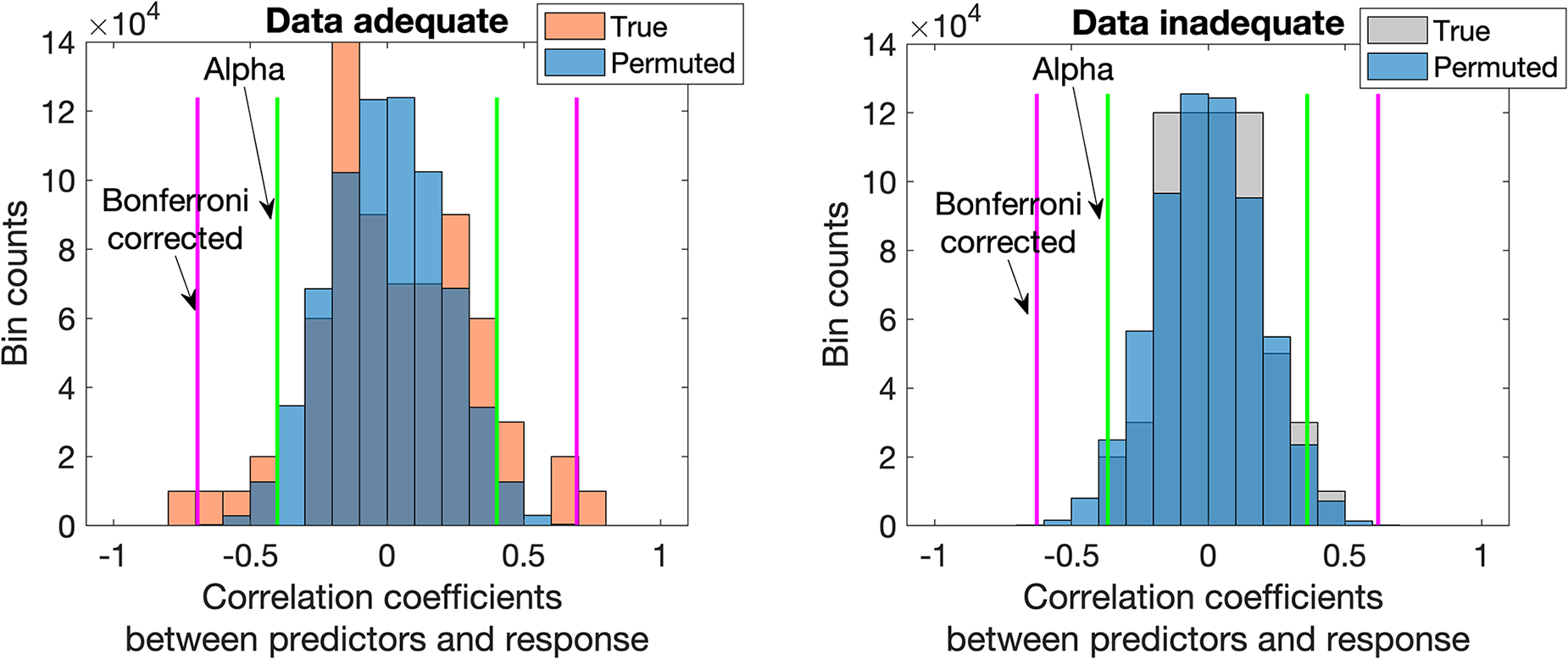

Keywords

Partial least squares discriminant analysis PLS-DA data adequacy testing permutation testing Bonferroni correction samples per predictor Raman spectroscopy peak fitting Type I error Type II error

Introduction

Projections to latent structures transform data to reduce their dimensionality, thereby facilitating further analyses. Widely used methods include some artificial neural networks (ANNs),¹ principal component analysis (PCA),² and partial least squares (PLS)³ methods. PLS methods are used in numerous fields including economics,³ chemometrics,^4,5 spectroscopy,^6–10 neuroimaging and behavior,^11,12 and metabolomics and biomedicine.^13–15 Partial least squares regression is a regression method that aims to extract information from an observational set of independent variables or predictors to predict one or more continuous dependent variables or responses.¹¹ When the responses are categorical, this is partial least squares discriminant analysis (PLS-DA).^5,16 In PLS-DA the predictors are linearly combined into latent variables (LVs) to discriminate between categories. In essence, an observational data matrix X of predictors is modeled in a PCA-like manner as scores T and weights W (from which loadings P are derived). Likewise, the response matrix Y is modeled as scores U and loadings C. Importantly, the modeling of X and Y occurs simultaneously subject to maximizing the covariance between T and U and deflating X and Y after the extraction of every LV.^5,17 Thus, unlike unsupervised PCA, the LVs are chosen to maximize the covariance between the scores of X and Y. Therefore, the first LVs covary as much as possible with Y. Thus, they are the LVs extracted from X most able to predict Y.¹³ The process starts with calculating the initial vector of weights as¹⁷

w = X^{'} \cdot y

(1)

where X is a n × p matrix of n observations each with p predictors, the prime indicates a transpose and y is a n × 1 response vector. Thus, w is a p × 1 vector that consists of dot products w between all p predictors of dimension n × 1 and the response y where the dot product between any predictor x′ and y is given as

\begin{aligned} x^{'} \cdot y = ‖ x^{'} ‖ ‖ y ‖ \cos θ \\ w = ‖ x^{'} ‖ ‖ y ‖ \cos θ \end{aligned}

(2)

The correlation coefficient r is defined for two k × 1 vectors a and b as

\begin{aligned} r = a^{'} \cdot b / ‖ a^{'} ‖ ‖ b ‖ \\ = \cos θ \end{aligned}

(3)

and can be replaced in Eq. 2 to yield

w = ‖ x^{'} ‖ ‖ y ‖ r

(4)

Thus, the initial weights are related to the correlation coefficients between predictors and response. We exploit this relationship between weights and correlation coefficients as will be detailed further below.

Benefits of PLS-DA arise from its ability to accommodate noisy and missing variables.⁵ Compared with multiple linear regression, PLS-DA is also less vulnerable to collinearities in the observational data set that render impossible or unstable the inversion of X needed to obtain the multiple linear regression coefficients.^5,13 Furthermore, PLS-DA loadings principally point more in the direction of greatest separation between classes rather than in the direction of greatest dispersion of data by PCA.¹⁸ Hence, it reveals more information about how the predictors relate to the response, and this can be further enhanced with orthogonal PLS-DA.¹³ PLS-DA is also particularly well suited to deal with few observations of large to very large numbers of independent variables.¹³ Such situations occur, for example, in chromatographic,¹⁹ metabolomic,¹⁵ brain behavior,^20,21 and vibrational spectroscopy analyses.²² These advantages have led to the considerable popularity of PLS-DA,^11,16,23,24 yet concerns remain about the accuracy and stability of PLS-DA models.^{12,14,17,20,25} Specifically, about increases in the probability that a predictor could be found to correlate with a response by chance in cases with few observations and many more predictors.^12,17,20 This results in models that might excellently fit the data, but are fundamentally flawed as they arise from coincidence.^12,14

Two classes of remedies have been developed to deal with this difficulty. The first emphasizes the need for much larger sample sizes than commonly used to avoid overfitting and to obtain accurate and stable models.^12,20 For example, from a nearly linear relationship found between the number of predictors and model quality, it has been deduced that “about 50” observations per predictor are needed to obtain a good quality model for a between-set correlation of 0.3 for canonical correlation analysis; somewhat more for PLS.¹² This implies that either large numbers of observations must be pursued for relatively smaller effect sizes or large effect sizes must be pursued when only small sample sizes are available.^26–29 The second class of remedies involves efforts to improve the quality of model building and assess the reliability of models based on the limited numbers of available observations,^21,28,29 often when the difficulty and costs of obtaining large numbers of observations are prohibitive.^13,17,20 Cross-validation (CV) schemes are meant to improve model building and model selection and avoid obtaining unreliable models. With internal validation schemes, all available samples are used whereas with external validation either new samples are needed or a portion of the available samples are set aside for a single use test of the selected model.^14,30,31 In permutation tests, the response is extensively randomly permuted to see if a model can correctly classify these now incorrect responses. For an accurate model, this should not be possible because the correlation structure of the data sets would have been destroyed.^17,30 Associated with model building and validation schemes are various quality assessment methods such as classification rate,¹⁴ area under the receiver operating characteristic,³² Q² and discriminant Q²,³³ root means square (RMS) errors of prediction³¹ and R² values.¹³ However, problems also exist with some of these metrics. A poor model could produce good R² and RMS figures of merit.³¹ A poor model could also produce a large Q².¹³ Furthermore, it is unknown which values of these metrics are indicative of a good model.³⁰ Overall, the classification rate (CR) and area under the receiver operating characteristic curve (AUC) have been recommended as superior diagnostic statistics compared to Q² and discriminant Q².³²

When confronted with the common circumstances of restricted sample sizes, the first class of remedies is not available. However, neither can the remedies of the second class be used. This is because a correlation might still occur by chance between large numbers of predictors and one or more responses.^12,17,31 From the very first step where the initial weights are calculated (i.e., Eq. 1), chance correlations in a given data set might then be incorporated into LVs and thereby compromise the model. These chance correlations will also persist regardless of how the sample is partitioned for CV. Furthermore, they persist when permutations are applied because the permutations are applied to models based on data already containing chance correlations and cannot address the presence of these chance correlations. In other words, though models based on true response data cannot predict permuted response data very well, the model results obtained from the true response data, even if significantly different from the distribution of model results based on permuted responses,³⁰ would still be based on one or more chance correlations already present in the true response data. The conclusion then drawn is that the predictor data contained information about the response data when that was not true. This leads to a situation akin to a Type I error where the data null hypothesis (the predictor and response data have inadequate correlation coefficients) is rejected when it should not be rejected.

Our work was motivated by the insufficiency of current remedies to address the problem of chance correlations in the data. Furthermore, we intended to focus directly on the suitability of a given data set for PLS-DA use because at the origin of these problems are the data itself. Thus, we present here a method to define and test a data hypothesis while controlling for the Type I error. This is followed by a method to reduce the likelihood of then making a Type II error where the experimental hypothesis is rejected when it should not be (the predictor and response data do have adequate correlation coefficients). In a two-stage approach, we first apply a Bonferroni correction³⁴ to the standard significance level (α = 0.05) through division by the number of predictors in the data set to counter Type I errors. In ambiguous cases, to counter making Type II errors, we proceed to a second stage where we compare the correlation coefficients between predictors and permuted response data with those between predictors and true response data for all correlation coefficients that exceed the standard significance level. We do not eliminate individual predictors and thus do not impede the synergy that they collectively might exhibit, but we assess whether the data set as a whole might be used successfully. Importantly, in contrast to the more common use of permutation tests to evaluate model performance, we do not directly address the matter of model building but instead address the suitability of the data for building a model.

This work is structured as follows. In the Introduction we outline a currently widely acknowledged and significant problem with PLS-DA, how this motivated our work and the approach we took. In the Methods section, we describe the synthetic and real data used, how the hypothesis tests were defined and implemented, the corresponding PLS-DA models used for comparisons with our method and information about data analyses. In the Results section, we report and discuss the comparative outcomes for the synthetic and real data. Further discussions of the proposed method, including estimating the number of observations needed and the method’s limitations, follow in the Discussion section. Finally, conclusions drawn from the results are presented.

Methods

Predictors and Response

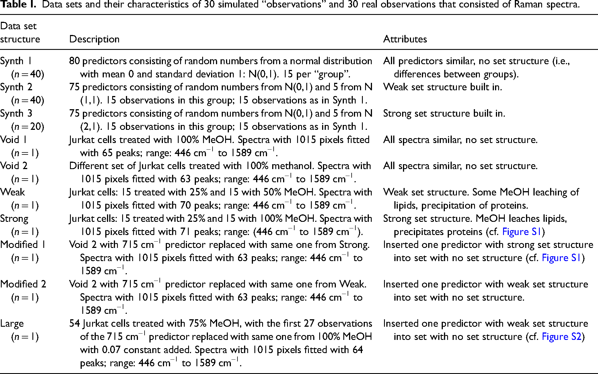
We created three synthetic data sets (Synth 1, Synth 2, and Synth 3) with no, weak, and strong structures respectively, to evaluate the method against known outcomes. We replicated these sets to establish estimates of false positive and false negative rates for our hypothesis tests. The number of replicates used and their attributes are listed in Table I. The response consisted of a single 30-element column where the top 15 entries were coded as zeros and the remainder as ones. We further used six different sets of Raman microscopy spectra, also listed in Table I, to evaluate the method on real world data. Briefly, a confocal Raman microscope (inVia, Renishaw, UK) equipped with a 785 nm diode laser that provided ∼100 mW power at the sample and a 50× objective lens (Leica Microsystems, Germany) was used to collect 50 to 70 spectra of 10 s acquisition time per sample with each spectrum containing information from 10 to15 cells. These spectra were from cells treated with different concentrations of methanol (MeOH) to assess its effects as a fixative.³⁵ Depending on the concentration of MeOH used, the measured spectra differ.³⁵ For example, MeOH caused a greater dissolution of lipids from Jurkat cells when treated with 100% MeOH compared to those treated with 25% MeOH, resulting in smaller areas of the 715 cm^–1 phosphatidylcholine peaks. More details about these spectra and methods can be found in Rangan et al.³⁵

Table I.

Data sets and their characteristics of 30 simulated “observations” and 30 real observations that consisted of Raman spectra.

Data set structure	Description	Attributes
Synth 1 (n = 40)	80 predictors consisting of random numbers from a normal distribution with mean 0 and standard deviation 1: N(0,1). 15 per “group”.	All predictors similar, no set structure (i.e., differences between groups).
Synth 2 (n = 40)	75 predictors consisting of random numbers from N(0,1) and 5 from N(1,1). 15 observations in this group; 15 observations as in Synth 1.	Weak set structure built in.
Synth 3 (n = 20)	75 predictors consisting of random numbers from N(0,1) and 5 from N(2,1). 15 observations in this group; 15 observations as in Synth 1.	Strong set structure built in.
Void 1 (n = 1)	Jurkat cells treated with 100% MeOH. Spectra with 1015 pixels fitted with 65 peaks; range: 446 cm^–1 to 1589 cm^–1.	All spectra similar, no set structure.
Void 2 (n = 1)	Different set of Jurkat cells treated with 100% methanol. Spectra with 1015 pixels fitted with 63 peaks; range: 446 cm^–1 to 1589 cm^–1.	All spectra similar, no set structure.
Weak (n = 1)	Jurkat cells: 15 treated with 25% and 15 with 50% MeOH. Spectra with 1015 pixels fitted with 70 peaks; range: 446 cm^–1 to 1589 cm^–1.	Weak set structure. Some MeOH leaching of lipids, precipitation of proteins.
Strong (n = 1)	Jurkat cells: 15 treated with 25% and 15 with 100% MeOH. Spectra with 1015 pixels fitted with 71 peaks; range: (446 cm^–1 to 1589 cm^–1).	Strong set structure. MeOH leaches lipids, precipitates proteins (cf. Figure S1)
Modified 1 (n = 1)	Void 2 with 715 cm^–1 predictor replaced with same one from Strong. Spectra with 1015 pixels fitted with 63 peaks; range: 446 cm^–1 to 1589 cm^–1.	Inserted one predictor with strong set structure into set with no set structure (cf. Figure S1)
Modified 2 (n = 1)	Void 2 with 715 cm^–1 predictor replaced with same one from Weak. Spectra with 1015 pixels fitted with 63 peaks; range: 446 cm^–1 to 1589 cm^–1.	Inserted one predictor with weak set structure into set with no set structure.
Large (n = 1)	54 Jurkat cells treated with 75% MeOH, with the first 27 observations of the 715 cm^–1 predictor replaced with same one from 100% MeOH with 0.07 constant added. Spectra with 1015 pixels fitted with 64 peaks; range: 446 cm^–1 to 1589 cm^–1.	Inserted one predictor with weak set structure into set with no set structure (cf. Figure S2)

The spectra were preprocessed in sequence, correcting the baseline with 15 iterations, removing artefacts, and smoothing with a peak fitting method, with automated algorithms published elsewhere³⁶ and then averaged. The peaks of the averages were fitted with a moving window Gaussian peak fitting method and parameter settings also fully detailed elsewhere.³⁷ An example is shown in Figure 1. Peak fit parameters were used to normalize peak areas to that of the 782 cm^–1 composite nucleic acid peak area and the normalized peak areas constituted the set of predictors. Using peak fit parameters reduced each spectrum of 1015 wavenumber predictors, many of them highly collinear, to approximately 65 predictors with reduced collinearity (cf. Table I). However, reduced collinearities remain due to the presence of different Raman bands belonging to the same molecule. The response consisted of a single 30-element column where the top 15 entries were coded as ones and the remainder as zeros.

Figure 1.

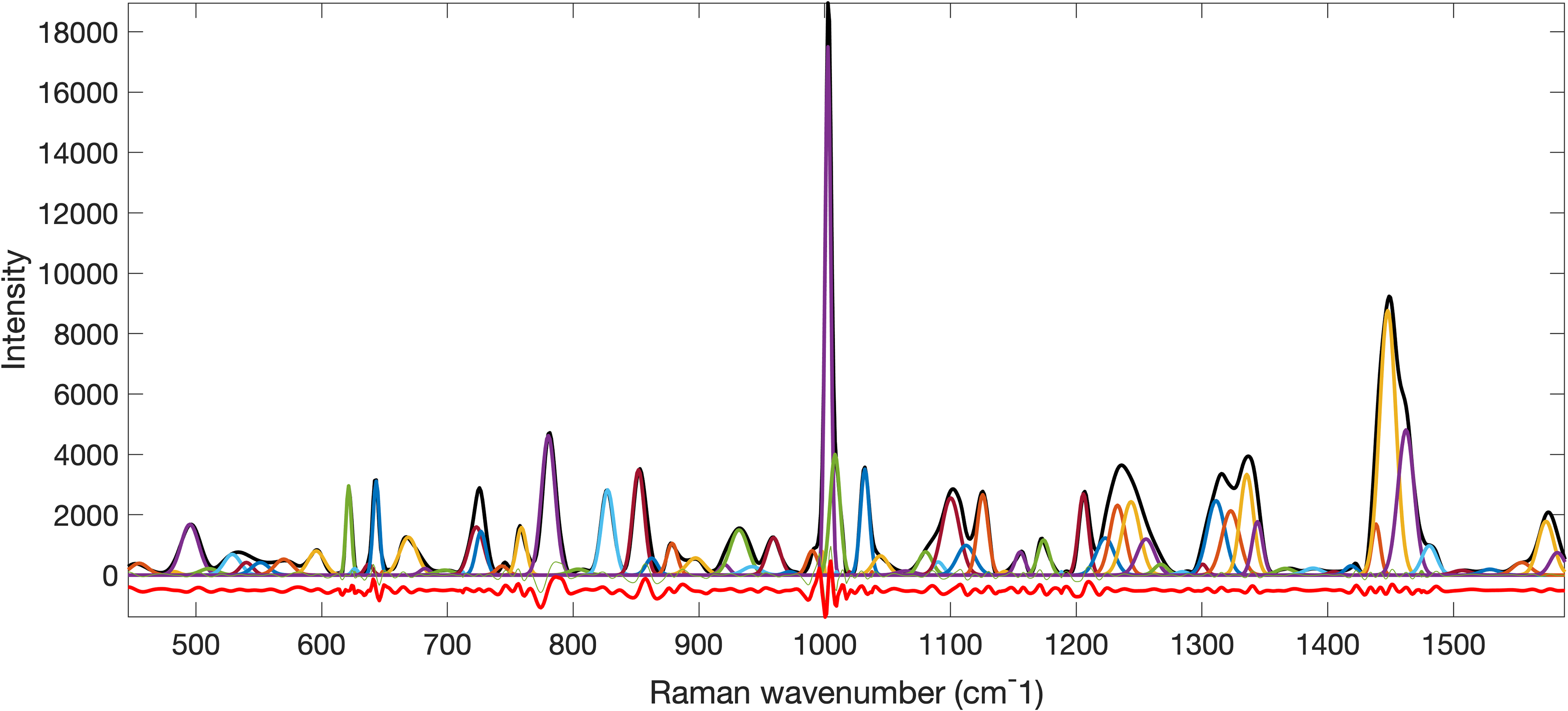
An example preprocessed spectrum shown as a black trace with individually fitted peaks superimposed thereon in various colors. The residual is shown as a negatively offset red trace.

Hypothesis Testing

We defined a general data adequacy null hypothesis as one where the predictors and response have no relationship. Specifically, that there are no correlation coefficients between the predictors and the response that exceed the critical correlation coefficient values. The critical values were established from correlation coefficients between the predictors and the permuted response as described next.

For every data set, we created 10 000 random permutations by selecting randomly 15 elements from the 30 elements of the response and flipping their group assignments. Thus, after every permutation exactly half of the response variable was coded incorrectly. We then determined the correlation coefficients between the predictors and the permuted response. These correlation coefficients produced near normal distributions (more in the Discussion section) that were fitted with true normal distributions from which we determined critical values for the correlation coefficients to perform significance tests. These critical values pertained to the standard α = 0.05 and the Bonferroni corrected α = 0.05/(number of predictors). The primary null hypothesis (H_0B) was rejected when one or more correlation coefficients between the predictor variables and the true response variable exceeded the Bonferroni corrected critical values on either side of the fitted distribution (negative correlations have as much predictive power as positive ones).

We also performed a secondary hypothesis test to establish if a significant difference existed between two medians: the median of absolute correlation coefficients between the true response and the predictors (true condition) and the median of absolute correlation coefficients between the response permutations and the predictors (permutation condition). This last test of the null hypothesis (H_0W) was based on a Wilcoxon rank sum test where, for both groups, only correlation coefficients that exceeded the α = 0.05 critical values were used. The rationale for this was that an adequate data set might yet have heavier tails than an inadequate data set even though no predictor in that first set might meet the Bonferroni criterion. A rank sum test was used because few correlation coefficients of the true condition might exceed the critical values for α = 0.05, thus violating the assumption of normality required for parametric tests. These correlation coefficients, in both conditions, are also not normally distributed. The H_0W is rejected when the correlation coefficient median of the true condition exceeds the correlation coefficient median of the permutation condition in a region where the correlation coefficients might still determine successful modeling. The secondary test was intended to resolve ambiguous cases where high absolute correlation coefficients did not exist between predictor and response data, but lower absolute correlation coefficients did exist that might permit modeling. Though we advise against modeling when the H_0W is not rejected, its outcome might still serve as a Bayesian prior to resolve subsequent uncertain modeling outcomes.

PLS-DA Modeling

After testing all nine data sets, we used PLS-DA to compare the results with those predicted from the hypothesis tests.

Because there is a certain lack of consensus on what constitutes a good model,³⁰ we considered more than just one model. For the synthetic data, we considered two models to bracket the number of LVs used. The first model found the minimum number of LVs needed to produce the minimum number of misclassifications (NMCs) and the second used that number of LVs that resulted in the minimum prediction error sum of squares (PRESS). For the real data, because there were fewer data sets, we could use a more nuanced approach. Where “good” (i.e., adequate) data produced models with no classification errors based on the minimum PRESS, we also considered more parsimonious models. These were based on non-significant as well as significant van der Voet T² differences between the model with fewer LVs and the minimum PRESS model²⁴ provided the parsimonious one still produced no classification errors. Where “poor” (i.e., inadequate) data produced models with classification errors based on the minimum PRESS, we also considered one or more less parsimonious models based on non-significant van der Voet T² differences to confirm that a still reasonably parsimonious model could not be built with the given data set. The data were centered, scaled, and standardized using options available in the below used software package. We used leave-one-out cross-validation, as it produces the most optimistic models¹⁴ and so would constitute the most conservative tests of data adequacy. If a model could not be built using the most optimistic approach, it is not likely to be built with a more stringent approach.

Data Analysis

Data analyses were performed using Matlab R2017b and R2023b (The MathWorks Inc., USA) using built-in and custom written code. PLS-DA modeling used JMP Student Edition v.18.2.2 (JMP Statistical Discovery LLC., USA).

Results

Histograms of non-permuted (“true”) and permuted data are shown in Figure 2 (left panel). In the right panel, the 10 000 random permutations of the response data, which generated a nearly normal correlation coefficient distribution. We observed this for all data sets as also shown in Figures 3 through 6. The normal distributions were used to determine the critical correlation coefficients for every set, with each distribution tail containing 2.5% of the total area under the fitted curve, thus consistent with the standard α = 0.05 significance level. The Bonferroni corrected α was determined from division of α by the number of predictors or peaks in the respective data sets. The critical correlation coefficients for these two significance levels are shown as green and magenta lines, respectively, in the figures.

Figure 2.

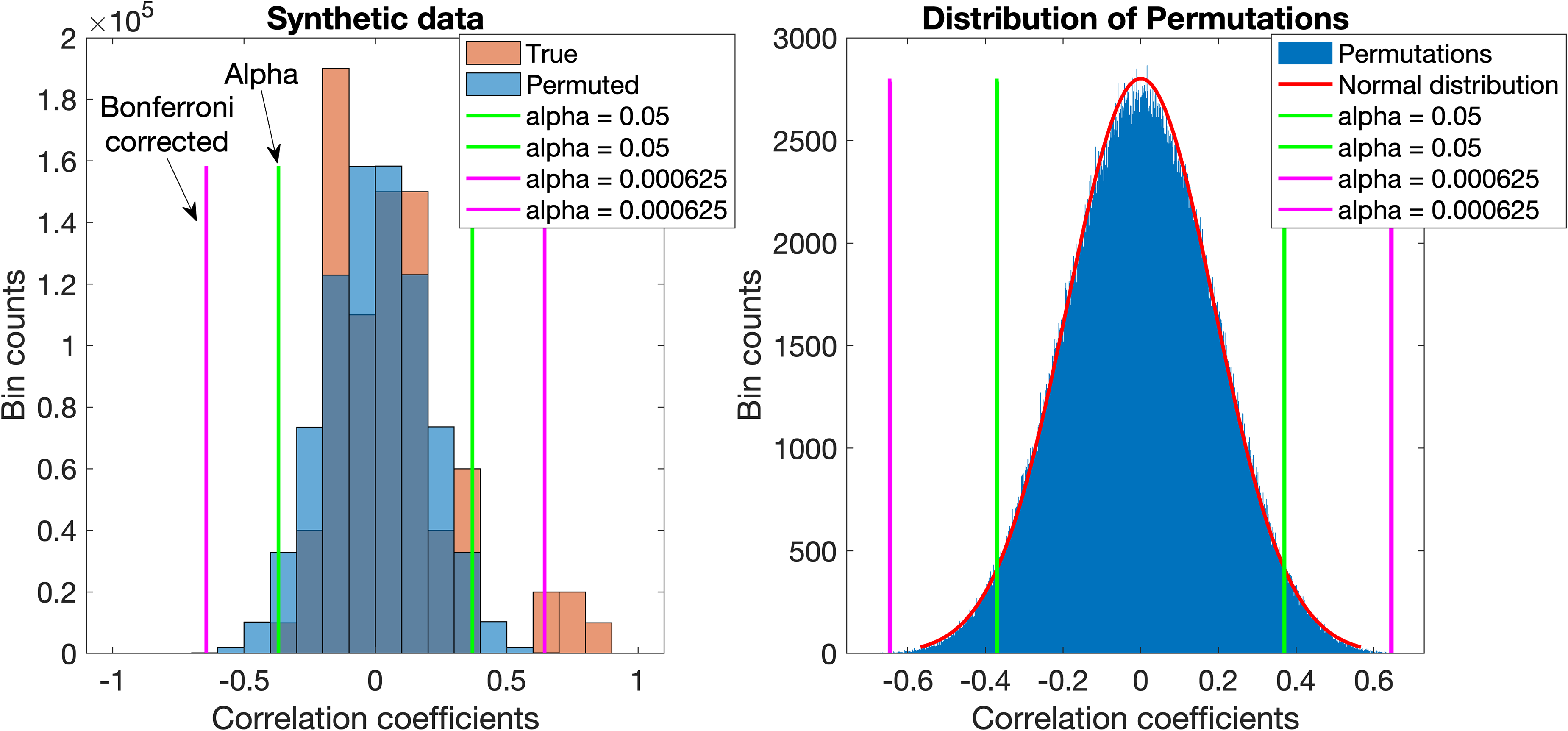
Histograms of correlation coefficients between predictor and true response data (orange) and between predictor and permuted response data (blue) are shown in the left panel. Where distributions overlap, the color is darker. The nearly normal distribution of the permutations’ correlation coefficients with a superimposed fitted normal curve is shown in the right panel. Critical correlation coefficients for standard and Bonferroni corrected significance levels determined from the fits are shown as green and magenta lines, respectively.

Figure 3.

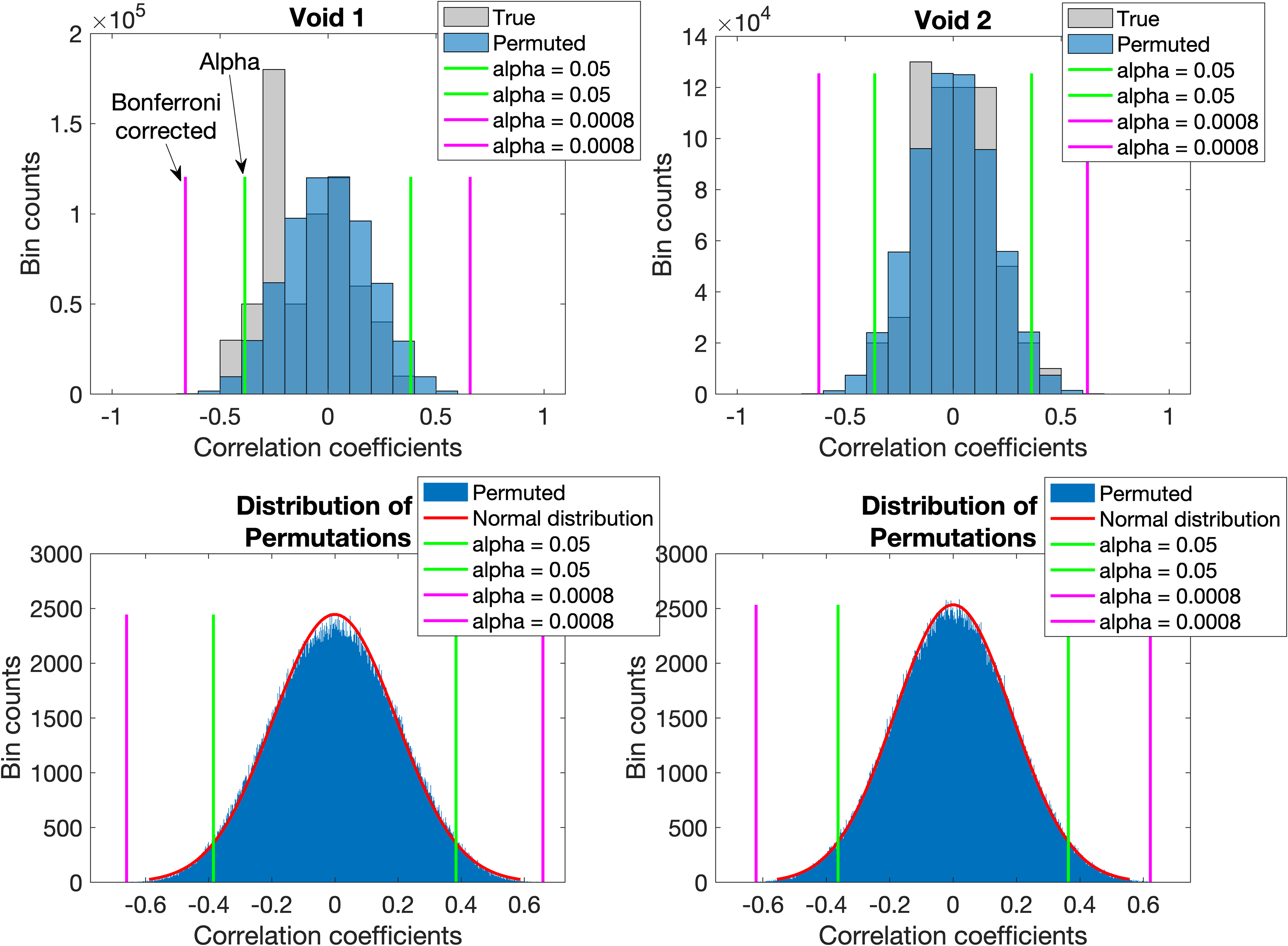
For replicate data with void predictor structure, histograms of correlation coefficients between predictor and true response data (coded grey to indicate void structure) and between predictor and permuted response data (blue) are shown in the top panels. Where distributions overlap, the color is darker. The distribution of the permutations’ correlation coefficients with normal probability distribution fits are in the respective bottom panels. Critical correlation coefficients for standard and Bonferroni corrected significance levels determined from the fits are shown as green and magenta lines, respectively. For both sets, it is evident that the correlation coefficients between predictor and true response data did not exceed the critical values for the Bonferroni corrected α. Thus, in both cases the H_0B was not rejected. Neither did the median absolute correlation coefficients between predictor and true response data exceed those between predictor and permuted response data in the regions beyond the green lines. Thus, in both cases the H_0W was also not rejected and the data were considered inappropriate for PLS-DA.

For the synthetic data, we found that, in the case of Synth 1, our method produced one false positive data set out of 40 trials. PLS-DA models built with the same data resulted in 12 false positive models. This was a statistically significant difference in classification accuracy (Matlab testcholdout P = 0.0018, our method error rate = 0.0250, PLS-DA error rate = 0.3000). In the case of Synth 2, there were 18 false negatives with our method but only four produced by the PLS-DA models. This difference was also statistically significant (testcholdout P = 0.0003, our method error rate = 0.4500, PLS-DA error rate = 0.100). In the Synth 3 case, neither approach produced false negatives. The outcomes of these tests are reported in Table S1 (Supplemental Material).

We next consider the results of the real data sets. Table II summarizes the outcomes of the hypothesis tests. Detailed statistics (h, P, z, rank sum, medians) of the Wilcoxon tests can be found in Table S2 of the Supplemental Material.

Table II.

Hypothesis tests of data adequacy for PLS-DA modeling for six real data sets with various characteristics (cf. Table I). Also shown are the number of correlation coefficients that exceed the critical values of the standard and Bonferroni corrected significance levels.

Data set structure	α	Number in excess	Bonferroniα	Number in excess	H_0B	H_0W	Outcome of hypothesis tests
Void 1	0.05	5	α = 0.05/65	0	0	0	Data inadequate
Void 2	0.05	2	α = 0.05/63	0	0	0	Data inadequate
Weak	0.05	11	α = 0.05/70	2	1	1	Data adequate
Strong	0.05	53	α = 0.05/71	33	1	1	Data adequate
Modified 1	0.05	3	α = 0.05/63	1	1	0	Data adequate
Modified 2	0.05	2	α = 0.05/63	0	0	0	Data inadequate
Large	NA	NA	NA	NA	NA	NA	NA

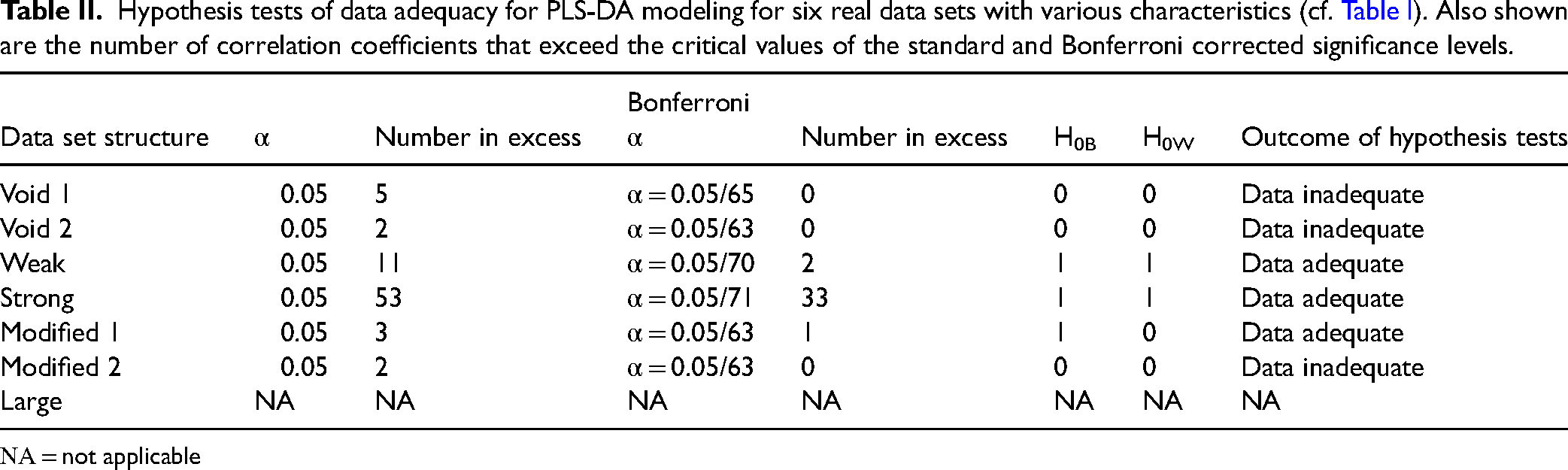
ΝΑ = not applicable

The correlation coefficient distributions of permuted and true response data are shown in Figure 3 for the Void 1 and Void 2 sets. Data histograms are shown in the top panels and, in the respective bottom panels, the distribution of generated correlation coefficients with normal probability distribution fits. For both sets, it is evident that the correlation coefficients between predictor and true data (grey bars) did not exceed the critical values for the Bonferroni corrected α. Thus, in both cases the H_0B was not rejected. However, 5 and 2 (see Table II) correlation coefficients did exceed the standard α values. In the case of Void 1, the median absolute true condition correlation coefficient was 0.4231, less than the 0.4301 of the median absolute permutation condition correlation coefficient where these were calculated only for absolute correlation coefficients exceeding the standard alpha. Thus, the H_0W (P = 0.8650) was also not rejected. For Void 2, a similar result for H_0W (P = 0.7078) was observed with respective median values of 0.3990 and 0.4120. Due to the failure to reject any of the null hypotheses, these data sets were considered not suitable for PLS-DA as would be expected for these sets.

For the Weak group structure data set, higher correlation coefficients were observed between predictor and true response data as expected. This is shown in the Figure 4 left panels (orange bars) where 11 coefficients exceeded the standard significance levels and two coefficients exceeded the Bonferroni corrected significance levels. This still led to a rejection of the H_0B and the data set was therefore considered appropriate for PLS-DA. The respective median correlation coefficients for the true and permutation conditions were 0.5758 and 0.4490 with rejection of H_0W (P = 0.0003).

Figure 4.

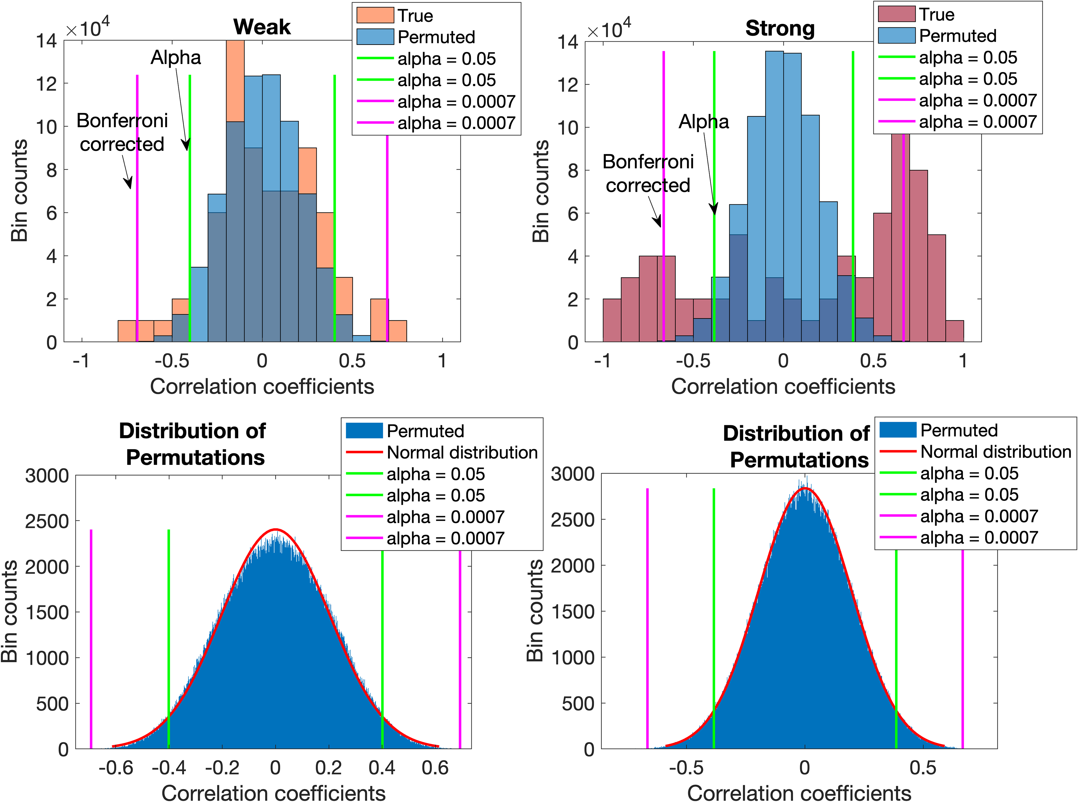
For data with weak predictor structure, histograms of correlation coefficients between predictor and true response data (coded orange to indicate weak structure) and between predictor and permuted response data (blue) are shown in the left panel. For data with strong predictor structure, the histograms of true (coded maroon to indicate strong structure) and permuted data (blue) are shown in the right panel. Where distributions overlap, the color is darker. The distributions of the permutations’ correlation coefficients with normal probability distribution fits are in the respective bottom panels. For both sets, it is evident that correlation coefficients between predictor and true response data exceeded the critical values for the Bonferroni corrected α. Thus, the H_0B was rejected and the data considered suitable for PLS-DA.

The highest correlation coefficients were observed between predictor and true response data for the Strong set shown in the Figure 4 right panels (maroon bars). The histogram shows that numerous correlation coefficients exceeded the critical values (53) for the standard α level (Table II). Numerous correlation coefficients also exceeded the critical values (33) for the Bonferroni corrected α (Table II). Thus, the H_0B was rejected and no need existed for the secondary hypothesis test. However, for the sake of completeness and contrast, we also performed the secondary test. The median absolute true condition correlation coefficient was 0.6852, substantially more than the 0.4348 of the median absolute permutation condition correlation coefficient where these were calculated as explained before. Thus, the H_0W (P < 0.0001) was also rejected. Though both hypothesis tests produced the same outcome, it was sufficient to conclude from the rejection of H_0B that this data set was suitable for PLS-DA.

To mimic the presence of a happenstance correlation between predictor and response data, the Void 2 set was modified by replacing a predictor with a low correlation coefficient with the response with a predictor from the Strong set that had a high correlation coefficient with the response to create the Modified 1 set (cf. Table I). This correlation coefficient was high enough to exceed the critical value of the Bonferroni corrected alpha level as shown in Figure 5 (left panels). It led to a rejection of the H_0B. Thus, the data was then considered suitable for PLS-DA even though the medians for the true and permutation conditions were 0.4058 and 0.4111, respectively, and the H_0W (P = 0.2805) was not rejected.

Figure 5.

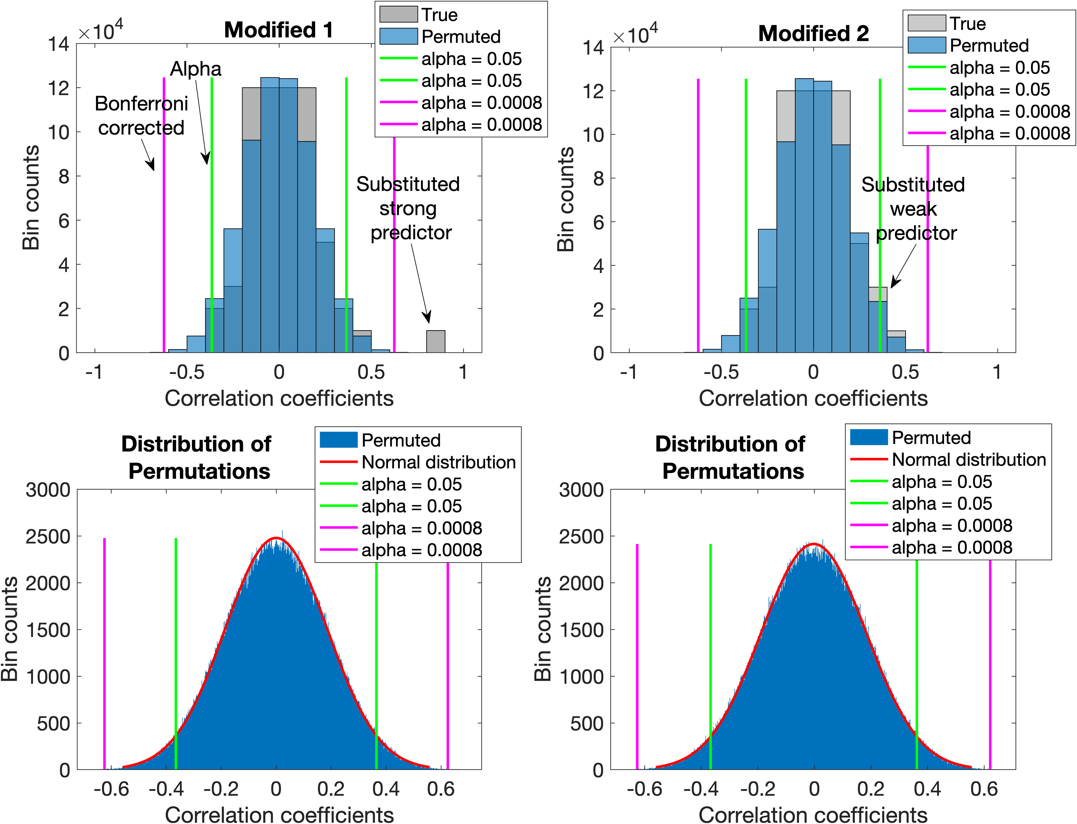
Histograms of correlation coefficients between predictor and true response data for the Modified 1 (dark grey to indicate modified void structure) and Modified 2 (light grey to indicate modified void structure) data sets and between predictor and permuted response data (blue) are shown in the top panels. Where distributions overlap, the color is darker. The distribution of the permutations’ correlation coefficients with normal probability distribution fits are in the respective bottom panels. The Void 2 set was modified by replacing a predictor with a very weak correlation coefficient with the response data with one that had a strong correlation coefficient to create the Modified 1 set. This was intended to mimic the presence of a happenstance correlation coefficient between predictor and response data. This correlation coefficient was high enough to exceed the Bonferroni corrected α level. The H_0B was rejected and the data considered suitable for PLS-DA (see further discussion in the text). For the Modified 2 data, the replacement had a weaker correlation coefficient (binned with others) and therefore no correlation coefficient exceeded the Bonferroni corrected significance level. For correlation coefficients exceeding the green lines, the median absolute correlation coefficient between predictor and true response data did not exceed that between predictor and permuted response data. Thus, neither the H_0B nor the H_0W was rejected and the Modified 2 data were considered inappropriate for PLS-DA.

The Modified 2 set was similar to the Modified 1 set but had a weaker correlation coefficient from the Weak set that replaced the original one present (cf. Table I). It had 2 correlation coefficients that exceeded the standard significance levels and none that exceeded the Bonferroni corrected levels as evident in Figure 5 (right panels). In this case, the H_0B could not be rejected and the secondary test was performed. In the secondary test, the median absolute true condition correlation coefficient was 0.3990, less than the 0.4122 of the median absolute permutation condition correlation coefficient. Thus, the H_0W (P = 0.7110) was also not rejected and the data considered inadequate for PLS-DA.

The results of the Modified 1 and Modified 2 sets deserve a number of comments. The Modified 1 set mimicked a data set that is in reality unsuitable for PLS-DA due to mimicking a happenstance correlation coefficient. However, the high correlation coefficient led to a rejection of H_0B. There are two implications of this situation. The first is that no α level can ever completely avoid the occurrence of a Type I error, the best that can be done is attempting to reduce the chances of such occurrences, for example, by applying the Bonferroni correction as we did here. The second is that it would be prudent to nevertheless examine situations where only one or at most a very few such outliers occur that might be due to happenstance. For the Modified 2 set, a comparison between the true and permuted conditions of all the absolute correlation coefficients that exceed the standard significance levels is needed. Useful data must have a true condition median significantly greater than that of the permutation condition median. One could think of this requirement as the true condition having a heavier or thicker tail than that of the permutation condition even though the correlation coefficients of the true condition might not be normally distributed.

Though the risk of a committing a Type I error with respect to the correlation coefficients can be reduced and it is advisable to examine situations where at most a very few significantly different correlation coefficients occur, the question arises as to what more can be said about such predictors. Given a binary response and using the binomial distribution, a test of the predictor with a significant correlation coefficient might further inform whether it is a chance effect. Examination of the substitution predictor in the Modified 1 set revealed a correct classification rate of 28/30. The concomitant probability of occurrence was 4.3400 × 10^–7, much less than the Bonferroni corrected significance level of 8.0645 × 10^–4 based on the cumulative binomial distribution. The same substitution predictor in the Modified 2 set had a correct classification rate of 21/30, not meeting the Bonferroni corrected significance level. No other predictor in that set did either. For the Void 1 and Void 2 sets, no predictor met these significance levels. Given limited data and the difficulties of obtaining additional samples, further support, where available, may derive from biological or biochemical information congruent with the presence of such apparently significant predictors.

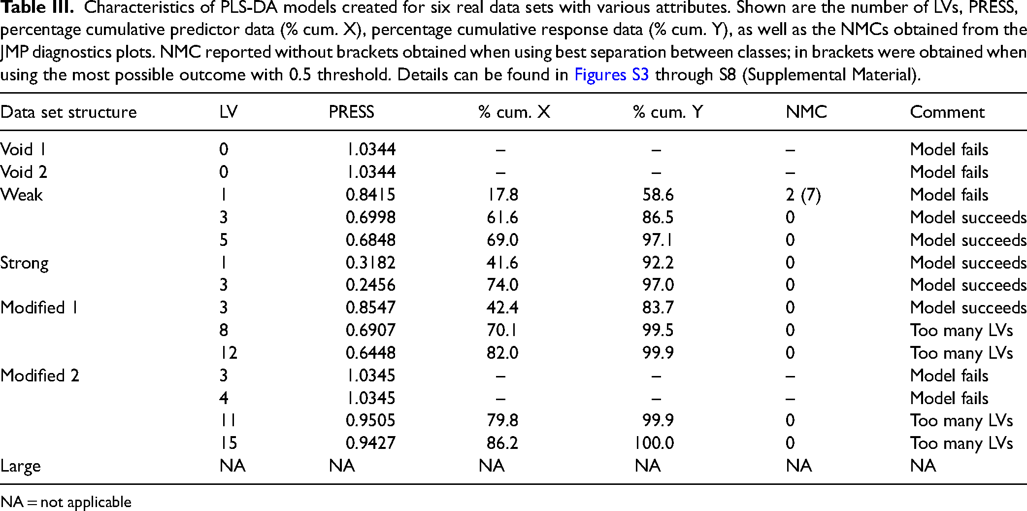
There is a rich literature base dealing with aspects of PLS-DA modeling, the choice of the optimal number of LVs, different PLS variants, various validation schemes and their effects on model quality.^{12,1430–32,38} It is not our objective to contribute to this literature, but rather to assess whether our estimates of data adequacy are borne out by the most widely used PLS-DA methods. The results, summarized in Table III, confirm the difficulty in creating models with the Void samples and the ease with which models can be created with the Strong samples. Complete details are shown in the Supplemental Material figures. These results are generally consistent with our expectations based on the preceding hypothesis tests.

Table III.

Characteristics of PLS-DA models created for six real data sets with various attributes. Shown are the number of LVs, PRESS, percentage cumulative predictor data (% cum. X), percentage cumulative response data (% cum. Y), as well as the NMCs obtained from the JMP diagnostics plots. NMC reported without brackets obtained when using best separation between classes; in brackets were obtained when using the most possible outcome with 0.5 threshold. Details can be found in Figures S3 through S8 (Supplemental Material).

Data set structure	LV	PRESS	% cum. X	% cum. Y	NMC	Comment
Void 1	0	1.0344	–	–	–	Model fails
Void 2	0	1.0344	–	–	–	Model fails
Weak	1	0.8415	17.8	58.6	2 (7)	Model fails
	3	0.6998	61.6	86.5	0	Model succeeds
	5	0.6848	69.0	97.1	0	Model succeeds
Strong	1	0.3182	41.6	92.2	0	Model succeeds
	3	0.2456	74.0	97.0	0	Model succeeds
Modified 1	3	0.8547	42.4	83.7	0	Model succeeds
	8	0.6907	70.1	99.5	0	Too many LVs
	12	0.6448	82.0	99.9	0	Too many LVs
Modified 2	3	1.0345	–	–	–	Model fails
	4	1.0345	–	–	–	Model fails
	11	0.9505	79.8	99.9	0	Too many LVs
	15	0.9427	86.2	100.0	0	Too many LVs
Large	NA	NA	NA	NA	NA	NA

NA = not applicable

Discussion

The approach that we present here consisted of permutations to completely destroy the correlation structure between predictor and response data and to compare those results with the intact correlation structure. Permutation generated correlation coefficient distributions that well approximated normal distributions were used to establish critical correlation coefficient values for the standard significance and Bonferroni corrected levels. Bonferroni corrected significance levels counter but cannot eliminate Type I or false positive errors. Correlation coefficients of the intact correlation structure that exceeded the Bonferroni corrected levels led to a rejection of the Bonferroni corrected null hypothesis H_0B. A rejection of the H_0B indicated that the given data set was adequate for PLS-DA. Failure to reject the H_0B did not alone imply inadequacy of the data for PLS-DA because it carried with it the risk of committing a Type II false negative error. Thus, failure to reject the H_0B made necessary a secondary test. This was based on a rank sum test of absolute correlation coefficients, which exceeded the standard significance level critical values, of the true condition compared to those of the permutation condition. If the median of the true condition absolute correlation coefficients was significantly greater than the median of the absolute correlation coefficients of the permutation condition, the H_0W was rejected and the data pronounced suitable. Otherwise, the data were deemed inadequate for PLS-DA. There is an inherent conflict present in trying to guard against both Type I and Type II errors. Considering both tests, one might question why the H_0W is not sufficient by itself. If the H_0W is rejected due to the presence of a single correlation coefficient, as opposed to the presence of several correlation coefficients, it might well be a correlation coefficient due to chance and the data should be considered inadequate unless the H_0B is also rejected due to a strong correlation coefficient that merits further investigation. Thus, a Type I error is unlikely, but possible. Performing the H_0B first might preclude the necessity for also performing the H_0W. However, we concede that the reverse sequence could also be implemented. Though the chances of committing a Type II error can be reduced, they also cannot be eliminated.

Increasing the sample size will cause all correlation coefficients to approximate their true values. There are two effects that come into play here. The first occurs when correlation coefficients are initially spuriously strong or weak. The most troubling cases are chance correlation coefficients that are initially spuriously strong and true correlation coefficients that are initially spuriously weak because both would give rise to erroneous models when, respectively, a chance correlation coefficient is used or when a true correlation coefficient is missed. As the sample size increases, the probability of a spuriously strong chance correlation coefficient being present will be reduced as will the probability of a spuriously weak true correlation coefficient.

The second occurs because increasing the sample size reduces the absolute values of all chance correlation coefficients (i.e., true zero or near-zero ones). Thus, when true, but weak, correlation coefficients are present amongst other weak correlation coefficients within the normal confidence intervals of the destroyed structure, these can be found if the sample size is increased. These effects are shown in Figure 6 for a small sample (n = 20) and a large one (n = 54) with a substitution to create a “true” predictor (the large data set). The Large set is similar to that of the Void 1 and Void 2 sets (i.e., without set structure), but with a substituted predictor (cf. Table I). The Small set is a subset of the Large set consisting of the first 10 observations in each group. It can be seen from Figure 6 that the correlation coefficient of the “true” predictor increased (in absolute terms) from –0.4000 to –0.5508 and that the distribution of a destroyed correlation structure’s correlation coefficients narrowed with concomitant reduction of the interval between the standard significance level critical values (green lines) with increasing sample size. Both effects would eventually cause the true correlation coefficient(s) to separate from others sufficiently to result in H_0W and eventually H_0B rejection. Figure S2 shows more detail where the gradual emergence of a true predictor is evident from the distribution of chance correlations when the sample size increases. Hence, given a specific data set, we can avoid Type I and Type II errors only to a certain extent.

Figure 6.

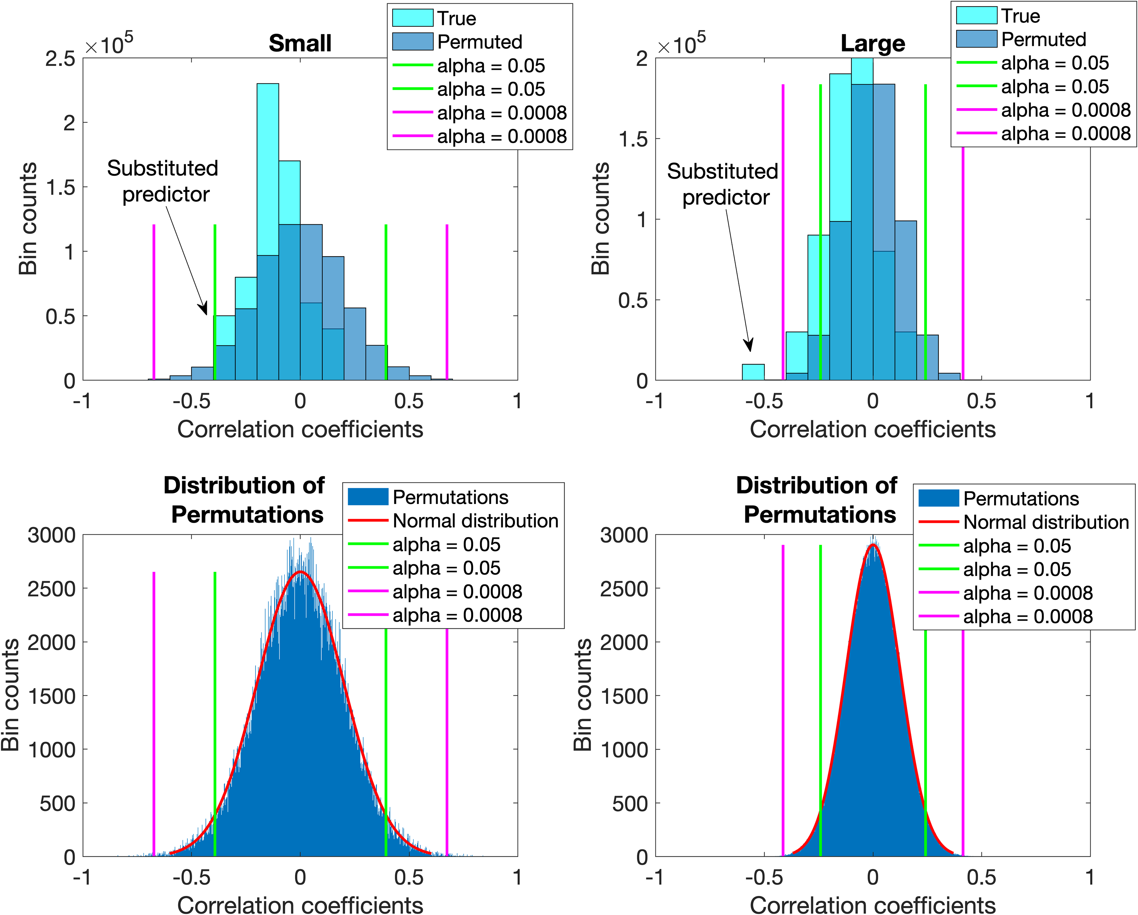
Change in the distribution of correlation coefficients between predictor and true response data (cyan) and between predictor and permuted response data (blue) as the sample size increases from 20 to 54. Correlation coefficients due to chance decrease in absolute value causing their distribution to narrow while true correlation coefficients increase if initially spuriously low resulting in an apparent emergence of the true correlation coefficients from the distribution of chance coefficients. This is shown here where a “true” predictor was substituted for a chance predictor in a collection of other chance predictors.

From both the Modified 1 and Modified 2 cases we infer that suitably strong correlation coefficients must be present in the data to reject the null hypotheses (Figure 5). This was consistent with the observations of others.^26,27 If true but weaker effects are present, more samples are needed (Figure S2) and this might need to be even further increased where subpopulations are involved. Marek et al.,²⁰ concluded that brain region association studies required thousands of observations. In response, others pointed out that the sample sizes needed depended on the effect sizes present.^26,27 Figure 7 (left panel) plots the change in the critical values (here we used only the positive ones) for the correlation coefficients of the Large data set to reach the standard and Bonferroni corrected alphas using increasing sample sizes. The standard alpha critical values intersected with a correlation coefficient of 0.3 at a sample size of 38. A single exponential fit was then applied to the successive Bonferroni alpha levels to see where it would intersect with a correlation coefficient of 0.3. We found that this intersection occurred for a sample size of around 68. Thus, we concluded that approximately 68 samples were necessary in the presence of 64 predictors to reject the H_0B. This gave a ratio of samples to predictors of 1.1. However, a biexponential fit was better and suggested a sample size of 83 would be needed and gave a ratio of 1.3. Though this value for Raman spectra and a single response variable appeared substantially different from that estimated to be needed in brain association studies,^12,20 these inferences were based on a Raman spectroscopy data set with 64 predictors and a single response. Biexponentials also produced very good fits for synthetic data with a slightly extended range (Figure 7, right panel). From these simulations, we found that to reject the H_0B at a correlation coefficient of 0.3 and using an observational set of 50 predictors, 107 samples would be needed. However, it is important to understand that augmenting an inadequate data set with more samples that come from the same population when it is essentially void of information about the response would be futile. Nevertheless, having augmented the data set and finding that it is still inadequate ought to be a definitive conclusion of inadequacy.

Figure 7.

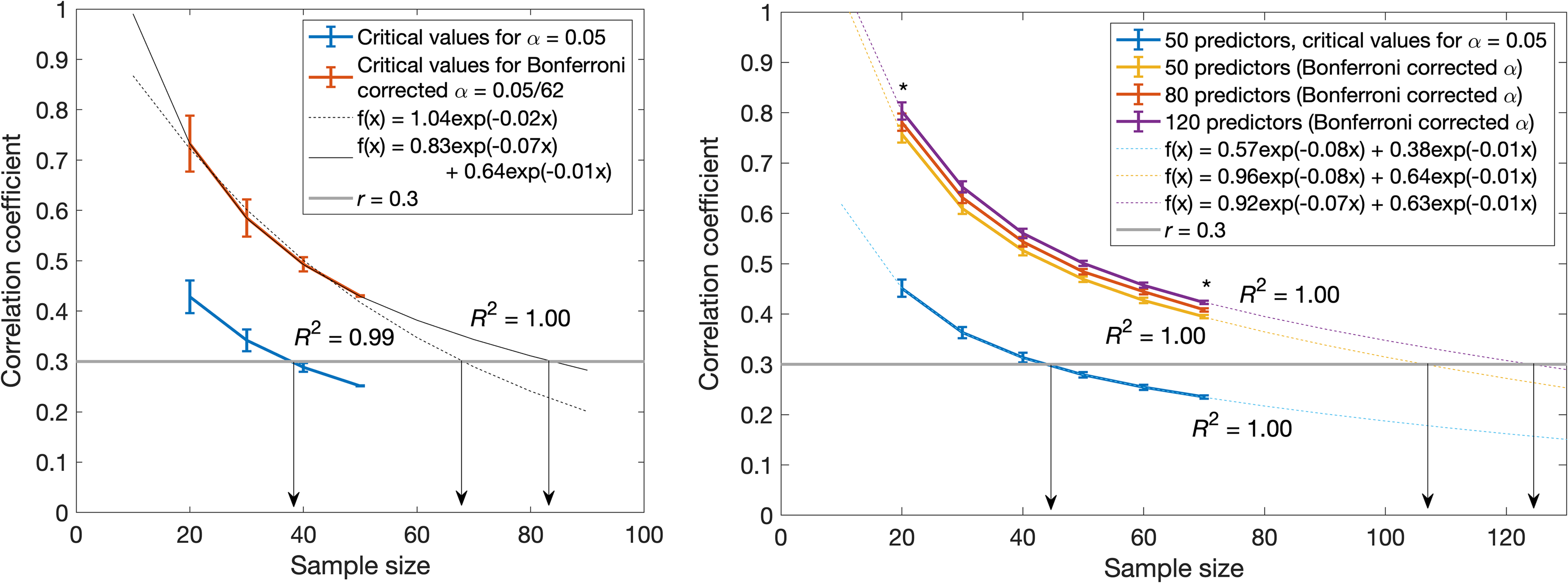
Change in the critical values of correlation coefficients to reach the standard and Bonferroni corrected significance levels for different sample sizes obtained from the Large data set (left panel) and to reach the standard and Bonferroni corrected significance levels for different sample sizes obtained from simulations with a varying number of predictors (right panel). Shown is an example critical correlation coefficient of 0.3 (gray line). With an increasing number of predictors, the simulated curves shifted significantly (asterisks, P < 0.0001) upward implying that more samples would be needed to obtain significance at the level of a 0.3 correlation coefficient. The experimental and simulated data were fitted with exponentials.

We expected that for data sets with an equal number of observations, the set with the larger number of predictors would have a greater range of chance correlation coefficients. Thus, it will have a normal distribution that is flatter and wider than the normal distribution of the set with fewer predictors. When taking a small subset of observations from one of these data sets, the normal distribution so obtained will be flatter and wider than that of the parent distribution as seen in Figure 5 and Figure S2 (Supplemental Material). Consequently, we expected the curves in Figure 7 to shift upward with a concomitant extension of their intersections with the 0.3 correlation coefficient toward larger sample sizes. This was borne out by the simulations shown in the Figure 7, right panel. Significant increases (one-tailed, two-sample t-tests) were observed for sample sizes of 20 (P < 0.0001) and 70 (P < 0.0001) when the number of predictors in the data set increased from 50 to 120 (left and right asterisks, respectively). Details about the simulations and the statistics can be found in the Supplemental Material.

Our objective with this work was to assess the adequacy of a given set of observational data for use in PLS-DA model building. To this end, we used nine data sets, three synthetic sets, and six each consisting of fitted peaks of 30 Raman spectra from mammalian cells. The sets were assembled in various ways to have specific relationships with a categorical response. We then performed hypothesis tests to determine the adequacy of any given data set for PLS-DA modeling. The basic PLS-DA models constructed from these data sets were then used to determine whether the outcomes of our hypothesis tests could serve as data prescreening tests to justify PLS-DA modeling. Our objective was to evaluate the data, not the models.

Thus, our approach differs fundamentally from others where synthetically generated and real data were used to examine the strengths and weaknesses of PLS-DA, assess model quality, or report model performance given certain data characteristics.^12,14,17,18 To assess the adequacy of observational data sets for use in PLS-DA, we exploited the availability of both predictor and response data, as well as the PLS-DA dependence on the underlying association between them.

Our approach specifically differs conceptually and practically from other methods based on data permutations. For example, Westerhuis et al.³⁰ and Szymanska et al.³² used permutations of class labels. In both these cases, the permutations allowed a reference null distribution of PLS-DA model performance to be established based on “faulty” data that should impair its prediction of classes. Against this null distribution, the outcome of the PLS-DA model using the original data is evaluated to determine if it is significantly better than when based on permuted data. However, these permutation strategies were primarily designed to evaluate cross-validation schemes and diagnostic statistics for PLS-DA, rather than to assess the adequacy of the data itself. Moreover, these approaches use PLS-DA models based on data that might already incorporate chance effects and so might not effectively control for them. Cross-validation strategies, diagnostic statistics and pruning also implicitly address data that produce strong models (i.e., can a good model be built?), not potentially erroneous data. For example, with PLS-DA model pruning, variables important in projection with small values and small regression coefficients are considered candidates for deletion.⁵ Thus, if a good model can be built with the data at hand and if data not meeting the pruning criteria are retained, chance effects might nevertheless persist in models. In sharp contrast, our novel approach explicitly evaluates the adequacy of data for PLS-DA modeling prior to model construction, providing a fundamentally different safeguard against spurious or misleading results. Additionally, our method uniquely aims to control both Type I and Type II errors, a feature generally absent from internal cross-validation schemes. While external cross-validation attempts to mitigate false positives using an independent dataset, that dataset itself may still carry random effects that compromise the reliability of the outcome.

Data permutations are also used in the context of gene enrichment analysis, for example, by Subramanian et al.³⁹ These authors used correlations between predictor gene expression levels and response class labels followed by determining an enrichment score as the maximum deviation from zero in a Kolmogorov–Smirnov manner. Permutations of the response were used to determine a null distribution of correlations that permitted significance tests of the enrichment score. The Westfall–Young method addresses the problem of dependent p-values in multiple hypothesis testing by permuting the response, performing individual hypothesis tests on all the predictors, and finding the individual p-values of these tests. Using numerous permutations of the response, the minimum p-value over all predictors is recorded for every permutation to create a distribution of p-values from which a critical value for the desired α is found. The p-value corresponding to this critical value then serves as cutoff and the null hypotheses of predictors in the non-permuted data with p-values smaller than the cutoff are rejected.^40,41 In contrast to the Westfall–Young method, we do not perform multiple hypothesis tests and do not directly address the problem of dependent p-values with permutations because the peak fitting results in both dimensionality and collinearity reduction. We also explicitly use associations between predictors and response.

Our study has several limitations, including some that may not be immediately evident. Among the identifiable ones, we recognize concerns regarding the method’s generalizability and the current limitations of the hypothesis tests. Though the simulations and real data produced qualitatively similar results suggesting that this approach has general validity, it is not currently understood under which conditions this might be true. Relatedly, the Bonferroni adjustment is conservative and division by the number of predictors makes it more so when some of the predictors are collinear. With peak fitting of Raman spectra, we have reduced the dimensions of our data by ∼15× and the collinearity of peaks from ∼7× to ∼21× (depending on the width of a given peak). However, some peaks belonging to the same component will still have collinearity and this we have not taken into consideration. The use of other methods to control for Type I errors, such as the Holm–Bonferroni method, which is more powerful than the Bonferroni method and has less risk of committing Type II errors should be investigated. Concern about too stringent controls of false positives indeed prompted us to also control for false negatives. This test too needs further development and full characterization. Thus, we expect that improving both the hypothesis tests might reduce the current Type II error rate without affecting the Type I error rate.

Associated with both tests is the use of normal distributions as approximations for the permuted distributions. This might not hold under all conditions, for example with a small number of observations. Furthermore, a sample size of ∼650 000, as here, might render significant differences between the permuted nearly normal distribution and a true normal distribution practically pointless. Thus, practical limits need to be established or nonparametric tests might be more appropriate and their use should be investigated instead. A complete analysis of these and other relationships will have to await future efforts.

Conclusion

The correlation structure between predictor and response data can be destroyed with permutations. It produces a normal distribution of chance correlation coefficients that can be used to find correlation coefficients in the intact data that differ significantly from others. To counter Type I errors, the standard significance level can be adjusted using the Bonferroni correction. To counter the probability of a Type II error, we can compare the tails of true to permuted standard significant correlation coefficients. We devised two hypothesis tests to implement this two-stage error control approach. If data sets pass one or both of these hypothesis tests, the entire data set is considered adequate for use.

For simulated data sets, we found that our approach reduced false positives compared to PLS-DA models by about 12-fold, a significant difference. False negatives exceeded by about 4.5 fold that of PLS-DA, also significant. For our simulated and real data sets, we found that (i) where no relationship existed between predictor and response data, no Bonferroni-significant correlation coefficients were observed and modeling was unsuccessful; (ii) where a strong relationship existed between predictor and response data, numerous correlation coefficients significant at the standard and Bonferroni levels were observed and modeling was easy; (iii) where a weak relationship existed between predictor and response data, a few significant correlation coefficients occurred even at the Bonferroni level and modeling tended to be successful; and (iv) we found how to estimate the sample size needed to detect a given true correlation coefficient. (v) In addition, for the real data we also found that where, due to chance, one or a very few Bonferroni-significant correlations were observed in a set, the probability of a chance occurrence of those predictor(s) could be further evaluated using the binomial distribution.

The results from simulated and real data suggest that our method can be generalized. We therefore conclude that, by pre-screening the data at hand as described herein, one can assess whether it would be appropriate to proceed with PLS-DA model building. We deem it to be unwise to proceed with PLS-DA when there are no predictors with correlation coefficients that can be differentiated from chance occurrences in a given data set. In such cases it would be better to increase the sample size and we provide a way of estimating by how many. Our approach provides a safeguard against the waste of resources and against adverse outcomes from building and using apparently excellent models that are unable to generalize to new data.

Supplemental Material

sj-docx-1-asp-10.1177_00037028261439686 - Supplemental material for Data Adequacy Testing for Partial Least Squares Discriminant Analysis Using Raman Spectra

Supplemental material, sj-docx-1-asp-10.1177_00037028261439686 for Data Adequacy Testing for Partial Least Squares Discriminant Analysis Using Raman Spectra by H. Georg Schulze, Rupa Haldavekar, Shreyas Rangan, Smilla Colombini, Michael W. Blades, Robin F. B. Turner and James M. Piret in Applied Spectroscopy

Footnotes

Acknowledgments

We acknowledge the Canadian Foundation for Innovation and the British Columbia Knowledge Development Fund for funding the purchase of instrumentation made available for this work through the UBC Laboratory for Molecular Biophysics. The authors acknowledge that some material was based on information from an artificial intelligence agent that they subsequently evaluated and verified. We wish to express our gratitude to anonymous reviewers for their valuable comments. We are obliged to Pany Allen and Chuck London at JMP Statistical Discovery Software for making the JMP Student Edition software available.

Declaration of Conflicting Interests

The authors declare no potential conflicts of interest with respect to the research, authorship, and/or publication of this article.

Funding

The authors thank the National Research Council of Canada and the Natural Sciences and Engineering Research Council of Canada for financial support.

ORCID iDs

Rupa Haldavekar

Shreyas Rangan

Michael W. Blades

Robin F. B. Turner

Supplemental Material

All supplemental material mentioned in the text is available in the online version of the journal.

References

1.
Mendez K.M. Broadhurst D.I. Reinke S.N. . “Migrating from Partial Least Squares Discriminant Analysis to Artificial Neural Networks: A Comparison of functionally Equivalent Visualisation and Feature Contribution Tools Using Jupyter Notebooks”. Metabolomics. 2020. 16(2): 17. 10.1007/s11306-020-1640-0

2.
Hanrahan G. Udeh F. Patil D.G. . “Chemometrics and Statistics: Multivariate Calibration Techniques”. Encyclopedia of Analytical Science. Amsterdam: Elsevier, 2005. Pp. 27–32. 10.1016/B0-12-369397-7/00077-7

3.
Wold. H. "Model Construction and Evaluation When Theoretical Knowledge is Scarce: Theory and Application of Partial Least Squares". In: J. Kmenta, J.B. Ramsay, editors. Evaluation of Econometric Models. New York; Academic Press, 1980. Pp. 47-74. https://doi.org/10.1016/B978-0-12-416550-2.50007-8

4.
De Jong S. . “SIMPLS: An Alternative Approach to Partial Least Squares Regression”. Chemom. Intell. Lab. Syst. 1993. 18(3): 251–263. 10.1016/0169-7439(93)85002-X

5.
Wold S. Sjöström M. Eriksson L. . “PLS-Regression: A Basic Tool of Chemometrics”. Chemom. Intell. Lab. Syst. 2001. 58(2): 109–130. 10.1016/S0169-7439(01)00155-1

6.
Martin M. Wongwattanakul M. Khemtonglang N. Kiatchoosakun P. , et al. “Identification of Glucose-6 Phosphate Dehydrogenase Deficient Patients Using Attenuated Total Reflection Fourier Transform Infrared Spectroscopy Using Partial Least Squares Discriminant Analysis in Aqueous Blood Samples”. Appl Spectrosc. 2023. 77(5): 513–520. 10.1177/00037028231170851

7.
Yu K. Wu H. Xiong H. Wang G. , et al. “Ante- and Post-Mortem Fracture Identification Protocol Based on Low- and High-Level Fusion Using Fourier Transform Infrared Spectroscopy and Raman Spectroscopy Association”. Appl Spectrosc. 2024. 78(6): 605–615. 10.1177/00037028241231994

8.
Park J. Kumar S. Han S.-H. Singh V.K. , et al. “Two-Step Partial Least Squares-Discriminant Analysis Modeling for Accurate Classification of Edible Sea Salt Products Using Laser-Induced Breakdown Spectroscopy”. Appl Spectrosc. 2022. 76(9): 1042–1050. 10.1177/00037028221091581

9.
Lloyd G.R. Stone N. . “Method for Identification of Spectral Targets in Discrete Frequency Infrared Spectroscopy for Clinical Diagnostics”. Appl Spectrosc. 2015. 69(9): 1066–1073. 10.1366/14-07677

10.
Kleimeyer J.A. Rose P.E. Harris J.M. . “Determination of Ultratrace-Level Fluorescent Tracer Concentrations in Environmental Samples Using a Combination of HPLC Separation and Laser-Excited Fluorescence Multiwavelength Emission Detection: Application to Testing of Geothermal Well Brines”. Appl Spectrosc. 2001. 55(6): 690–700. 10.1366/0003702011952613

11.
Abdi H. . “Partial Least Squares Regression and Projection on Latent Structure Regression (PLS Regression)”. WIREs Comput Stat. 2010. 2(1): 97–106. 10.1002/wics.51

12.
Helmer M. Warrington S. Mohammadi-Nejad A.-R. Ji J.L. , et al. “On the Stability of Canonical Correlation Analysis and Partial Least Squares with Application to Brain-Behavior Associations”. Commun Biol. 2024. 7(1): 217. 10.1038/s42003-024-05869-4

13.
Worley B. Powers R. . “Multivariate Analysis in Metabolomics”. CMB. 2012. 1(1): 92–107. 10.2174/2213235X11301010092

14.
Rodríguez-Pérez R. Fernández L. Marco S. . “Overoptimism in Cross-Validation When Using Partial Least Squares-Discriminant Analysis for Omics Data: A Systematic Study”. Anal. Bioanal. Chem. 2018. 410(23): 5981–5992. 10.1007/s00216-018-1217-1

15.
Yang Q. Gong Y. Zhu F. . “Critical Assessment of the Biomarker Discovery and Classification Methods for Multiclass Metabolomics”. Anal. Chem. 2023. 95(13): 5542–5552. 10.1021/acs.analchem.2c04402

16.
Ouertani S.S. Mazerolles G. Boccard J. Rudaz S. Hanafi M. . “Multi-Way PLS for Discrimination: Compact Form Equivalent to the Tri-Linear PLS2 Procedure and its Monotony Convergence”. Chemom. Intell. Lab. Syst. 2014. 133: 25–32. 10.1016/j.chemolab.2014.01.015

17.
Brereton R.G. Lloyd G.R. . “Partial Least Squares Discriminant Analysis: Taking the Magic Away”. J. Chemom. 2014. 28(4): 213–225. 10.1002/cem.2609

18.
Ruiz-Perez D. Guan H. Madhivanan P. Mathee K. Narasimhan G. . “So You Think You Can PLS-DA?”. BMC Bioinf. 2020. 21(S1): 2. 10.1186/s12859-019-3310-7

19.
Gaida M. Stefanuto P.-H. Focant J.-F. . “Theoretical Modeling and Machine Learning-Based Data Processing Workflows in Comprehensive Two-Dimensional Gas Chromatography: A Review”. J. Chromatogr. A. 2023. 1711: 464467. 10.1016/j.chroma.2023.464467

20.
Marek S. Tervo-Clemmens B. Calabro F.J. Montez D.F. , et al. “Reproducible Brain-Wide Association Studies Require Thousands of Individuals”. Nature. 2022. 603(7902): 654–660. 10.1038/s41586-022-04492-9

21.
Mihalik A. Ferreira F.S. Moutoussis M. Ziegler G. Adams R.A. Rosa M.J. , et al. “Multiple Holdouts with Stability: Improving the Generalizability of Machine Learning Analyses of Brain–Behavior Relationships”. Biol. Psych. 2020. 87(4): 368–376. 10.1016/j.biopsych.2019.12.001

22.
Lasalvia M. Capozzi V. Perna G. . “A Comparison of PCA-LDA and PLS-DA Techniques for Classification of Vibrational Spectra”. Appl. Sci. 2022. 12(11): 5345. 10.3390/app12115345

23.
Liu C. Zhang X. Nguyen T.T. Liu J. , et al. “Partial Least Squares Regression and Principal Component Analysis: Similarity and Differences Between Two Popular Variable Reduction Approaches”. Gen Psych. 2022. 35(1): e100662. 10.1136/gpsych-2021-100662

24.
Mevik B.-H. Wehrens R. . “Introduction to the PLS Package”. https://khliland.github.io/pls/articles/pls-manual.html [accessed 20 March 2026].

25.
Beleites C. Neugebauer U. Bocklitz T. Krafft C. Popp J. . “Sample Size Planning for Classification Models”. Anal. Chim. Acta. 2013. 760: 25–33. 10.1016/j.aca.2012.11.007

26.
DeYoung C.G. Sassenberg T. Abend R. Allen T. , et al. “Reproducible Between-Person Brain-Behavior Associations Do Not Always Require Thousands of Individuals”. PsyArXiv. 2022. 10.31234/osf.io/sfnmk

27.
Gratton C. Nelson S.M. Gordon E.M. . “Brain-Behavior Correlations: Two Paths Toward Reliability”. Neuron. 2022. 110(9): 1446–1449. 10.1016/j.neuron.2022.04.018

28.
Rosenberg M.D. Finn E.S. . “How to Establish Robust Brain–Behavior Relationships Without Thousands of Individuals”. Nat Neurosci. 2022. 25(7): 835–837. 10.1038/s41593-022-01110-9

29.
Spisak T. Bingel U. Wager T. . “Replicable Multivariate BWAS with Moderate Sample Sizes”. BioRxiv. 2022. 10.1101/2022.06.22.497072

30.
Westerhuis J.A. Hoefsloot H.C.J. Smit S. Vis D.J. , et al. “Assessment of PLSDA Cross Validation”. Metabolomics. 2008. 4(1): 81–89. 10.1007/s11306-007-0099-6

31.
Westad F. Marini F. . “Validation of Chemometric Models: A Tutorial”. Anal. Chim. Acta. 2015. 893: 14–24. 10.1016/j.aca.2015.06.056

32.
Szymańska E. Saccenti E. Smilde A.K. Westerhuis J.A. . “Double-Check: Validation of Diagnostic Statistics for PLS-DA Models in Metabolomics Studies”. Metabolomics. 2012. 8(S1): 3–16. 10.1007/s11306-011-0330-3

33.
Westerhuis J.A. Van Velzen E.J.J. Hoefsloot H.C.J. Smilde A.K. . “Discriminant Q²(DQ²) for Improved Discrimination in PLSDA Models”. Metabolomics. 2008. 4(4): 293–296. 10.1007/s11306-008-0126-2

34.
Glass G.V. Hopkins K.D. . Statistical Methods in Education and Psychology. New Jersey: Prentice-Hall, 1984.

35.
Rangan S. Wong R. Schulze H.G. Vardaki M.Z. , et al. “Saline Dry Fixation for Improved Cell Composition Analysis Using Raman Spectroscopy”. Analyst. 2023. 148(12): 2745–2757. 10.1039/D2AN01916G

36.
Schulze H.G. Rangan S. Piret J.M. Blades M.W. Turner R.F.B. . “Developing Fully Automated Quality Control Methods for Preprocessing Raman Spectra of Biomedical and Biological Samples”. Appl. Spectrosc. 2018. 72(9): 1322–1340. 10.1177/0003702818778031

37.
Schulze H.G. Rangan S. Vardaki M.Z. Blades M.W. , et al. “Critical Evaluation of Spectral Resolution Enhancement Methods for Raman Hyperspectra”. Appl. Spectrosc. 2022. 76(1): 61–80. 10.1177/00037028211061174

38.
Denham M.C. . “Choosing the Number of Factors in Partial Least Squares Regression: Estimating and Minimizing the Mean Squared Error of Prediction”. J. Chemom. 2000. 14(4): 351–361. 10.1002/1099-128X(200007/08)14:4%3C351::AID-CEM598%3E3.0.CO;2-Q

39.
Subramanian A. Tamayo P. Mootha V.K. Mukherjee S. , et al. “Gene Set Enrichment Analysis: A Knowledge-Based Approach for Interpreting Genome-Wide Expression Profiles”. Proc. Natl. Acad. Sci. U.S.A. 2005. 102(43): 15545–15550. 10.1073/pnas.0506580102

40.
Goeman J.J. Solari A. . “Multiple Hypothesis Testing in Genomics”. Statist. Med. 2014. 33(11): 1946–1978. 10.1002/sim.6082

41.
Westfall P.H. Young S.S. . Resampling-Based Multiple Testing: Examples and Methods for P-Value Adjustment. New York: John Wiley and Sons, 1993.

Supplementary Material

Please find the following supplemental material available below.

For Open Access articles published under a Creative Commons License, all supplemental material carries the same license as the article it is associated with.

For non-Open Access articles published, all supplemental material carries a non-exclusive license, and permission requests for re-use of supplemental material or any part of supplemental material shall be sent directly to the copyright owner as specified in the copyright notice associated with the article.

0.00 MB

1.22 MB