
Abstract
Abstract
Spatially explicit capture–recapture (SECR) models have gained enormous popularity to solve abundance estimation problems in ecology. In this study, we develop a novel Bayesian SECR model that disentangles two processes: one is the process of animal arrival within a detection region, and the other is the process of recording this arrival by a given set of detectors. We integrate this complexity into an advanced version of a recent SECR model involving partially identified individuals (Royle JA. Spatial capture-recapture with partial identity. arXiv preprint arXiv:1503.06873, 2015). We assess the performance of our model over a range of realistic simulation scenarios and demonstrate that estimates of population size N improve when we utilize the proposed model relative to the model that does not explicitly estimate trap detection probability (Royle JA. Spatial capture-recapture with partial identity. arXiv preprint arXiv:1503.06873, 2015). We confront and investigate the proposed model with a spatial capture–recapture dataset from a camera trapping survey of tigers (Panthera tigris) in Nagarahole study area of southern India. Detection probability is estimated at 0.489 (with 95% credible interval (CI) [0.430, 0.543]) which implies that the camera traps are performing imperfectly and thus justifying the use of our model in real world applications. We discuss possible extensions, future work and relevance of our model to other statistical applications beyond ecology.
AMS classification codes: 62F15, 92D40
Introduction
Understanding the dynamics of wildlife populations is central to answering ecological questions and forms the basis for conservation. However, owing to sampling problems (primarily imperfect detection and spatial sampling)1, 2 it is a major challenge to accurately characterize wildlife populations from field data. The challenge is greater when the species is cryptic, occurs at low density and often elusive, as with large carnivores3, 4 and rare ungulates. 5 This problem has motivated the development of several tailor-made statistical estimators over the years.1, 6, 7, 8
More recently, such classes of ecological problems have been addressed elegantly using hierarchical models, where a distinction between the “state process” (the true state of the ecological system that is of main interest) and the “observation process” (the way in which observations occur during sampling) is explicitly defined in the modelling.9, 10 Based on this philosophy, the development of spatially explicit capture–recapture models (hereafter SECR models)11–13 for estimating animal abundance has witnessed explosive growth 8 . Under this approach, observation data about individuals are recorded by spatial array of detectors (such as camera traps, hair snares and fixed traps) within an area of interest over a fixed time period. SECR models utilize the spatial locations of animal detections to explicitly enable inference about the spatial distribution of animals in addition to estimating animal abundance and has seen wide application for globally threatened species.8, 14
However, all these inferences are drawn from data emanating when animals pass through a spatial array of detectors. Currently, SECR models do not disentangle the process of animal arrival within a detection region from the process of recording this arrival by a given set of detectors. Furthermore, local detector-level effects may explain whether an animal will pass through the detection region or not. For example, workers often use baits to attract animals to trap stations when animals are in the vicinity and investigators are often interested to understand animal response to such detectors. However, an animal passing through a detection region will not necessarily mean that the detectors will record this event perfectly. The variables affecting detection and animal arrival are generally quite different. Different types of detectors (e.g., hair snare versus camera) perform differently under similar conditions. Further, temperature levels at the detection region can also have substantial effect on detector performance (e.g., on passive infrared cameras). When detection rates in recorded samples are low due to failure or malfunction of the detectors, these can result in data with uncertain identities or “partially identified individuals”. 15 Recently, Augustine et al., 16 more specifically describing paired camera trap surveys, utilizes separate parameters to model the relative encounter frequencies when both cameras function versus when only one of the two cameras functions. As an improvement, in this article, we provide a probabilistic approach that describes the exact mechanism by which we obtain these different events. If we assume that over a fixed number of detection attempts at a location we will detect an animal with certainty, then a newer development 17 can be used to address such problem. However, this is a restrictive assumption to meet in the real world.
Such surveys also result in partially identified individuals that require reconciliation in the modelling process. This area has received attention in the recent past, for example, McClintock et al. 18 has developed a model for photographic and genetic capture–recapture survey, Wimmer et al. 19 has developed a model that deals with partially identified individuals in the context of live captures. More recently, Royle JA 15 and Augustine et al. 16 have developed a model for partially identified sample where they demonstrate that spatial locations of captures assist in improved reconciliation of partially identified individuals.
Methods
In typical photographic capture–recapture surveys13, 22 an array consisting of camera trap stations is placed to sample a species of interest. Each station comprises of two cameras (detectors) facing each other and they are meant to independently capture both flank images of animals. If the species is naturally marked, individuals can be identified by their unique markings. While this example motivated our specific model development, we can also envision many scenarios where more than one detector and different detection types may be used to extract features of individual identity of animals. 14
Modelling Approach
We utilize the hierarchical modelling philosophy 9 to formulate a model to address the problem of imperfect detection of detectors in spatial capture–recapture models. A list of notations used in this article is provided in Table 1 (and another table of notations is given in Appendix Table 11).
State Process
Consider a population of individuals of certain species that reside within a bounded geographic region
Observation Process
We suppose that a spatial array of J trap stations are placed in the state space
Let
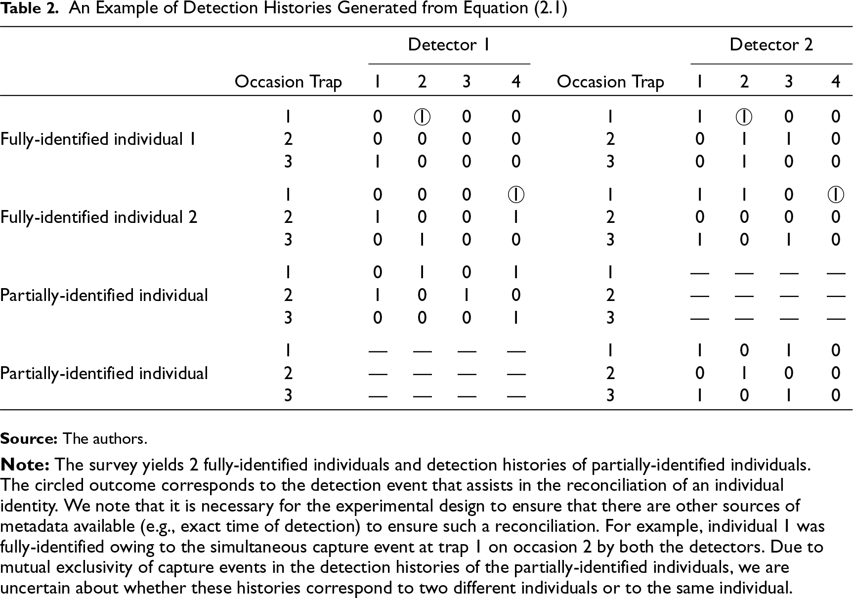
Example 2.1. In a survey, consider paired detectors (1 and 2), deployed at each of 3 (= J) trap stations and active for 4 (= K) sampling occasions. From this survey, we suppose that 2 (= n) distinct individuals were fully identified since we obtained at least one simultaneous capture (caught at the same time in both detectors) during the survey. Detection histories are thus presented in Table 2. For each of the fully identified individuals, the dimension of the detection history data set is 2 × 3 × 4.
The observation process described above with the example entails two problems that need to be addressed simultaneously: (a) determining whether an animal passes through the detection region (in trap station) in the face of imperfect detection of detectors and (b) reconciling partially-identified individuals. While the second problem has been recently addressed by Royle JA 15 and Augustine et al. 16 , our emphasis in this article is to address the first and integrate it into the solution of the second.
Notations of data which are used in this article
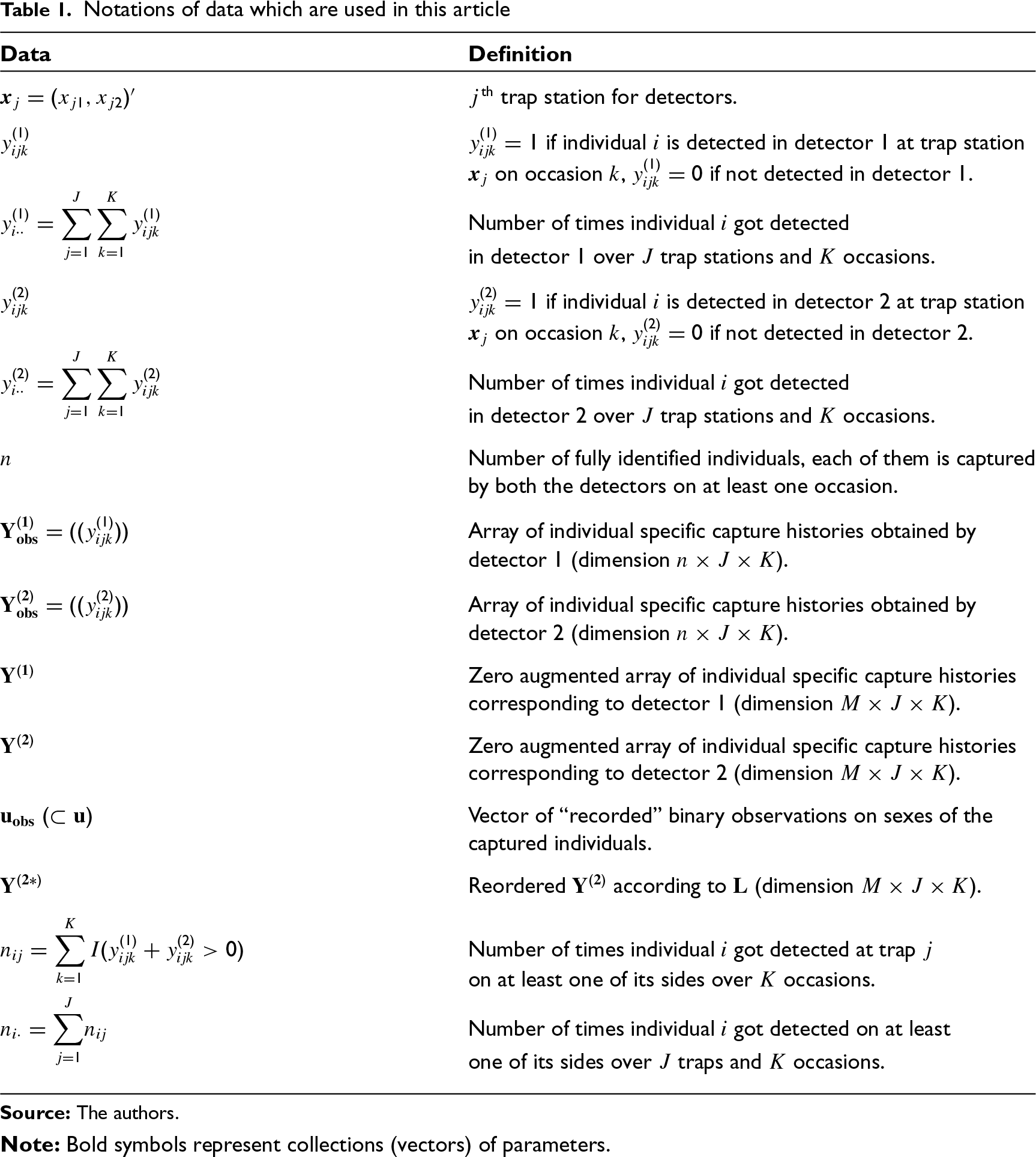
Notations of data which are used in this article
An Example of Detection Histories Generated from Equation (2.1)
Disentangling Animal Entry to Trap Station and Detection in Spatially Explicit Capture–Recapture Models
We note that for an animal to be observed by a detector at a given location and occasion, the animal (a) has to pass through the detection region and (b) has to be captured by the detector(s). We aim to disentangle these two processes by utilizing a hierarchical model. From Example 2.1, there are four types of detection histories observable at a given trap station on a given sampling occasion: “11” (observed by both detectors), “10” (observed by detector 1 but not by detector 2), “01” (not observed by detector 1 but observed by detector 2) and “00” (not observed by either detector). The first three histories (“11”, “10” and “01”) conclusively state that the animal passed through detection region in the trap station since we have one observation. But in the fourth case (“00”), we are presented with two possibilities: (a) the animal passed through the detection region and both detectors failed to record this event or (b) the animal did not pass through the detection region.
We proceed with the Gaussian form in our development, while recognizing that there can be many other options to define the rate of decline in animal trap entry probability to represent other realities. Further, it is often the case that sex acts as an important covariate to define the extent of animal movement.14, 23, 24 For example, often males and females have different extents of spatial movement, defined by the parameter σ in our development. We then define σ as the following:
Development of the Joint Posterior Density of All Parameters
Note that,
For each observed individual i, the detection history 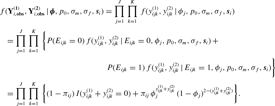
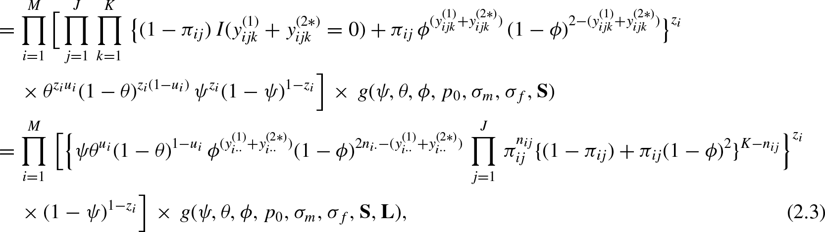
Note that the population size N, which is a parameter of major interest, is an unknown quantity. Due to this, the number of some other variables including some latent variables is unknown and therefore the dimension of the parameter space is also unknown. This is one of the main difficulties in analysing the proposed SECR model. We consider the method of data augmentation
13
for analysing the proposed SECR model to handle this difficulty. This is implemented by choosing a large integer M to bound N and augmenting the two observed data sets with a large number of “all-zero” encounter histories. We denote the zero-augmented data sets by 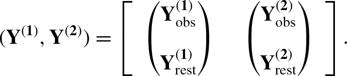
Here 
It is straightforward to handle the latent missing observations in 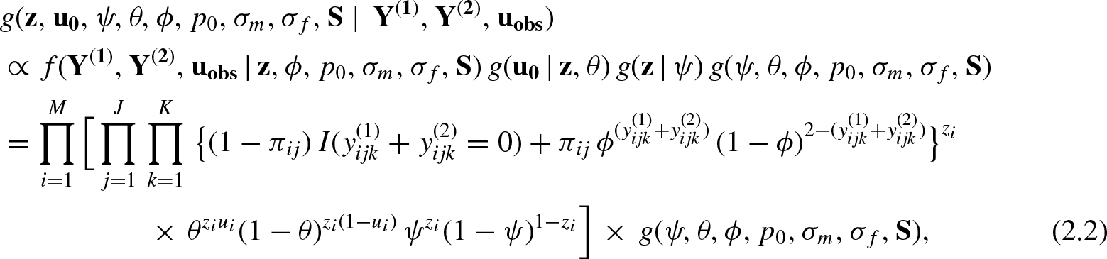
where
Accordingly, the two lists of capture histories generated as in Table 2 essentially come from the same population and therefore there must be a unique association between the two lists. As noted earlier, we are particularly interested to form the associations for the “partially identified” individuals. Accordingly, we treat the true identity of a partially identified individual as a latent variable. We then probabilistically link individuals from the two lists obtained from detector 1 and detector 2, respectively, by introducing a latent identity variable
More details on the synchronization procedure can be found in Royle JA
15
. Without loss of generality, we define the true identity of each individual in the population to be in the row-order of capture histories of detector 1. Then we reorder the rows of detector 2 dataset
An individual i will be called “detected” if there exists a non-zero observation 
where
It is necessary to check for issues of identifiability when new models and estimators such as ours are proposed. Inherent identifiability issues in the model give rise to problems of variance inflation, estimation biases and also false specification of the number of true parameters in penalized methods of model selection.
25
We evaluate the identifiability concerns of two important pairs of parameters in our SECR model,

Note that Equation (2.4) is a four cell multinomial model, where the cells are “00”, “01”, “10” and “11”. This model is identifiable, provided both ϕ and
Link
26
discussed an important and often overlooked aspect of posterior impropriety during Bayesian analysis of estimation problems in ecology and stresses the need for practitioners to ensure that posteriors are proper. More recently, Gopalaswamy and Delampady
27
indirectly suggest the use of defensibly informed or bounded priors to ensure posterior propriety in such problems and indicate the close association between posterior impropriety and identifiability. Accordingly, in this article, we implement bounded priors based on ecologically justifiable upper limits for all the parameters used in our model. The assumed proper prior distributions for these parameters along with other model parameters and latent variables are as follows: a uniform distribution over the interval
Prior robustness is an important issue in Bayesian analysis, and therefore a prior sensitivity analysis is necessary when a fully specified subjective prior is not used. We have indeed performed our computations with the beta prior. Even though there is some information available on the (prior) mean of some of the parameters, the variability is uncertain. Having seen no real differences in the estimates based on a range of beta priors, we have shown only results for the uniform prior, assuming that it is best to report inferences based on a flat prior which is expected to be a robust choice. 28
Use of Covariates
The advantage of the estimator we have developed in this study will only be realized effectively if trap-specific covariates are provided as explanatory variables for the ecological process parameter, p0, as well as observation process parameter, ϕ. In practical wildlife surveys using camera traps, 22 investigators may be interested to assess the movement ecology of animals and assess what factors drive animals to visit particular trap stations or not. For example, investigators might be interested to test the effectiveness of various lures/baits at trap stations or identify local site characteristics that attract or repel animals. These explanatory variables may suitably describe the variation in trap entry probability, p0. However, such covariates are likely to have little influence on whether the cameras installed at trap stations work effectively or not. Instead some other covariates may better describe factors influencing how well the cameras fire and capture records of animals passing by. In real landscapes, heterogeneity in habitat type can induce spatial variation in detection efficiency. For example, detectors placed in regions with high canopy cover may perform more efficiently than detectors placed in open habitats in tropical forests because cooler temperatures under canopy cover enable detection of warm blooded animals better. Similarly, in search-encounter surveys,29, 30 individuals may get differentially detected, spatially, based on the amount of shrub cover. Hence, such covariates can adequately describe the detection probability of the detector, ϕ. It is common practice in ecology, to permit for such covariates in the model using a logit-link for p0 and/or ϕ.
Assessment of Model Performance
Simulation Design
For a high dimensional problem such as this, it would be infeasible to assess model performance for an exhaustive range of parameters simply owing to the number of combinations and computation time. We conducted simulations for 70 scenarios (provided in Appendix Table 1) grouped into 2 equal sized sets, to assess the performance of the model proposed here. We set
Comparison with “Unidentified” Model
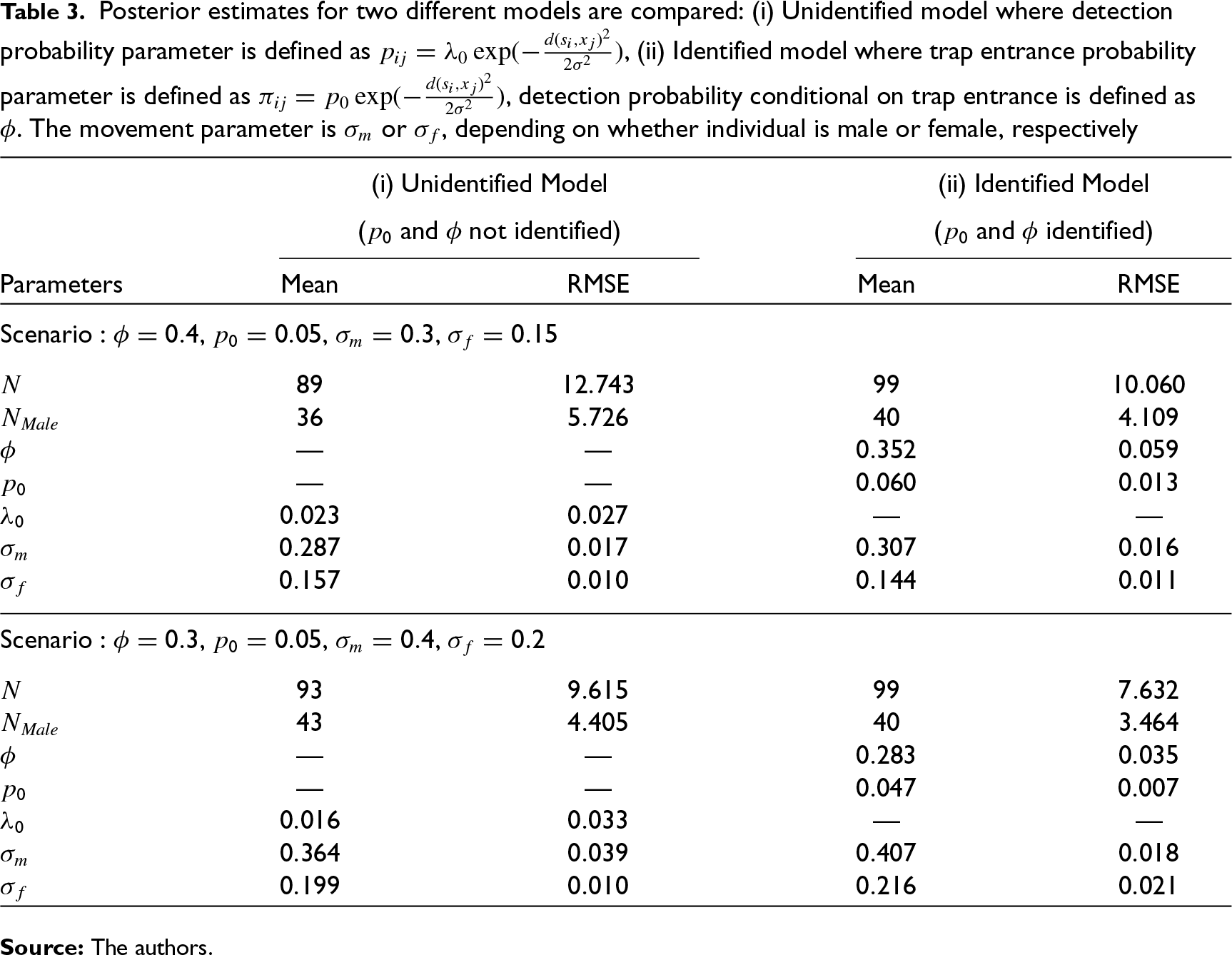
Often practitioners are interested to know about robustness of estimates of particular parameters of interest under violations of model assumptions. For example, ecologists are very interested in N and will often base the choice of their models based on robustness of estimates of N in the face of model violations. Motivated by this concern we also performed a parallel simulation study of the partial identification model proposed by Royle JA 15 . The mechanisms of extracting information from the recorded data sets are different in our proposed model and Royle JA 15 . We view our approach as a natural extension of Royle JA 1 that disentangles the state and the observation processes at the detection region. And is thus not an approach evolved from Augustine et al. 16 Hence, we assess the performance of our model only relative to the more restrictive model. 15 Specifically, we modelled an extra source of variation for the recorded (0,0) events, viz., uncaptured given animal entry in a trap station and uncaptured due to absence of animal in trap station.
Table 3 provides an illustrative example to demonstrate the need for practitioners to use the model we have proposed in this article by indicating the biases in estimates of N and other parameters relative to the reduced, unidentified, model. For ease of comparison we preserve, as before,
Application to Tiger Camera Trapping Data from Nagarahole
Sampling Design
We have considered a specific application of modelling the bilateral capture–recapture data from a single season camera trapping study on tigers in Nagarahole study area of southern India (area = 1,134 km2). The study area extends from 596,626.7 m to 641,533.9 m longitudinally and 1,301,307.5 m to 1,371,205.7 m latitudinally. The coordinates are in Universal Transverse Mercator (UTM) unit system. The trapping array (Appendix Figure 12) consisted of 162 dual camera stations (where two opposite cameras are installed facing each other in each trap station) with a mean spacing of 1.5 km and the survey lasted 50 days (26 November, 2014 to 13 January, 2015), resulting in 7,364 trap nights of effort. We used Panthera branded passive motion sensor cameras (Model: V4, Manufacturer: Panthera) at each trap stations in our study. Usually, the cameras are placed 3–4 m away from the centre of the trail. This setup ensures that each camera can clearly obtain independent flank images. 14
Our use of the Gaussian function implies that the buffer around the trapping array should, theoretically, be set at infinity. However, for practical reasons, this is usually set large enough so that individuals have a near zero probability of being exposed to the trapping array beyond such a buffer.
13
Accordingly, we set a buffer of 10 km (aiming for a width
Tigers can be individually identified by matching the unique patterns of flanks on both left and right sides. Researchers use software 32 to assist in matching flank patterns from photographs and consequently obtain individual specific detection histories in standard spatial capture–recapture format. 13 However, since flank patterns are not identical on both sides of a tiger, at least one simultaneous detection of both side flanks over the course of camera trapping survey is needed to identify a tiger. A “simultaneous detection” is defined for an individual when the event time recorded by passive motion sensor cameras matches exactly (to the minute) for either flanks of an individual. Data were arranged in the format described by the sampling structure defined in Table 2.
Data Summary
In our field experiment, we could identify 65 tigers (22 male, 33 female, 10 of unknown sex). This meant that we recorded at least one simultaneous capture of both flanks for each of the above set of tigers. In addition, we obtained 14 partially identified left flank only detection histories (6 male, 5 female, 3 of unknown sex) and 17 partially identified right flank detection histories (7 male, 4 female, 6 of unknown sex). Overall, we obtained 123 simultaneous detections, 126 left flank only detections and 137 right flank only detections.
Analysis
We used the covariate information on sexes for the detected individuals. As male and female tigers do not share the same σ, that is, do not have the same home-range size, we modelled σ as a function of this covariate. We fitted the model described in Section 2.2.1 and augmented the detection histories by all-zero detections to make them of the same dimension. We ran one chain of 50,000 iterations and discarded first 25,000 as burn-in. Further, we assessed the quality of the parameter estimates by computing the coverage probabilities. Here, we fixed the parameters at the values estimated in the data analysis and simulated 100 data sets under the same conditions (i.e., state space, trap deployment) as in the case of the Nagarahole study. Coverage probabilities are computed as the proportion of times when the estimated 95 per cent CIs contain the true value of the parameter. In these simulations, the true values are defined as the posterior mean estimates from the results of the field experiment of the following parameters: N,
Results and Conclusions
Assessment of Model Performance
Simulation Results
Here we summarize the main findings of the simulation study over different simulation scenarios as mentioned in Section 2.3.1. The detailed discussion of the study is provided in Appendix C and the simulation results are presented in Appendix Tables 3–10. We observe that, the quality of the estimates of different parameters substantially improves when trap entry probability p0 increases. The scenarios in which p0 is set to values greater than 0.03 had performed reasonably well. This is noted by the manner in which root mean square error (RMSE) values shrink substantially as p0 increases. Whereas when the trap entry probability p0 is set at low values (below 0.01), in most of those scenarios the posterior estimates of parameters are inaccurate with wide 95 per cent CIs. This outcome may be explained by the poor information content emerging when individuals rarely enter trap stations. The boxplots (Appendix Figure 2) of N, obtained by using the MCMC samples, show signs of positive skewness in most of the scenarios. Also, the bias and posterior standard deviation (SD) of N are influenced by the conditional detection probability ϕ (indicating detector performance) in a similar manner to how p0 influences model performance. That is, both bias and posterior SD decrease as the value of ϕ increases.
The scenarios with
The posterior mean estimates of p0 have a decreasing trend on bias as ϕ increases. In a similar manner, posterior mean estimates of ϕ also have a decreasing trend on bias as p0 increases. This simulation outcome is indicative of poor information content in the data and consequently reflects on the identifiability of the parameter estimates. We surmise that these correlations will play an important role during model selection and inference.
Comparison with “Unidentified” Model
In both the scenarios,
Posterior estimates for two different models are compared: (i) Unidentified model where detection probability parameter is defined as
, (ii) Identified model where trap entrance probability parameter is defined as
, detection probability conditional on trap entrance is defined as ϕ. The movement parameter is
or
, depending on whether individual is male or female, respectively
Data Analysis
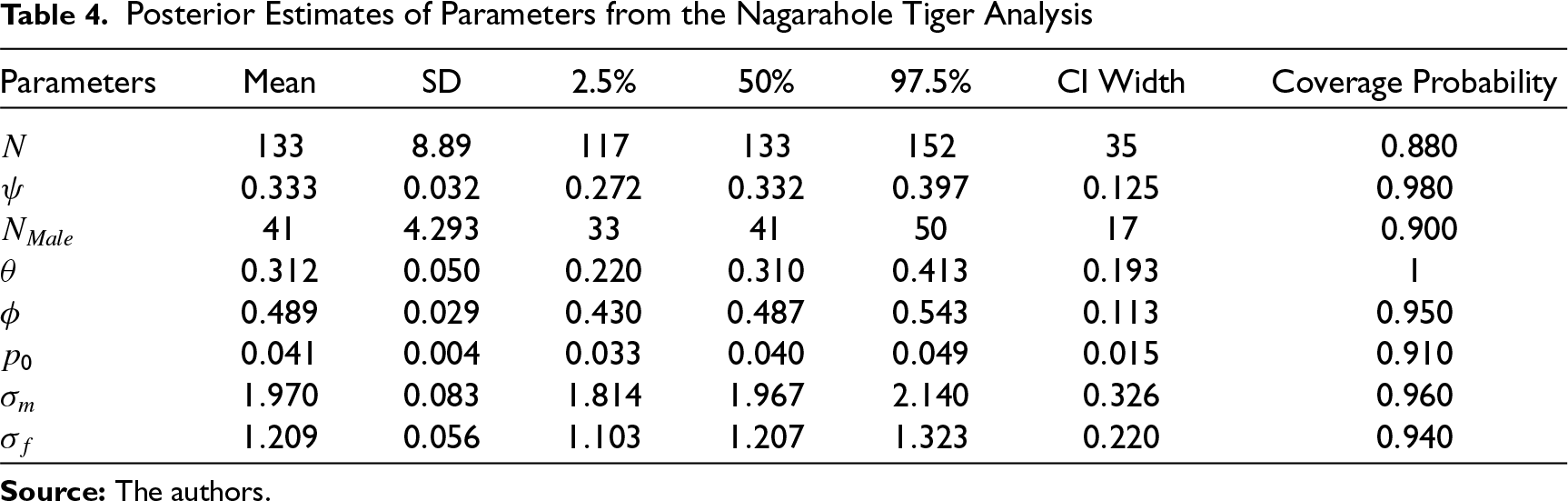
The posterior estimates of parameters are provided in Table 4. The posterior mean estimate of population size (over the state space) is 133 with a 95 per cent CI of (117, 152). The density of tiger is estimated at 11.73 tigers per 100 km
2
in our study area. The posterior mean of
The scatter plot provided in Appendix Figure 15 shows that there is moderate amount of correlation between ϕ and p0 (
Inference
The detection probability ϕ in the analysis of Nagarahole capture–recapture dataset on tigers is estimated at 0.489 (see Table 4). This implies that each camera records a clear flank image in a little less than 50 per cent of the cases. This is not surprising to us as a clear “valid sample” depends on many other factors, such as quality of the traps, camera malfunctions, ambient temperature etc. in typical field conditions.
The simulation study was designed to reflect a typical field study, so that performance of the model can be evaluated based on different values taken by the model parameters in a practical setup. Accordingly, p0 is the most dominant parameter which influences the performance of the model while obtaining posterior summaries of the other parameters. Furthermore, the estimates corresponding to the scenarios where p0 is set to 0.05 or 0.07 perform fairly well as compared to the scenarios where p0 is set to smaller values, viz., 0.005, 0.01. In the field study p0 is estimated at 0.041 with a 95 per cent CI (10.32, 13.41) (see Table 4).
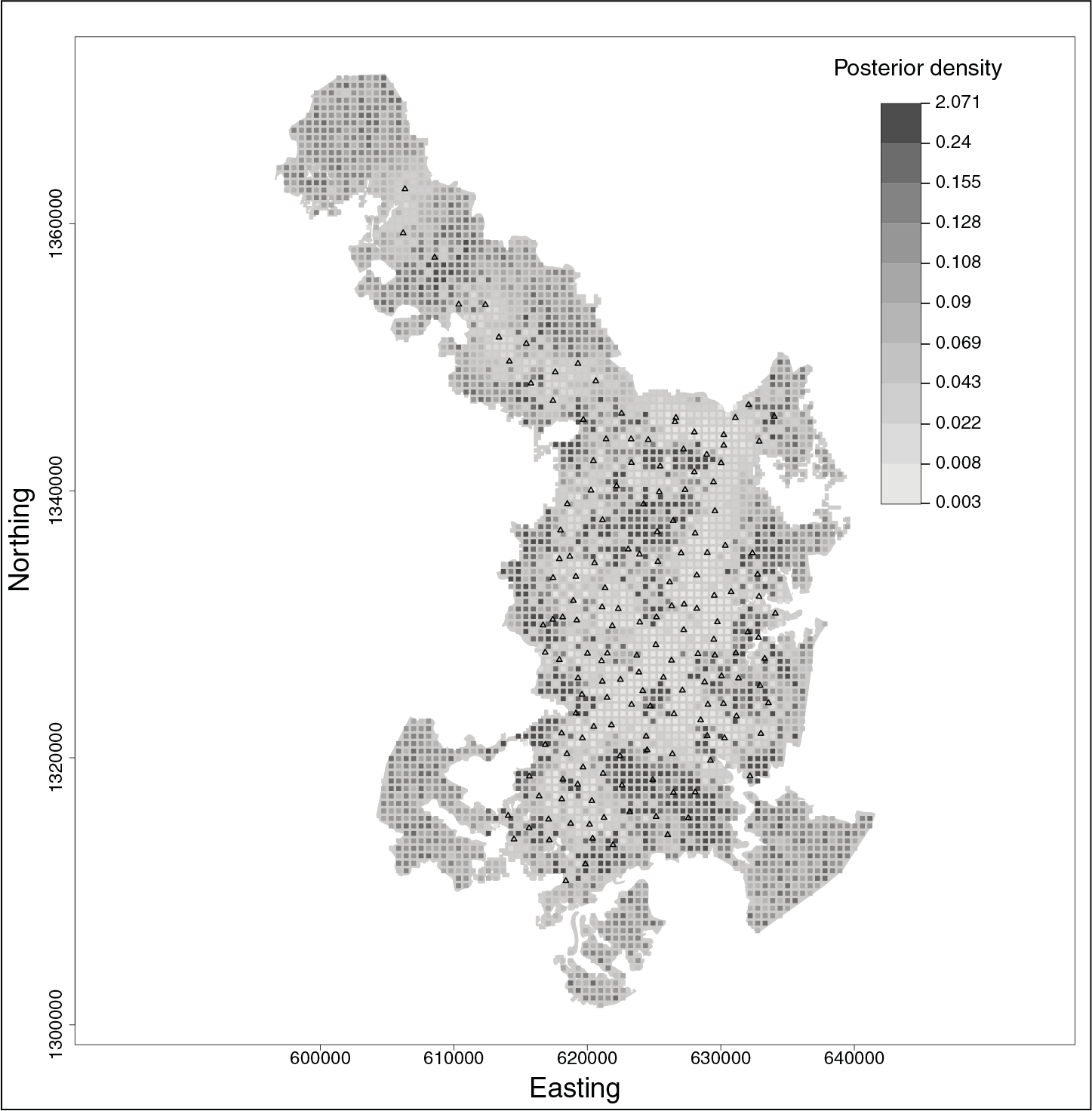
We estimated the tiger density to be 11.73 tigers per 100 km2 with 95 per cent CI (10.32, 13.41) in our study area. This is comparable to estimates of tiger density from a similar study 21 in this area using a different version of SECR models. The 95 per cent CI width of 3.09 from our study is only 26.3 per cent of its corresponding density estimate. In comparison 21 , had 95 per cent CI widths as 42.5 per cent of their density estimate (11.3 tigers per 100 km2 with 95% CI [9.1, 13.9]). Clearly our model provides more precise estimates for tiger density. The estimated posterior density map of tigers (per sq. km.) over the study area is provided in Figure 1.
We found that coverage probabilities of all the continuous parameters (viz.,
Posterior Estimates of Parameters from the Nagarahole Tiger Analysis
Posterior Estimates of Parameters from the Nagarahole Tiger Analysis
In this article, we have developed a novel SECR estimator that successfully disentangles the ecological process of animal trap entry from the observation process of trap detection rates (see Section 2). Our simulation results highlight the relative importance of ensuring that trap stations are chosen based on good locations as compared to the importance of detector choice, especially, when there is more than one detector located at each station. When adequate spatial coverage is achieved by the array of detectors, as per the recommendation by Karanth and Nichols 14 , it is preferred that good spots are to be selected locally to maximize the probability of animal arrival.
Our SECR model is built upon an earlier Bayesian hierarchical model by Royle JA 15 and makes full use of all data available (including information on partially identified individuals). We demonstrate how our model provides unbiased estimates of population size N when trap detection rate is less than one. We justify the importance of estimating trap detection rate ϕ by showing the bias in the estimate of N when we use the Royle JA 15 model under certain simulation conditions.
We have developed the estimator using the special case of having only two detectors at each station, each detector capturing a set of unique traits about the identities of individuals. The assumption, however, is that each detector contains enough information on its own to ascertain individual identity. For example, as this study was motivated by the tiger example we have discussed in the article, we find a field situation where two profile flanks of an individual tiger are attempted to be caught at the same time at trap stations. When we do not have simultaneous captures it is not possible to tell if a right flank image of a tiger has an equivalent left flank image or not. We recognize that the situation will not directly apply if the same idea is extended to genotyping problems34, 35 because at each locus there is not enough information to convincingly identify individuals. We discuss more on this application later.
It is possible to extend our model to include three or more detectors per station based on the idea of how occupancy models 36 were constructed to include multiple sampling occasions. However, we envisage some complications with regard to explicitly defining the permutative arrangement of capture histories. For this, we need to understand how many detectors (implying how many sets of unique features) are necessary to establish full identity of an individual. For example, in genotyping problems 35 , workers identify a panel of loci to achieve a desirably low level of probability of identity (PID). During field surveys34, 37, workers often gather faecal samples for subsequent genotyping. However, not all faecal samples amplify in the laboratory. We envisage the application of our model to estimate this probability using the parameter ϕ.
As with most estimators, the utility of our SECR model is enhanced when meaningful covariates are applied on the specific model parameters. Ecologists interested in obtaining an understanding about fine scale movements of animals can now do so without the worry about the confounding problem of detector efficiency. We envisage that our estimator will find much use in optimal allocation problems 16 in wildlife surveys. For example, many camera traps are available in the market at various costs. Since our model specifically estimates a parameter ϕ associated with trap efficiency, it would come of use to evaluate the relative gains in precision of estimates of abundance when, for example, cheap cameras are replaced by expensive cameras or to decide how many traps are needed at each station. Further, for defined monitoring budgets our model can be used to determine the most optimal allocation of the number of trap stations and the types of traps with available resources.
Beyond ecology, our SECR estimator lays the foundation for solving the statistical reconciliation problem in administrative lists. 38 In this problem, individuals do appear in different administrative lists at a region and the problem is to identify the population size from captures of individuals in the multiple lists. We find equivalence between multiple detectors discussed in our problem with the presence of different administrative lists in the problem described by Madigon and York. 38
An inherent problem in the application of a complex model for real world problems, and a larger problem in the statistical literature, is that selecting the appropriate model for prediction and characterization of populations is not straightforward. Some of us are currently working on evaluating and applying various model selection tools on this class of Bayesian SECR problems. We also encourage the extension of this estimator to include multiple detectors (more than two) as described above. With these developments, we envision wide application of the general approach presented here.
Supplemental Material
bilateral_supp_010119_highlighted_xyz13726f955f904 - Supplemental material for A Spatially Explicit Capture–Recapture Model for Partially Identified Individuals When Trap Detection Rate Is Less than One
Supplemental material, bilateral_supp_010119_highlighted_xyz13726f955f904 for A Spatially Explicit Capture–Recapture Model for Partially Identified Individuals When Trap Detection Rate Is Less than One by Soumen Dey, Mohan Delampady, K. Ullas Karanth, Arjun M. Gopalaswamy in Calcutta Statistical Association Bulletin
Footnotes
Acknowledgements
We thank the anonymous reviewers for some very useful comments and suggestions, which have brought improvements to our presentation. We thank the Indian Statistical Institute for financial and administrative support and the Centre for Wildlife Studies and Wildlife Conservation Society, New York for providing the data and analytical support. We also thank Ravishankar Parameshwaran and Devcharan Jathanna for help with the computer simulations and helpful advice. AMG thanks the Wildlife Conservation Society, New York for partial funding support.
Declaration of Conflicting Interests
The authors declared no potential conflicts of interest with respect to the research, authorship and/or publication of this article.
Funding
The authors received no financial support for the research, authorship and/or publication of this article.
Supplementary Materials
Supplemental material for this article is available online.