
Abstract
This article proposes two estimators for two semiparametric count regression models, namely semiparametric partially Poisson (SPPO) and semiparametric partially zero-inflated Poisson (SPZIP), via the penalized smoothing (Ps) spline and P-spline (Pb) estimations to address the common issue of nonparametric relationships between the response variable and covariates. Additionally, the SPZIP model incorporates a zero-inflation component to handle excess zeros in count data. Through extensive Monte Carlo simulations, we rigorously evaluate the performance of the proposed penalized spline estimators by comparing them against traditional parametric estimators using multiple statistical criteria, including the Akaike information criterion, Bayesian information criterion, deviance statistic, mean squared error and root mean squared error (RMSE). The results indicate that our estimators are more efficient than other estimators. Also, the SPZIP and SPPO models consistently outperform parametric (Poisson and zero-inflated Poisson) regression models, particularly in scenarios with high levels of zero inflation, demonstrating their superior ability to model complex data structures. Our findings highlight the practical utility of these models for analyzing complex count data with excess zeros and nonparametric covariate effects. A real-life data application further demonstrates the capabilities of the SPPO and SPZIP models, demonstrating their ability to provide more accurate and adaptable statistical analysis in challenging data settings.
Introduction
A model is just a simplified representation of reality or the real-world. Generally, models are classified as deterministic or probabilistic. The models used to examine the functional relationship between dependent variables and independent variables are known as regression models and can be classified into three types, which are parametric, nonparametric, and semiparametric regression models. The regression function represents this functional relationship. So, if the regression function is known, it produces a notable model known as the parametric regression model. If this relationship is unknown, it produces a regression model known as a non-parametric regression model. The combination of parametric regression models and nonparametric regression models produces semiparametric regression models. This means that this model is used in cases where the parametric assumptions are not met or the non-parametric model is not the most efficient.
One of the most popular parametric regression models is the linear model, which is used when the response variable follows a normal distribution. This model is predicated on several assumptions and a set of finite parameters, β. Since the response variable does not always follow a normal distribution, the linear model is not applicable in many practical scenarios or real-life applications. For instance, response variables may occasionally be measured on a count, binary, ordinal, non-negative scale or other limitations. Nelder and Wedderburn[1] presented the concept of generalized linear models (GLMs) as a way to get around these problems. Thus, GLMs are extensions of the linear model under these limitations, provided that the response variable distribution is a member of the exponential family of distributions and that it is also a parametric regression model. In the case of parametric regression models, the count regression models with the problem of excess zeros are considered one of the most common GLMs due to their use in many fields, such as insurance, public health, epidemiology and psychology. For instance, Abonazel et al., [2] Algamal et al., [3] Akram et al., [4] Dikheel and Jouda,[5] Abdelwahab et al., [6] Zeeshan et al.[7] and Shahsavari et al.[8]
In recent years, there has been considerable interest in semiparametric regression models, which have a long history in statistics. The main reason they are considered is that sometimes the relationships between the response and explanatory variables are very heterogeneous within the same model because some of the relationships are linear, while others are more complex to classify. More explicitly, some variables are parametrically related, while others are nonparametrically related. Numerous semiparametric regression models exist, including the partially linear model (PLM), a significant generalization of the linear model that permits the majority of predictors to be modelled linearly while one enters the model nonparametrically and is a special case of the additive model. The generalized partial linear model (GPLM), one of the most popular semiparametric regression models, extends the PLM when the dependent variable follows any distribution within the exponential family except the normal distribution. In another sense, GPLMs are an extension of the GLMs by blending nonparametric models for some covariates. The GPLM has been applied in several areas of knowledge, such as toxicology, biology, sciences and statistics.
Recently, some literature has reviewed estimation and inference methods for the GPLM, which can handle both linear and nonlinear relationships simultaneously. For example, Green and Yandell [9] introduced the semiparametric GLM in which they added a nonparametric component to the linear predictor. Carroll et al.[10] extended semiparametric GLMs to partially linear single-index models, enabling the modelling of intricate relationships. They also developed backfitting algorithms for estimation. Härdle et al.[11] introduced kernel-based methods for estimating semiparametric GLMs and provided statistical tests for model selection. Wood [12] applied semiparametric Poisson (PO) regression to model daily deaths in Chicago, demonstrating the practical use of these models. Additionally, they provided a comprehensive introduction to generalized additive models, a special case of semiparametric GLMs, using R dataset, Lam et al.[13] developed a semiparametric zero-inflated Poisson (ZIP) regression model using sieve maximum likelihood and B-splines to address the challenges of excess zeros in count data. Liang et al.[14] studied semiparametric GLMs for longitudinal data and proposed an empirical likelihood-based inference method for GPLMs, providing a robust and efficient approach to statistical inference. Taylan et al.[15] applied semiparametric GLMs to analyse survival data and focused on the theoretical foundations of parameter estimation for GPLMs, specifically using B-splines and continuous optimization techniques. De Vera[16] introduced the semiparametric PO regression model; the parametric and nonparametric components in this model were estimated by penalized maximum likelihood and backfitting algorithm. Manalaysay and Barrios[17] presented a similar work where they focused on the principal component of the PO regression model, and the model is estimated via the backfitting algorithm. Yousof and Gad[18] introduced a robust Bayesian framework for estimating and conducting inference within GPLMs, effectively integrating linear and nonlinear components to capture complex relationships in data. They focused on Bayesian estimation and inference of the model parameters using multivariate conjugate prior distributions under the square error loss function. For more details about prior and posterior distributions, see the studies of Seliem et al.[19] For more details, the studies of Müller,[20] Luts and Wand,[21] Lukusa et al., [22] Fang et al.,[23] Wurm and Rathouz,[24] Ye et al.[24] Boente et al.[25] and Boente et al.[26] can also be reviewed.
Rahman et al.[27] proposed efficient inference methods for GPLMs, a class of models that flexibly accommodate linear and nonlinear relationships. Their novel estimation approach achieves semiparametric efficiency, enhancing statistical accuracy. El-sayed et al.[28] demonstrated the effectiveness of a novel B-spline Speckman estimator for PLMs. Their results showed improved performance compared to traditional methods, highlighting the advantages of using B-splines to estimate the nonparametric component. Abonazel and Gad[29] introduced a robust partial residual estimation approach for semiparametric PLMs. Their results showed that this method outperforms traditional techniques, particularly in settings affected by outliers. For additional discussions on outlier treatment in different models, see, for example, Abonazel and Gad,[29] Seliem,[30] and Soliman et al.[31]. Meanwhile, Ibacache-Pulgar et al.[32] proposed the semiparametric zero-inflated negative binomial (ZINB) model, which extends the standard ZINB framework. Similarly, Araújo et al.[33] examined determinants of academic performance among undergraduate business students, focusing on the number of failed courses. To analyse their data, they applied a semiparametric ZINB regression model, incorporating factors, such as employment status, dissatisfaction with affirmative action scholarships and the challenges of combining work with study. For more details, the studies of Shao and Wang,[34] Prataviera et al., [35] Millard and Kanfer,[36] Vasconcelos et al., [37] Cardozo et al.[38] and Vasconcelos et al.[39] can also be reviewed. To overcome the difficulties of evaluating proportional data with excessive zeros and intricate correlations, Seliem et al.[40] suggested an innovative semiparametric zero-inflated Beta (SPZIBE) regression model via penalized smoothing (Ps) spline and P-spline (Pb) estimators. By accounting for both linear and nonlinear effects, this model provides a versatile and interpretable method that makes it possible to identify the elements causing zero inflation. The authors demonstrated the model’s superior performance through extensive simulations and real-life applications, showcasing its potential to outperform existing parametric models in terms of model fit and predictive accuracy. This research significantly contributes to the field of statistical modelling by providing a valuable tool for analysing various types of data, including those encountered in political science, economics, and social sciences. This work aims to discuss the semiparametric partially Poisson (SPPO) and the semiparametric partially zero-inflated Poisson (SPZIP) regression models and propose two estimators using the Pb and Ps estimators to estimate the nonlinear effects of covariates.
The structure of this article is as follows: the parametric regression models, the PO regression model and the ZIP regression model, are briefly described in
Methodology
This section aims to present the PO and ZIP regression models and the maximum likelihood estimator (MLE) for both models.
PO Regression Model
Regression model analysis is considered one of the most powerful techniques used to study the relationship between two or more variables in various fields and is widely used for both prediction and interpretation purposes. Consider another regression modelling scenario where the response variable of interest is not normally distributed. In this situation, the response variable represents the count of some relatively rare events. The simplest probability distribution for count data is the PO; the distribution is skewed to the right with restriction ‘variance equal to the mean’. So, the PO regression model is not a safe strategy when data show over- or under-dispersion. In a broader sense, the cases in which the PO regression model is appropriate are when the response variable is an observed count, which follows the PO distribution since the response variable’s values are non-negative integers. The regression coefficients in the PO regression model are estimated using the MLE. Since the PO distribution is a member of the exponential family. So, the density function of the exponential family is defined as
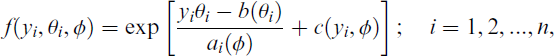
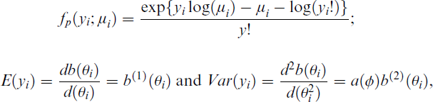
where, in each case, a(·), b(·) and c(·) are specific functions; the function ai(ϕ) has the form ai(ϕ) = ϕpi, where pi is a known prior weight, usually 1, θ represents the link function and is called the canonical parameter, which is a function of the mean (μ) of the distribution, b(θ) is a function of the canonical parameter or the cumulant, which is also a function of the mean because θ is a function of mean, ϕ is a dispersion parameter that plays a role in defining the variance of y and c(yi, ϕ) is a function of observation y and the dispersion or scale parameter ϕ and indicates the normalization term. Assume that the counts, yi(i = 1, 2, …, n), are produced independently using the PO distribution, where the probability mass function (p.m.f.) of the response variable is provided by

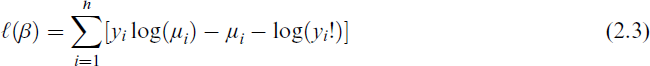
Equation (2.1) can be rewritten in exponential family form as follows:
where b(1) and b(2) refer to the first and second derivatives

where
To estimate the unknown regression parameters of the PO regression model, the most popular approach is the MLE. For the canonical link, we have

where

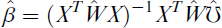
Iterative techniques are used to acquire the solution since Equation (2.4) is nonlinear in β. The iteratively re-weighted least squares (IRLS) method is a popular example of such a process. With r iterations, let βr be the estimated value of MLE of β. This can be expressed as

where
and
As discussed above, the PO regression model assumes that the response variable’s conditional mean and conditional variance are equal, and violating this condition leads to the problem of excess zeroes. Hence, the PO regression model is not suitable for representing the data in the presence of this problem. Consequently, the zero-inflated regression models are the best models to represent these data. Zero-inflated regression models are statistical models specifically designed for counting data with excess zeros. They essentially model the data in two parts: one process explains ‘true zeros’ and another explains ‘excess zeros’. A common example of these models is the ZIP model. The ZIP model is a mixture of two distributions. The zeros are assumed to arise from two different states, the first is a degenerate distribution at zero (i.e., zero inflation) that occurs with probability π and produces structural zeros, while the second is a PO distribution that occurs with probability 1 – πi and is called sampling zeros, which occur by chance. The parametric ZIP can, then, be formulated as follows:
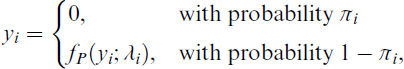
where yi is a response variable, and fp(yi, λ) set the space here denotes PO distribution with parameter λi > 0. Hence, if πi = 0, the ZIP model reduces to a PO distribution, as in Equation (2.5). More clearly, the ZIP model can be presented as follows:
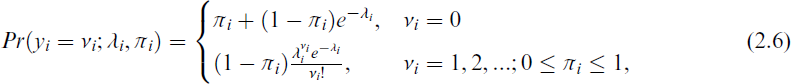
where λi is the PO mean corresponding to the susceptible population for the ith individual (i = 1, …, n), and πi is the probability of belonging to the nonsusceptible population. For the ZIP distribution, the mean and variance are as follows:

To use the parametric ZIP model with covariates, Lambert[41] suggested the following joint models for λ and π:

where

where I[△] is the indicator function of the set △. Substituting Equation (2.7) into Equation (2.8) yields

Iterative techniques are used to acquire the solution because Equation (2.9) is nonlinear in ω. IRLS or expectation-maximization algorithms are examples of such procedures that are frequently used.[43]
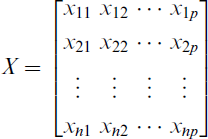
This article develops estimation for two semiparametric count regression models: the SPPO regression model and the SPZIP regression model. The proposed estimation framework utilizes Ps spline and Pb approaches to capture potential nonparametric covariate effects. While both models address nonparametric relationships, the SPZIP regression model incorporates a zero-inflation component to handle excess zeros in count data. The semiparametric models offer more flexibility than their parametric counterparts by relaxing strict distributional assumptions. Many real-life phenomena exhibit response variables that do not follow a normal distribution. When parametric models are insufficient to describe the relationship between dependent and independent variables, semiparametric regression models provide a more flexible alternative. For example, the GPLM assumes that the conditional expectation of the response variables, given the covariates, can be represented as

where the explanatory variables are split into two vectors: X, an n × p design matrix of parametric covariates, and T, a q-variate random vector of continuous covariates that enter the model nonparametrically, β is a p × 1 vector of finite-dimensional unknown parameters, σ2 is the dispersion parameter and m(·) is an unknown smooth function estimated nonparametrically. The model in Equation (3.1) assumes a linear relationship between the response variable and X and a nonlinear relationship with T. Here, G(·) : R → R is a known link function, chosen based on the range of the response variable. Several approaches can be used to estimate the nonparametric component in semiparametric regression models, including kernel smoothing, local polynomial regression and cubic spline. By combining parametric and nonparametric components, GPLMs offer more flexibility than traditional GLMs. However, this increased flexibility comes with additional complexity and computational challenges.
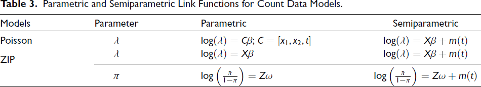
In some cases, we need to extend the parametric PO regression model with the link function in Equation (2.2) into a SPPO regression model with a partially linear link function or a broader systematic component for λ as follows:

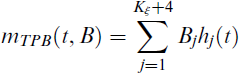
where m(·) is a smoothing function related to the continuous explanatory variable with the nonlinear effect that is controlled nonparametrically. The SPPO regression model can be seen as a generalization of the PO regression model presented in Equations (2.1) and (2.2) by including a nonparametric function. Then, Equations (2.1) and (3.2) define the SPPO regression model to represent linear and nonlinear effects jointly. Regarding the nonparametric component, m(·), in Equation (3.2), there are several approaches to estimate it, including cubic smoothing spline, B-spline and truncated power basis (TPB).[44] For example, the smooth function m(·) is approximated by the TPB, mTPB(t, B). The equation for a spline of degree d with Kξ knots is given by
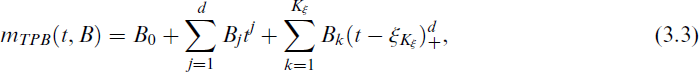
where
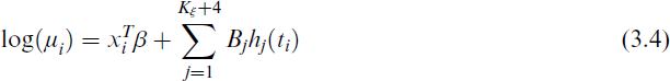
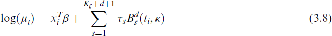
Therefore, the PO mean log(μ) in Equation (3.2) can be expressed as
Another example, the smooth function m(t) is approximated by a spline function mBS(t, κ) that can be expressed as a linear combination of the B-spline basis functions as follows:
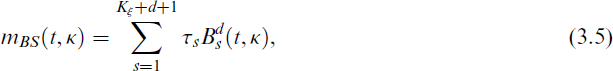
where τs are unknown regression coefficients, s = 1, …, Kξ + d + 1, and Bd(t, κ) are the B-spline functions and can be expressed as follows: let ξ0 = Ψ and
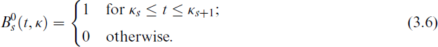
Where

Note that additional 2d + 2 knots are necessary to build the full B-spline of degree d. Briefly, a complete B-spline matrix of degree d for n observations based on Kξ knots has dimension n × (Kξ + d + 1). The total number of knots for the construction of the B-spline will be Kξ + 2d + 1. Then, the number of B-splines in the regression is equal Kξ + d + 1, for more details see the work of Goepp et al.[45] Therefore, the PO mean log(μ) in Equation (3.2) according to the B-spline regression can be expressed as
Let (Ψ, Ω) be an interval and let

where
The concept of Ps splines was originally introduced by O’Sullivan.[46] However, Eilers and Marx[47] pioneered the use of B-splines with different penalties, a technique now known as Pbs. Pbs combine regression on B-splines with a discrete roughness penalty to smooth scatterplots. B-splines are constructed from polynomial pieces joined at specific points called knots. Once the knots are defined, B-splines of any desired degree can be computed recursively. The penalty term for Equation (3.9) can be written as follows:

where Ms is a positive semidefinite penalty matrix that is
s
×
s
. [28] However, Eilers and Marx[48] showed that the integrated square of the kth derivative of m(t) is well approximated by a penalty on finite differences of the coefficients Υ
s
with much less effort, that is,

where

Thus, we have that β and m are estimated by maximizing the logarithm of the penalized likelihood function in Equation (3.12). Regarding the banded matrix, Dk can be computed recursively, where D1 has dimension (n − 1) × n, with ki, i = 1, ki, i +1 = 1 and all other elements are 0, mostly k = 2 or k = 3 is used. The penalized splines technique employs fewer knots while demonstrating greater robustness to knot placement compared to traditional smoothing splines.[45, 49] The generalized additive models for location, scale and shape (GAMLSS) package enhances this approach through automatic knot selection, effectively balancing model complexity and efficiency. While Ruppert et al.[49] recommended maintaining 4–5 observations between knots, large datasets benefit from an upper limit of 20–40 knots[50] to ensure computational efficiency.
Consider a semiparametric link function for λ, the partly linear link function is one possibility giving the joint models with

The Generated Variables Under Different Scenarios.
where t is an observable continuous covariate, and m(·) is an unknown smooth function related to continuous covariates with nonlinear effect that is modelled nonparametrically. The model specified by Equations (2.6) and (2.7) is an extension of the class of generalized linear mixed models, while the model specified by Equations (2.6) and (3.13) is an extension of the class of generalized partially linear mixed models by incorporating a nonparametric component, m(t), alongside parametric terms. Let 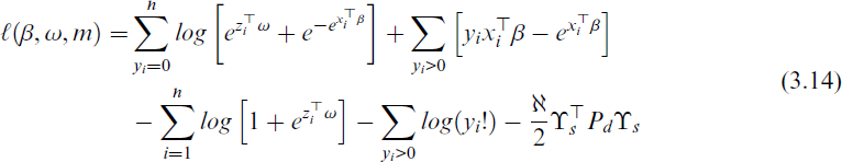
This semiparametric penalized log-likelihood function incorporates fixed-effects parameter vectors β ∈ Rp and ω ∈ Rq for the count and zero-inflation components, respectively, and a nonparametric smooth function m(·) to model nonlinear covariate effects, where its smoothness is enforced by the penalty term
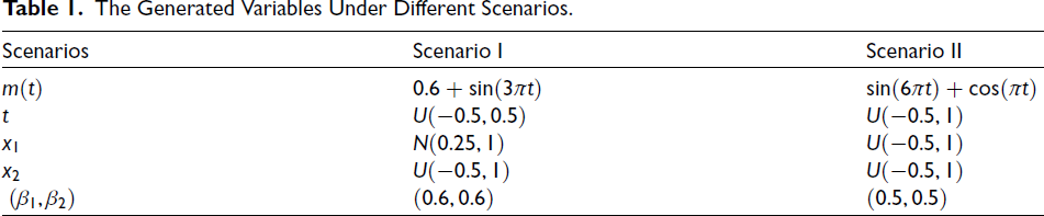
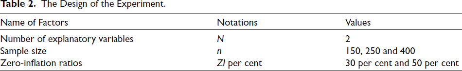
To assess the performance of parametric and semiparametric PO and ZIP models, a Monte Carlo simulation study was conducted. The nonparametric part was performed via Ps and Pb estimators, specifically the SPPO and SPZIP with (Ps and Pb) estimators. The R software with the GAMLSS package was employed to simulate data under various scenarios, including sample sizes of 150, 250 and 400 and zero-inflation levels of 30 per cent and 50 per cent as in Table 2. For each scenario, 1,000 datasets were generated, with the response variable yi following ZIP(λ, π) distribution and covariates (x1, x2), and t specified as in Table 1.
The Design of the Experiment.
The Design of the Experiment.
Parametric and Semiparametric Link Functions for Count Data Models.
Additionally, we explored the use of sine–cosine functions for the nonparametric component, as outlined in Table 1. Furthermore, following the work of Rahman et al., [27] alternative nonparametric functions can be considered for future research. The deviance statistic (DVS), mean squared error (MSE), Akaike information criterion (AIC) and Bayesian information criterion (BIC) were used to assess each model’s performance. Average estimates (AEs), MSE and root mean squared error (RMSE) were used to evaluate the goodness-of-fit of the estimated parameters 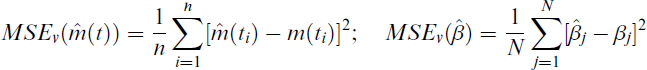
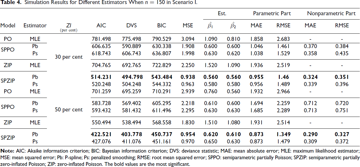
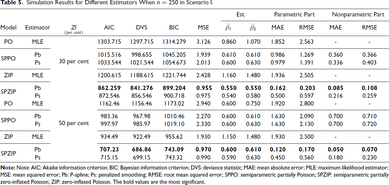
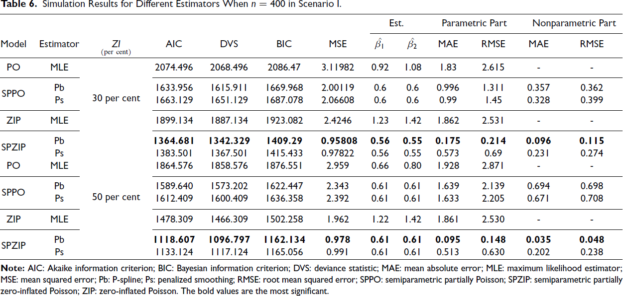
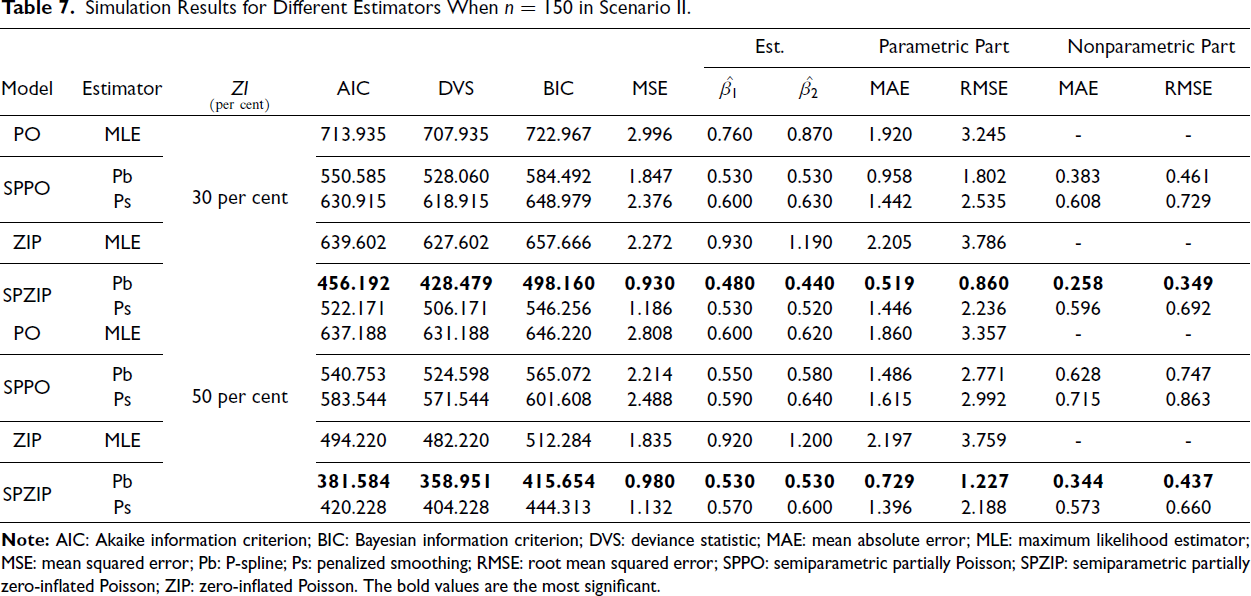
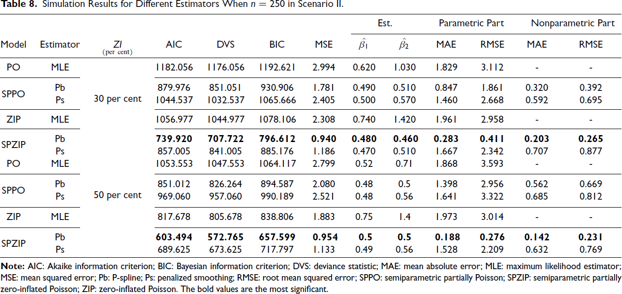
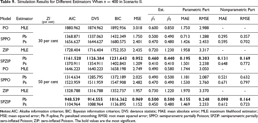
Zero-inflated count data pose significant challenges in statistical modelling due to the excess zeros. To address this issue, we evaluated the performance of various count models, including parametric, PO and ZIP, and semiparametric, SPPO and SPZIP. Simulated data were generated under different scenarios with varying levels of zero inflation and sample size as in Table 3. The models were fitted to these data and evaluated using multiple criteria, including AIC, BIC, DVS, MSE, mean absolute error (MAE) and RMSE. Lower values of these metrics indicate better model fit.
Our findings consistently demonstrate the superior performance of the SPZIP regression model, particularly when using the Pb estimator (ZIP.pb). This model achieved the lowest values for all evaluation metrics, including AIC, BIC and MSE, and exhibited enhanced performance with larger sample sizes and higher levels of zero inflation. The SPZIP model’s flexibility in capturing both parametric and nonparametric components of zero-inflated count data enables more precise parameter estimation and improved model fit, especially in complex data structures. As shown in Tables 4–9, the SPZIP regression model with the Pb estimator consistently outperformed traditional parametric methods, reinforcing its position as a robust and effective statistical tool for analysing zero-inflated count data.
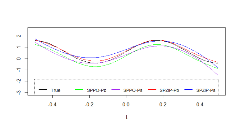
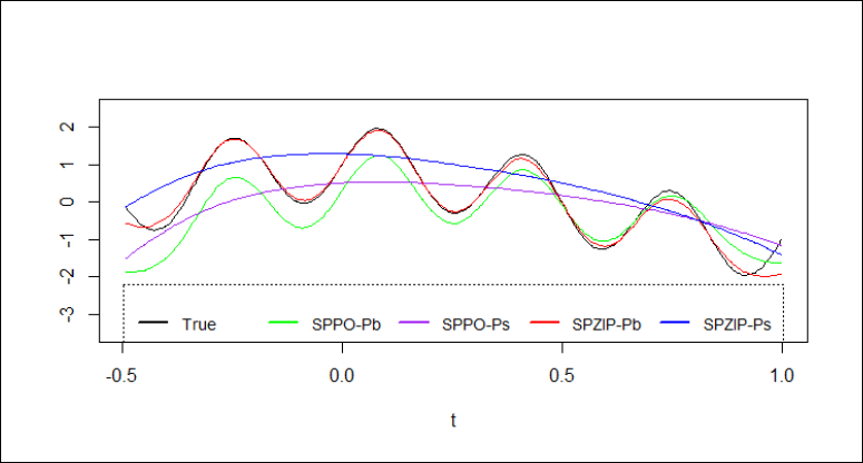
Figures 1 and 2 provide a clear visual comparison of the fitted values for the estimators of m(t) under different scenarios (n = 400, ZI = 30 per cent and 50 per cent). The SPZIP regression model consistently demonstrates the closest alignment with the true function across both scenarios, specifically the SPZIP with Pb estimator. This visual evidence corroborates the findings from the evaluation metrics and further solidifies the superior performance of the SPZIP regression model in capturing the complex nonparametric structure of the data. The analysis shows that the SPZIP regression model outperforms other models in several key aspects that can be summarized as follows:
Simulation Results for Different Estimators When n = 150 in Scenario I.
Simulation Results for Different Estimators When n = 250 in Scenario I.
Simulation Results for Different Estimators When n = 400 in Scenario I.
Simulation Results for Different Estimators When n = 150 in Scenario II.
Simulation Results for Different Estimators When n = 250 in Scenario II.
Simulation Results for Different Estimators When n = 400 in Scenario II.
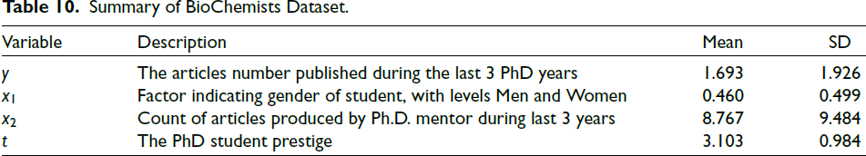
Summary of BioChemists Dataset.
In this section, we present a real-life application to evaluate the effectiveness of proposed estimators.
BioChemists Dataset
This section demonstrates the applicability of the SPZIP regression model through comparative analysis using real-life data. We utilize the biochemistry graduate students’ dataset (bioChemists) from R software, previously analysed by Al-Taweel and Algamal,[51] to compare parametric regression models (PO and ZIP) with their semiparametric counterparts (SPPO and SPZIP). The semiparametric models incorporate a nonparametric component estimated using the Ps and Pb estimators. The dataset comprises 915 observations, with basic statistics reported in Table 10.
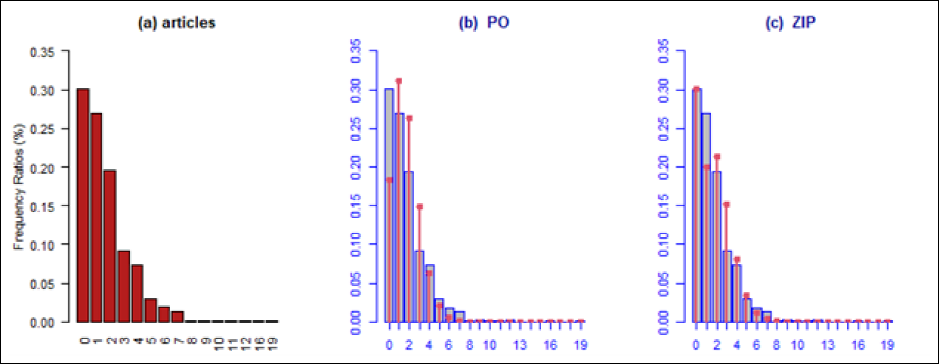
Before model fitting, variable selection was conducted. The predictor x1 was excluded from nonparametric consideration due to its categorical predictor. Furthermore, based on a comparison of the coefficients of determination for the continuous variables x2 and t, variable t exhibited a lower coefficient of determination, indicating a weaker linear relationship with the response variable. Consequently, variable t was deemed suitable for nonparametric treatment in the semiparametric models. Figure 3 shows the plots produced with two distributions for the dependent variables (count) in the ‘bioChemists’ data, where the proportion of zeros in the dependent variable was equal to 30 per cent. Figure 3 utilizes vertical lines topped with circles to represent the distribution fits.
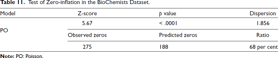
Test of Zero-inflation in the BioChemists Dataset.
LR Tests for Fitted Regression Models.
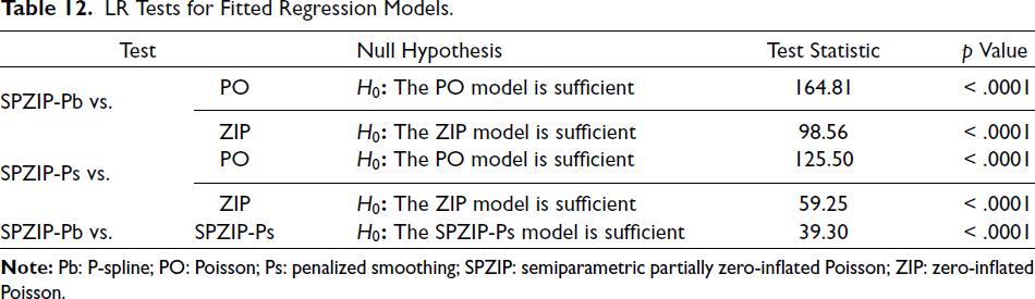
Figure 3 highlights how important it is to use the ZIP distribution when the data suffer from the problem of excess zeros. When comparing the ZIP distribution and the PO distribution in representing the percentage of zeros in the data, it becomes clear that the PO distribution captured only 20 per cent as zeros, while the ZIP distribution captured 30 per cent as zeros. This emphasizes that the PO distribution is unsuitable for data with excess zeros and can lead to inaccurate representations. Furthermore, we applied the Z-score test to check for overdispersion where H0: equidispersion versus H1: true dispersion is greater than one. The test results in Table 11 also show that the Z-score statistic is 5.67 with a significant p value < .001, thus we can reject H0, which means that the true dispersion is greater than one, meaning that the dataset has an overdispersion problem. The estimated dispersion value of 1.856 further supports this conclusion.
In addition, from Table 11, the amount of observed zeros is larger than the amount of predicted zeros, this means the model is under-fitting zeros, which indicates a zero inflation in the data. Table 12 presents likelihood ratio (LR) test results comparing the SPZIP regression model, estimated using both Pb and Ps estimators, to the PO and ZIP regression models. The null hypothesis (H0) for each comparison posits that the simpler regression models (PO or ZIP) adequately explain the data, whereas the alternative hypothesis (H1) asserts that the SPZIP regression model provides a significantly better fit. The results of the LR tests yield consistently high chi-squared test statistics and low p values, strongly supporting the superiority of the SPZIP regression model in capturing the underlying data patterns relative to both the PO and ZIP models. Furthermore, the analysis indicates that the SPZIP regression model estimated using the Pb estimator provides a significantly better fit than the SPZIP model estimated with the Ps estimator, with a highly significant LR test statistic (p < .0001). These findings suggest that the SPZIP regression model utilizing the Pb estimator captures the underlying data patterns with greater accuracy than all models considered.
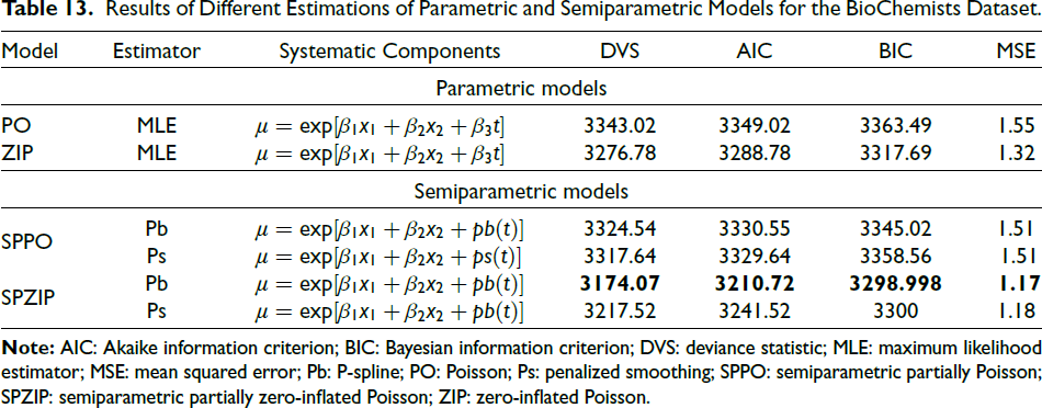
As shown in Table 13, four statistical regression models were estimated, including two parametric models (PO and ZIP) and two semiparametric models (SPPO and SPZIP). The semiparametric models were employed to capture nonlinear relationships in the data. The models were compared based on three selection criteria, that is, AIC, DVS and MSE. The SPZIP regression model with Pb estimator achieved the lowest values for all three criteria, indicating it is the best-fitting model.
Results of Different Estimations of Parametric and Semiparametric Models for the BioChemists Dataset.
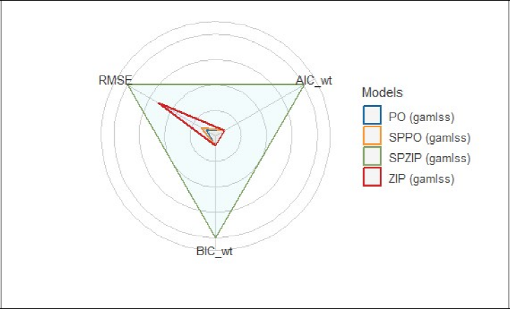
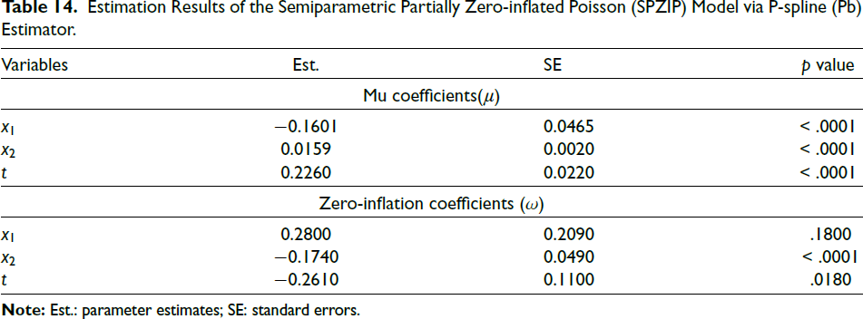
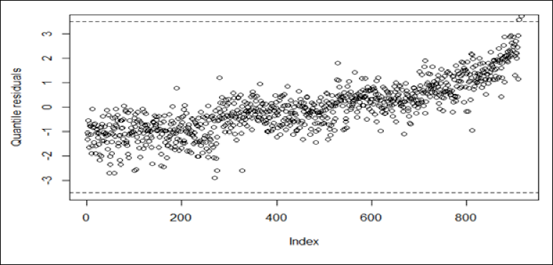
Accordingly, Table 14 presents the parameter estimates (Est.), standard errors (SEs), and p values for the SPZIP regression model via Pb estimator. At the 5 per cent significance level, all explanatory variables are statistically significant. Figure 4 presents a radar plot comparing the performance of four statistical regression models (PO, ZIP, SPPO and SPZIP) via Pb estimator across three evaluation metrics: RMSE, AIC weight (AIC_wt) and BIC weight (BIC_wt). Lower values generally indicate better model performance. The SPZIP regression model via Pb estimator appears to be the most balanced performer, with relatively low values across all three metrics. Overall, the SPZIP regression model seems to offer a good compromise between predictive accuracy and model complexity, making it a strong contender for further analysis. Additionally, Figure 5 presents a plot of the quantile residuals against the index of observations for the fitted SPZIP regression model. The quantile residuals generally fall within the expected range of [–3.5, 3.5], with only two outliers. Furthermore, the residuals exhibit no discernible patterns, suggesting that the model adequately captures the underlying data structure.
Estimation Results of the Semiparametric Partially Zero-inflated Poisson (SPZIP) Model via P-spline (Pb) Estimator.
Quantile Residuals for the Fitted Semiparametric Partially Zero-inflated Poisson (SPZIP) Regression Model.
Conclusions
This article has introduced two extensions of count data models (SPPO and SPZIP). These models build upon the PO and ZIP regression models, respectively. The key innovation lies in incorporating a nonparametric component estimated via Pb and Ps estimators. This nonparametric component allows for more flexible modelling of the relationship between covariates and the response variable. A Monte Carlo simulation study, under different scenarios, and a real data application were conducted to evaluate the robustness of introduced estimators. We relied on five criteria (AIC, BIC, DVC, MAE and RMSE) to identify the best-performing estimator. Based on the results of the simulation study and a real-data application, the estimators consistently achieved lower values across all metrics, suggesting their superiority. The ZIP.pb estimator emerges as particularly effective for analysing complex count data. Notably, the SPZIP model utilizing the Pb estimator proved particularly effective for analysing complex count data.
Insert two statements before Reference section:
Footnotes
Declaration of Conflicting Interests
The authors declared no potential conflicts of interest with respect to the research, authorship and/or publication of this article.
Funding
The authors received no financial support for the research, authorship and/or publication of this article.