
Abstract
Item response theory (IRT) is not widely used in counseling psychology research, despite its considerable advantages for instrument development. Focus groups help create a broad and representative item pool that is more likely to tap the full range of the latent dimension, thereby capitalizing on IRT strengths. We provide suggestions for using these tools, with an empirical example, the Everyday Multicultural Competencies/Revised Scale of Ethnocultural Empathy (EMC/RSEE). Rasch IRT methods were used to (a) analyze response format performance and collapse poorly performing categories, (b) evaluate differential item functioning sex bias, and (c) select items to maximize subscale sensitivity and bandwidth. Traditional classical test theory (CTT) subscales composed of items with the highest factor loadings were compared with subscales based on IRT criteria. Compared with CTT subscales, IRT subscales used in the EMC/RSEE demonstrated generally higher correlations with other variables of interest, and superior sensitivity to change over time and to group differences.
Perhaps no other single scholarly activity advances research more rapidly than developing a useful instrument, especially when the effort represents the first operationalization of a theoretical construct. For example, the general concept of the working alliance had its roots in the psychotherapy literature extending back decades before Greenson’s (1967) book, which specifically described the term. However, in the 5 years following its publication (i.e., 1968-1972), only four peer-reviewed articles were indexed under the PsycINFO thesaurus term therapeutic alliance. In 1976, Bordin’s seminal paper prompted further interest, yet in the 10-year period from 1977-1986, only 31 peer-reviewed articles appeared on the therapeutic alliance. A perceptible change began when the Working Alliance Inventory (WAI) was introduced in a book chapter (Horvath & Greenberg, 1986), and later in a journal article (Horvath & Greenberg, 1989), thereby joining several other measures of the psychotherapy relationship. From 1986-1990, only 57 peer-reviewed articles had been published on the therapeutic alliance, but in the next 5 years (1991-1995) after the WAI became widely available, the number burgeoned to 143.
Thus, developing the initial measure of an interesting construct can stimulate a rapid expansion of research, which is widely recognized as a great benefit for the field. However, less widely recognized is that once a consensus develops in the research community around relatively exclusive use of a specific measure, the instrument often influences conceptualization of the construct itself in ways that may be detrimental. For example, when beginning doctoral students are introduced to the concept of the working alliance at our institution, their readings include a description of Bordin’s (1976) tripartite bonds/goals/tasks model, together with a copy of the WAI. The strong implication is that the working alliance is what the WAI measures—no more and no less. As a result of practices like these, few new researchers, and fewer still contemporary practicum students, realize that “Patient Commitment” to therapy was assessed formerly by one of the five factors of the California Psychotherapy Alliance Scales (CALPAS; Gaston, Marmar, Thompson, & Gallagher, 1988). This facet of the alliance construct seems to have passed largely out of contemporary awareness, as the WAI supplanted the CALPAS.
Fortunately, client commitment to the change process reemerged as a key construct in the stages of change theoretical model (Prochaska & Norcross, 2001). Perhaps truly useful constructs do not become permanently “extinct,” even when the research community stops using the initial assessment measure. However, the established dominance of the WAI in contemporary psychotherapy research should prompt questions such as the following: Is patient commitment an inconsequential facet of the therapeutic alliance construct?, Is it appropriately considered to be a component of the construct at all?, and If so, is it fully subsumed within the 36 items of the WAI? Answering these questions is beyond the scope of the present article, but posing them serves to underscore the great responsibility in instrument development research to assure the content validity of the resulting scale.
Content validity is established by showing that the test items are a sample of a universe in which the investigator is interested. Content validity is ordinarily to be established deductively, by defining a universe of items and sampling systematically within this universe to establish the test. (Cronbach & Meehl, 1955, p. 282)
Thus, Cronbach and Meehl’s definition sets forth two essential tasks to establish content validity in every instrument development project: (a) defining the universe of items and (b) systematically sampling this universe. Unlike criterion-related validity, there are no straightforward statistical coefficients to assess how adequately these content validity tasks have been performed. Instead, our evaluation must be based on the quality of the research procedures described by instrument developers. The first thesis of this article is that focus groups are a valuable and underutilized aid for ensuring quality of the first of Cronbach and Meehl’s content validity tasks, namely defining the universe of items. This is especially true of the initial effort to develop the measure of a construct. Our second thesis is that the quantitative methods of item response theory (IRT) can be very helpful in the remaining content validity task, that of selecting a representative sample of items from this universe.
Given the importance of scale development as a research activity, and its daunting problems in terms of both research design and quantitative methods, it is not surprising that Worthington and Whittaker’s (2006) article providing guidelines in this complex area has become one of the most frequently cited recent works in the counseling psychology literature. However, Worthington and Whittaker (2006) intended only to provide recommendations for best practices in application of exploratory factor analysis (EFA) and confirmatory factor analysis (CFA). Their suggestions are made primarily from the standpoint of classical test theory (CTT). Therefore, the purpose of the current article is to supplement their work with (a) suggestions for using focus groups in the initial stage to generate a broadly inclusive initial item pool and (b) suggestions about using IRT to benefit the later stages of scale development in which the final set of items are selected. To illustrate these advantages, we will provide examples of focus group procedures and IRT analyses used to develop an instrument designed to assess outcomes of undergraduate multicultural programming by Mallinckrodt et al. (2014), the Everyday Multicultural Competencies/Revised Scale of Ethnocultural Empathy (EMC/RSEE).
Using Focus Groups to Generate an Item Pool
In a review of the most frequent “fatal flaws” of manuscripts that were rejected from the Journal of Counseling Psychology without an opportunity for the authors to revise, Hoyt and Mallinckrodt (2012) emphasized the importance in instrument development research of establishing that the initial item pool “contained a sufficient number of items to tap each critical aspect of the overarching construct . . . [and was not] constricted by the researchers’ potentially limited perspective” (p. 75). They went on to advocate use of focus groups to improve content validity, especially when the researchers themselves have had little direct life experience of the construct. Therefore, as a general strategy for instrument development, we recommend a mixed methods research approach (Hanson, Creswell, Plano Clark, Petska, & Creswell, 2005), in which an initial qualitative phase employing focus groups is used to generate a comprehensive item pool that is then refined through a subsequent series of quantitative analyses, including IRT. Mixed methods research offers advantages for understanding cultural influences and context from multiple perspectives (Klassen, Creswell, Plano Clark, Clegg Smith, & Meissner, 2012). Furthermore, the sequential mixed methods design we advocate for instrument development closely integrates qualitative and quantitative components, allowing researchers to benefit from the advantages of both approaches (Castro, Kellison, Boyd, & Kopak, 2010).
Using a sequential mixed methods design in the development of the EMC/RSEE, we first solicited focus groups to aid in developing a comprehensive pool of items. Specifically, we convened three focus groups: (a) one with campus administrators, (b) one with graduate instructors of an introductory psychology course, and (c) one with residence hall peer advisors. Members of the third group not only delivered diversity programming but were also recipients of programming through their in-service training. Group members who are representatives of the population of interest, such as these, offer the additional advantage of generating items in the natural language of the group. In addition, unlike a series of individual interviews, focus groups offer advantages that stem from the group dynamics of members’ interactions with each other, which can serve to enhance the overall richness of the data and generate a shared understanding of the construct (Flick, 1998).
Each group worked independently and was presented with the following operational definition:
Imagine a bright, ambitious undergraduate senior graduating from a large public university. Considering the range of multicultural environments, both in the U.S. and abroad, that this student is likely to experience in a productive career, please discuss the following three questions: (a) What are the attitudes, personal awareness, and ways of thinking that this student should possess to function effectively? (b) What are the skills that this student must acquire to function effectively? (c) What bases of knowledge must this student have to function effectively? (Mallinckrodt et al., 2014, p. 135)
Developing an operational definition in nontechnical language for the focus groups can push a research team to think more carefully about the boundaries of the construct. Publishing the exact definition used to generate items gives readers a better sense of the instrument and its limitations. For example, because the race/ethnicity of the “bright, ambitious undergraduate senior” was not explicitly specified, and the instrument was developed on a predominantly White campus, the EMC/RSEE cannot claim to tap the everyday multicultural competencies of racial and ethnic minority students.
Most focus group members will lack the technical expertise to generate items that can be used directly, and items suggested by members will need to be closely edited for flaws such as double barreled wording. However, members of a carefully selected focus group will possess a different kind of expertise—one that researchers themselves often lack, namely, direct life experience with the construct of interest. Thus, focus group members are often in a particularly advantageous position to compensate for researchers’ blind spots, by suggesting components of the construct and domains of content that may not have occurred to the researchers themselves. Compared with a series of individual interviews, focus groups offer the advantages of time efficiency, and more importantly, members stimulate one another and elaborate on each others’ comments. Thus, the group as a whole offers a potentially much richer contribution than the sum of its individual members. We will not reiterate the excellent general guidelines available for facilitating research focus groups (e.g., Carey & Asbury, 2012; Krueger & Casey, 2009). For the specialized task of identifying the “universe of items,” to use Cronbach and Meehl’s (1955) term, after providing a working definition of the construct, we recommend a series of question prompts that move from a broader to a narrower focus. As an online supplement, we have provided a series of prompts designed especially to stimulate divergent thinking and the broadest possible exploration of the construct universe (http://tcp.sagepub.com/supplemental). However, note that these prompts are tailored for highly educated focus group members such as those we solicited in developing the EMC/RSEE.
In facilitating these focus groups, it is important not to close off the process by prematurely moving to the next stage. We suggest the following sequence: (a) begin by identifying broad dimensions and themes abstracted from anecdotes of personal experience; (b) probe the construct boundaries and ensure that all relevant dimensions have been identified; (c) probe for divergent thinking and alternative dimensions and themes; (d) systematically return to each dimension, asking members to generate positive and negative examples; (e) for each dimension, consider prompting group members to generate items, ideally to include some at extremely high and low levels of this theme; and finally (f) consider holding two meetings approximately 1 week apart and, at the second meeting, share initial results for all groups, having each respond and repeat an expedited version of Steps a to e. Generating items (Step “e”) may not be appropriate for groups whose members lack extensive experience with self-report survey items. In these circumstances, researchers will emphasize Step “d,” the stage of offering examples of the construct components instead of proposing items. Focus group members with limited education and low English reading levels can nevertheless be ideal informants if they are representative of the population researchers intend to survey. The vocabulary used by these group members to discuss their life experiences will help researchers guard against constructing a measure whose reading level is inappropriate for the samples they intend to use.
To generate an initial item pool, the research team should transcribe and review audio recordings of each focus group. Although focus group participants may be asked to suggest items directly, most of the research team’s work will involve converting the anecdotes and exemplars offered by group members into items. Researchers must craft final wording to present concise and unambiguous stimuli. (For helpful suggestions, see DeVellis, 2003.) Outside consultants can be very helpful to review items for content and clarity (Worthington & Whittaker, 2006). Thus, a second type of focus group may be helpful at this stage, one that reviews and edits a preexisting item pool instead of aiding in the generation of the items.
Researchers must also give careful attention to selecting an appropriate response format or formats for the item pool. Likert-type, semantic differential, and frequency-based formats (e.g., never, sometimes, often . . . ) are among the most frequently used in counseling psychology research. A discussion of the unique advantages and disadvantages of each format is beyond the scope of this article. However, an essential ingredient of any format is that the steps between all neighboring pairs of responses should represent equal measurement intervals. Thus, in a frequency format if “rarely” and “occasionally” are neighboring pairs, this interval must be equivalent to the difference typical respondents assign to other neighboring pairs such as “sometimes” and “always.” Recent research suggests that the assumption of equidistant measurement intervals may be questionable for many frequency-based response formats (Bocklisch, Bocklisch, & Krems, 2012). The number of response categories to present is also a critical methodological choice. In general, additional categories increase reliability, but only up to the point that respondents can make meaningful distinctions among them (Bond & Fox, 2007). Instrument developers typically generate both positively and negatively worded items to prevent response-set bias (Paulhus, 1991). However, recent IRT research suggests that negatively worded items may not assess the same latent construct as positively worded items, and can introduce an independent confounding dimension, as well as inflate estimates of scale reliability (W. Wang, Chen, & Jin, 2015).
Sample Size Considerations
After careful editing, revision, and removal of obviously redundant and otherwise undesirable items, a large item pool may still remain. The richness and variety of items created through the focus group process presents a dilemma. In choosing how many items to retain for presentation to survey participants, researchers must balance (a) consideration of coverage and range in the number of items retained for presentation, versus (b) having a sufficient sample size to support EFA with a separate holdout sample for CFA. Worthington and Whittaker (2006) cited experts such as Gorsuch (1983) who recommend minimum ratios of participants to items of 5:1 to 10:1 for EFA, but they emphasize that item-factor loadings and commonality values also govern the adequacy of sample size. For CFA, Worthington and Whittaker (2006) suggested that a sample size of 300 is “generally sufficient in most cases” (p. 817). A larger sample is required as the number of factors and complexity of the model increases. Based on these guidelines, we suggest the following formula to estimate the minimum number of subjects N that are required for an item pool of size P:
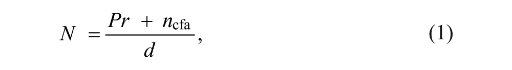
where r = the minimum number of participants per item needed to support EFA; ncfa = size of the subsample held out for CFA; and d = the proportion of the sample expected to provide useable responses.
With regard to the value of d, some empirical studies report rates of inattentive responding on self-report inventories ranging from 3%-9% (Maniaci & Rogge, 2014) to 10%-12% (Meade & Craig, 2012). Findings suggest that failure to correct for this problem can obscure otherwise significant results in both regression and experimental studies (Maniaci & Rogge, 2014), as well as factor analyses (Meade & Craig, 2012). Our own experience over 20 years at three universities suggests that 10% to 25% of undergraduates who receive extra credit for participation in survey research routinely fail to correctly answer validity-check items such as “Please code a five for this item” or “Please leave this item blank.” Maniaci and Rogge (2014) referred to items like these as directed questions, and suggested that they should be embedded in the items of approximately every other page of a paper and pencil survey. Thus, we strongly suggest that researchers include such items in their scale development survey. We use a ratio of about one validity check per 30 to 40 items presented. It is probably best to exclude all data from surveys with answers to these items that suggest inattentive or random responding. Mallinckrodt et al. (2014) reported that 13% of responses were excluded for this reason in developing the EMC/RSEE.
The value of d, the invalid survey response “discount,” should also account for cases with large amounts of missing data. Mallinckrodt et al. (2014) deleted cases with more than 10% of the items missing and estimated missing values for the remaining cases with less than 10% missing data using an expectation maximization procedure. It appears that a consensus has not yet developed about how much missing data may be too much to support estimation methods in factor analysis (Harrington, 2008). A detailed treatment of missing data is beyond the scope of this article, but we note these three points: (a) the pattern of missing data is a more important consideration than the proportion missing, (b) mean substitution is not appropriate for handling missing data, and (c) detailed guides for missing data techniques are available (e.g., Harrington, 2008; Schlomer, Bauman, & Card, 2010).
For the EMC/RSEE, after deleting cases with invalid responses, an additional 3.3% of cases were discarded due to more than 10% missing data, resulting in a combined loss of 16.3% of the sample. Thus, we recommend adopting a value of 0.8 for d. Following Worthington and Whittaker’s (2006) guidelines, for ncfa we suggest a value of 300 or 33% of N, whichever is larger. Adopting a value of 5 for the critical ratio r, and solving for N in Equation 1:


Thus, approximately 6.25 subjects for each item presented, plus 375 additional holdout subjects for CFA, represent a minimum sample size. For example, if researchers decide to retain 100 items in the initial pool, we recommend a minimum sample of 1,000 subjects. Adopting a more conservative critical ratio r of 8:1 would require about 10 times the number of subjects as items, plus 375 more subjects for CFA.
We suspect that practical considerations about the available sample size often drive researchers’ choices about the size of the item pool they present for analysis. We believe this reverses the appropriate priority, given the importance of ensuring content validity. Instead of shrinking the item pool to meet the constraints of the sample size, it is critical to make efforts to gather a sufficiently large sample to support analysis of an adequate item pool. After removing obviously redundant and poorly worded items, the remainder of the item pool should be presented. Researchers cannot know in advance how many dimensions will emerge from EFA. As we will show in the discussion of subscale bandwidth and test information in the next section on IRT, it is especially important to present items that represent endpoints of the hypothesized dimensions, as well as representative points all along the continuum.
The list of suggestions in the appendix begins with a summary of procedures for using focus groups to generate an initial item pool. We have presented considerable detail because we believe these points have not received sufficient attention in the counseling psychology literature. As Hoyt and Mallinckrodt (2012) emphasized, no manuscript revisions can salvage a scale development study based on an inadequate initial item pool (e.g., one that does not adequately sample each region of Cronbach & Meehl’s, 1955, “universe of items” for the target construct). Serious questions about content validity constitute a fatal flaw in such studies. After a sufficiently broad and representative item pool has been analyzed with the EFA procedures recommended by Worthington and Whittaker (2006) to identify factors and assign items to these dimensions, the techniques of IRT described in the next section can be used to inform the final selection of items.
Overview of IRT
Excellent, in-depth articles describing recent developments in IRT theory and methods are available (e.g., Cai, Yang, & Hansen, 2011; Ligtvoet, Van der Ark, Bergsma, & Sijtsma, 2011). However, as Wampold (1998) pointed out with regard to IRT, journals that specialize in research innovations, such as Psychological Methods or Psychometrika, are not widely read by counseling psychologists. Wampold urged that innovations in research methods should be tailored specifically to a counseling psychology audience, with appropriate mathematical rigor and relevant examples so that “proximity of explanation leads to adoption” (p. 46). We focus on the considerable advantages of using IRT to (a) produce scales that maximize sensitivity to detect change or group differences, (b) reduce problems with ceiling or floor effects by increasing bandwidth of a scale, and (c) reduce sex bias and other forms of differential item functioning (DIF). We begin by contrasting the theoretical assumptions of IRT with CTT. Next, we briefly describe various IRT models with emphasis on one variant, the Rasch model. Finally, we provide a step-by-step guide for using the Rasch model.
IRT is concerned with the process of scaling in measurement, that is, how a set of observed manifestations of a latent variable can be quantified to infer varying amounts of the construct and the relative position of individuals along the implied continuum (de Ayala, 2009). IRT is often contrasted with CTT, which is concerned with an individual’s summed score on a set of items. This sum provides an estimate of this person’s true score, operationally defined as the hypothetical mean of a set of summed scores taken over an infinite number of test administrations. Of course, any given actual test score is unlikely to match the true score (if the true score could be known). Thus, in CTT, an observed score is composed of two elements, the true score and a random error component. Harvey and Hammer (1999) summarized several important differences between CTT and IRT. CTT focuses more on properties of an entire scale, whereas IRT is concerned with the performance of individual items as they contribute to overall scale performance. Second, CTT assumes that a scale is equally accurate throughout the full range of possible scores, whereas IRT methods can be used to empirically examine whether a scale is more sensitive at discriminating, for example, among low-scoring individuals or among those scoring at the high end of the latent continuum.
Thurstone (1928, cited in de Ayala, 2009) defined invariance as the desirable property of a scale in which its functional usefulness as a measure is not influenced by properties of the measurement target, that is, the length of a ruler does not change as a result of the height of the person being measured. However, in CTT, the psychometric properties of a scale cannot be estimated apart from the performance of a specific sample. Thus, scale invariance cannot be achieved through CTT methods alone. The principles of CTT are invoked when students are admonished not to describe a scale as intrinsically valid or reliable because these psychometric properties are characteristics of scale scores estimated from a specific sample (de Ayala, 2009). However, the more robust assumptions of IRT do permit considerations of scale invariance. IRT methods can be used to estimate an individual’s ability, entirely apart from the specific set of items used in the assessment, and to estimate the difficulty of a specific item, completely independent of any specific sample of test-takers (Fox & Jones, 1998). (As described in the next section, the use of the terms ability and difficulty reflect the academic roots of the Rasch model of IRT.)
A wide range of IRT methods have evolved, including nonparametric and parametric approaches. The IRT parametric methods are distinguished by the number of estimated parameters. The Rasch approach is a variation of the general one-parameter logistic (1-pl) IRT model and has the advantage of determining a single score location along the hypothesized latent measurement construct (Doucette & Wolf, 2009). In addition to the basic item-difficulty/person-ability dimension in Rasch and 1-pl approaches, 2-pl methods add an item discrimination parameter that can be very useful when researchers are interested in comparing the relative power of an item, compared with other items, to discriminate individuals at specific points along the latent dimension (de Ayala, 2009). The 3-pl approach adds the capacity to assess respondent guessing, whereas the 4-pl model adds a parameter to assess careless responding (Linacre, 2004) that also may have some useful application in the study of psychopathology (Reise & Waller, 2003).
For research that emphasizes subjects’ performance, and in which guessing is an important parameter, the 3-pl model is preferred. The 2-pl model is preferred when theory or previous research suggests that items of the same difficulty vary in their power to discriminate among subjects on the hypothesized continuum, or when researchers wish to investigate the level of this discriminability. The 1-pl and Rasch models assume that discrimination coefficients are equal for all items. Critics point to this assumption as one of the most serious limitations of the Rasch model, and observe that its stringent data requirements for unidimensionality, equal discrimination by all items, and response to an item independent of responses to any other item are not likely to be met in real world research settings. For a review of this critique, see Panayides, Robinson, and Tymms (2010). In contrast, proponents of the Rasch model (cf. Andrich, 2002) argue that it describes ideal properties of data, and of course no actual data set will perfectly match these properties. Research suggests that Rasch analyses are fairly robust to violations of the model’s assumptions of dimensionality and equal discrimination parameters (Forsyth, Saisangjan, & Gilmer, 1981; van de Vijver, 1986).
The Rasch model has the desirable feature of specific objectivity, which allows the assumption of an invariant ranking of item difficulty independent of the abilities of individual test-takers (as well as an invariant ranking of person ability independent of the difficulty of specific items). Specific objectivity is a necessary assumption for creating equivalent parallel forms of an instrument. Furthermore, the assumption of specific objectivity leads directly to the desirable property of simple additivity in Rasch models, namely,
if one person is more likely to get an item with a specific level of difficulty correct than is another person, then this holds true for items with any level of difficulty . . . But with the addition of the discrimination parameter . . . the probability of endorsing an item as a function of ability will vary as a function of the item difficulty. (Revelle, 2013, p. 252)
In other words, adding a second parameter that allows items to differ in their discriminability eliminates the desirable feature of simple additivity provided by Rasch models, whereas preserving additivity makes possible direct comparison of individuals and test items across different testing circumstances.
Among IRT experts, debate about the appropriateness of the Rasch model evokes considerable energy, and has been described as “the Rasch Wars” (McNamara & Knoch, 2012). Rasch model versus other approaches embody quite different fundamental philosophies of measurement (de Ayala, 2009). Thus, the Rasch model shares all the fundamental differences in assumptions described previously that separate all IRT approaches from instrument development via CTT. Further, the Rasch model stands apart from the family of all other IRT approaches. Whereas other IRT approaches seek to find the best model to fit the available data, the Rasch approach starts with an idealized measurement model and estimates how well the available data fit this model (Andrich, 2002). Given the relative strengths and weaknesses of the models, Panayides et al. (2010) argued that if a researcher’s purpose is primarily to model existing test data, then multiple parameter models are preferred because they make less stringent assumptions than the Rasch model. However, the Rasch model is preferred for test construction because the 2-pl and 3-pl models
typically pose more problems during parameter estimation, fit assessment and interpretation of results. Whenever possible it is thus recommended to find a set of items that satisfy the Rasch model rather than find an IRT model that fits an existing item set. (Fischer & Molenaar, 1995, p. 5, as cited in Panayides et al., 2010)
Thissen and Wainer (1982), based on their examination of the relationship between sample size and asymptotic standard error, agreed that researchers should examine simpler models first, starting with the 1-pl.
If it fits rejoice and stop . . . [alternatively] . . . If only a few items (a small proportion) cause the lack of fit, and they do not form a coherent grouping in terms of subject matter of the test, consider omitting them from the test and continuing. (Thissen & Wainer, 1982, p. 410)
When the reduced model still does not fit the data, and no further item omissions can be justified, Thissen and Wainer suggested examining the 2-pl model next, followed only if necessary by the 3-pl approach. Thus, although the assumption of equal discrimination coefficients cannot be met in any set of real world items, the relevant question is whether differences in discrimination can be safely ignored.
We recommend the Rasch model for counseling psychology instrument development when (a) circumstances do not require estimating the effects of guessing and (b) the advantages of specific objectivity and sample independence outweigh the disadvantages of assuming all items have equal discrimination coefficients. Another advantage of the Rasch model is that its simplicity and parsimony permit sophisticated analyses of whether the instrument’s response scale functions as intended. Note that the Rasch and 1-pl models are sometimes described as being quite similar, but they are not synonymous. Both models assume a constant level of the discrimination parameter, α, across all items. However, the philosophical assumptions of the Rasch model impose the additional constraint that α = 1.0 always, whereas the 1-pl model allows α to assume different values for a set of items from one instrument to another (de Ayala, 2009).
Rasch Model Approach to Scale Development
Key assumptions of unidimensional Rasch IRT models are that subscale items serve as observed indicators of a single underlying latent construct (Bond & Fox, 2007), and that this underlying construct has properties of invariance that can be used to locate persons with respect to their ability, and items with respect to their difficulty. These terms reflect the roots of the Rasch model in developing measures of academic performance, using items that can be scored dichotomously as either correct or incorrect. Although not accurate in the strictest sense, the terms ability and difficulty can also be applied as a useful heuristic in describing assessment of traits or attitudes. Therefore, as we consider progressively higher locations along the latent dimension of an underlying trait or attitude, persons of increasing ability have increasing likelihood of endorsing more difficult items (i.e., those that express the trait or attitude in stronger or more extreme terms). In a parallel fashion, the most difficult items are those whose probability of being endorsed is highest among persons with the highest ability (i.e., persons who possess this trait or attitude most strongly). By convention, the Greek lowercase theta, θ indicates person location, and delta, δ, is most often used to indicate item location on the same latent dimension (although b is also sometimes used, as in Figure 1). In IRT analyses of academic performance scales, an item is scored as correct for a response choice that indicates higher proficiency; whereas in analyses of trait or attitude scales, the correct scoring of an item is in the direction of stronger endorsement of the attitude or presence of the trait.
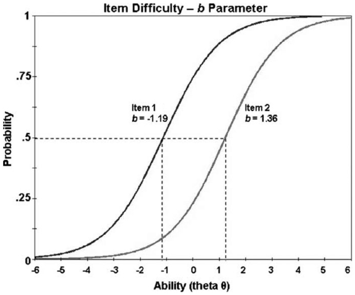
Comparison of two item characteristic curves.
These concepts are illustrated in Figure 1, adapted from Doucette and Wolf (2009). For simplicity, the two items portrayed are dichotomous and graphed with the probability of a correct answer depicted on the y-axis. The latent construct is graphed on the x-axis, with increasing ability of individuals with respect to this construct increasing from left to right. The x-axis scale is in logit units 1 , which can be used as a standardized index for both persons and items. The difficulty, b, of a particular item is given by examining the location on the x-axis corresponding to the ability level of individuals who have a .50 probability of answering that particular item correctly. Figure 1 shows that Item 1 is relatively easier than Item 2, as indicated by the vertical line descending from the .50 point of inflection in the probability curve of Item 1 (b = −1.19), which falls to the left of the corresponding vertical line for Item 2 (b = +1.36). We can also see, based on where the dashed line at an ability of −1.19 cuts across the Item 2 curve, that persons at this ability, who have a .50 probably of answering Item 1 correctly, have only about a .10 probability of answering Item 2 correctly. IRT methods can be used to plot item characteristic curves like these (sometimes also called item response functions or item response curves) for the difficulty of each item in a measure. The difficulty of a given item, therefore, is defined as the ability level of individuals who have a 50% probability of answering that item correctly, and the ability of a particular individual is determined by her or his probability of a correct response to items of varying difficulty. Note that Figure 1 also shows an important feature of the Rasch model, namely, that the slope of a curve (representing the discrimination parameter, α) is identical for all items. A shift along the x-axis represents only a change in difficulty.
Thus, in the example that follows, we will refer to items assessing multicultural constructs in terms of difficulty and the level of multicultural knowledge, skills, or attitudes of a person as that individual’s ability. The great advantage of the Rasch model is that both can be plotted using the same metric (i.e., logit units) on the same scale to represent the latent construct. Thus, location refers to both item difficulty and person ability. In Rasch analysis, the difficulty of an item is estimated independent of the ability of any particular sample of test-takers, and the ability of an individual is estimated independent of any particular set of assessment items. In the software that calculates these coefficients, provisional estimates for ability in the sample of persons are used to estimate item difficulties, which are then used to refine estimates of persons’ ability, and so on iteratively until the process of calibration converges on stable estimates. As illustrated in the example provided in the next section, item difficulty estimates can be very useful when making the final selection of items to retain for a scale that a researcher wishes to shorten.
Although Rasch methods were originally developed with items that have a single correct response (e.g., true/false or multiple choice), Rasch analyses are well adapted for use with polytomous response formats, that is, those that have multiple response points and no single correct answer, for example, frequency formats (e.g., always, sometimes, never) or Likert-type multiple responses indicating varying levels of agreement (e.g., strongly agree, agree, disagree, strongly disagree). Two forms of Rasch polytomous models are the partial credit approach, appropriate when the number of responses varies across items and measurement distance between response points is assumed to vary, and the rating scale model, which is appropriate when the same rating format is used for every item (Fox & Jones, 1998). Because the EMC/RSEE adopted a 6-point Likert-type scale for every item (1 = strongly disagree, 2 = moderately disagree, 3 = slightly disagree, 4 = slightly agree, 5 = moderately agree, 6 = strongly agree), the rating scale Rasch polytomous model was used in the example that follows. Thus, instead of a single difficulty coefficient as would be observed for a dichotomous item, Likert-type items yield k − 1 difficulty thresholds, each at a different location along the latent continuum.
Figure 2 provides an illustration for Item m65 from the initial EMC/RSEE item pool, and shows option response functions (ORF) for each of the six categories in terms of probability of endorsement as a function of difficulty. Figure 2 shows that individuals below a location (i.e., ability) of approximately −2.4 logits are most likely to answer strongly disagree. This probability approaches 1.0 for the lowest values of person ability. The second ORF from the left is a bell-shaped curve corresponding to the difficulty of answering moderately disagree for Item m65, the third ORF represents slightly disagree, and so forth. Thus, each of the six possible responses to Item m65 from strongly disagree through strongly agree traces an ORF of increasing difficulty. Persons must exhibit progressively more of the underlying latent construct measured by Item m65 to endorse ever more difficult response choices. The five dashed lines indicate thresholds between response categories. For example, the second threshold at a value of approximately −1.6 logits indicates that persons higher in ability than this value are more likely to answer slightly disagree (Category 3) than moderately disagree (Category 2). The Rasch approach estimates a single difficulty coefficient for a given item based on a combination of its category thresholds.
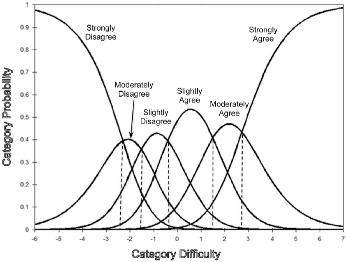
Option response functions and thresholds for a 6-point Likert-type item.
Illustrative Empirical Example
Participants
The data used in this example were drawn from a larger project that developed a multidimensional measure of “everyday multicultural competencies” to assess outcomes of diversity programming for college undergraduates (Mallinckrodt et al., 2014). Because the development of empathy is an important goal of many multicultural programs in higher education (e.g., intergroup dialogue; Khuri, 2004), we used the Scale of Ethnocultural Empathy (Y.-W. Wang et al., 2003) as a starting point. Details regarding the development of the item pool, as well as the EFA and CFA, and analyses used to estimate validity and reliability of scores, are described in Mallinckrodt et al. (2014). Surveys with more than 10% missing data were excluded, as well as those with answers to validity-check items (e.g., “Please code a seven for this item”) that indicated inattentive responding. Because we expected group differences, only data from students who reported their racial/ethnic identification as “White, European American” and also non-Hispanic were included in the instrument development phase of this project.
IRT methods require large samples. Wright (1997) suggested that samples of 500 are sufficient for Rasch calibration in most circumstances, but de Ayala (2009) cautioned that even larger samples may be needed for adequate factor analyses to check for unidimensionality or to check for appropriate functioning of response categories if responses are not equally distributed. (Note that unidimensionality is not an exclusive requirement of the Rasch approach). A total of 602 students in sections of introductory psychology provided usable data at Time 1, near the midpoint of Fall semester, and 676 provided useable surveys at Time 2, near the end of Fall semester. Of these, surveys from 326 students provided a repeated measures subset of Time 1 and Time 2 data. However, to preserve data independence, only one of the two surveys provided by these students was randomly selected and the other excluded. Thus, there were 952 independent cases available for instrument development, 276 Time 1 only students, 350 Time 2 only students, and 326 retest students randomly assigned to provide either 163 Time 1 or 163 Time 2 data sets.
EFA of the initial 115 item pool resulted in a six-factor solution that was interpretable and supported by a parallel analysis (Fabrigar, Wegener, MacCallum, & Strahan, 1999). IRT methods were used to develop all six subscales of the EMC/RSEE, essentially treating each as an independent measure. Mallinckrodt et al. (2014) reported that only one pair of subscales were correlated in absolute value >.50, and therefore, they did not recommend using a total scale score. Thus, technically speaking, the EMC/RSEE is a multiscale not a multidimensional instrument. Because Factor 2 provides an excellent illustration of how to use IRT methods, generally we will focus only on the subscale developed for Factor 2, Resentment and Cultural Dominance. However, we refer to other subscales when they provide a better example of a key concept. Factor 2 was one of two among the six EMC/RSEE factors that tapped negative attitudes or lack of perceived multicultural skills.
Screening Items for Unidimensionality
Following the recommendations of Worthington and Whittaker (2006), an item was assigned to Factor 2 if its loading was >.32, and it did not load within an absolute value of .15 on any other factor. This initial item selection procedure resulted in the retention of 81 items for the EMC/RSEE, with 21 assigned to Factor 2. An 81-item instrument would be too lengthy for practical purposes. The basic CTT approach to shortening a scale is to delete items with low factor loadings that contribute the least to subscale internal consistency (e.g., Worthington & Whittaker, 2006). These criteria follow from the basic assumptions of CTT, particularly the assumption that maximizing the covariance in a set of items will reduce the proportion of summed score variance due to error. Other experts (cf. Doucette & Wolf, 2009) advocate using IRT to generate additional empirical item selection criteria. We believe that IRT item difficulty and DIF should be included as additional criteria to reduce potential bias and create scales with optimal sensitivity to detect group differences or change over time.
Table 1 presents an example of how IRT criteria were incorporated into selection of the 21 items initially screened for Factor 2. The first column of coefficients displays item-factor loadings from the EFA. In using IRT criteria for a step-by-step reduction of Factor 2, we relied heavily on the suggestions of de Ayala (2009) and Bond and Fox (2007). All Rasch analyses were conducted using WINSTEPS 3.80 software (Linacre, 2013), applying a rating scale polytomous model to provide a point estimate of difficulty for each Likert-type item. (Note that WINSTEPS generates a syntax code file via a series of menu driven options. Thus, it is not necessary for users to write their own code.) Unidimensionality is a critical assumption in the Rasch IRT approach (Hambleton & Swaminathan, 2010). Specifically, to provide a useful basis for indexing the ability of persons and the difficulty of items, the latent construct must reflect only a single attribute. Unidimensional latent constructs permit the critical assumption of conditional or local independence; that is, estimates of a given item’s difficulty are completely independent from the responses given to any other item except for the trait they have in common (Fox & Jones, 1998). Under the assumption of conditional independence, an IRT model can account for all of the covariance between items entirely by describing the relationship of each item separately to the common underlying latent variable (Steinberg & Thissen, 1996). Speeded tests, for example, violate the assumption of conditional independence because responses are influenced by ability in the content area, together with a second dimension of general capacity for quick responding (de Ayala, 2009). In speeded tests, the correct response to an item later in the series is conditional on the time required to respond to all previous items.
Using IRT to Reduce Subscale Length
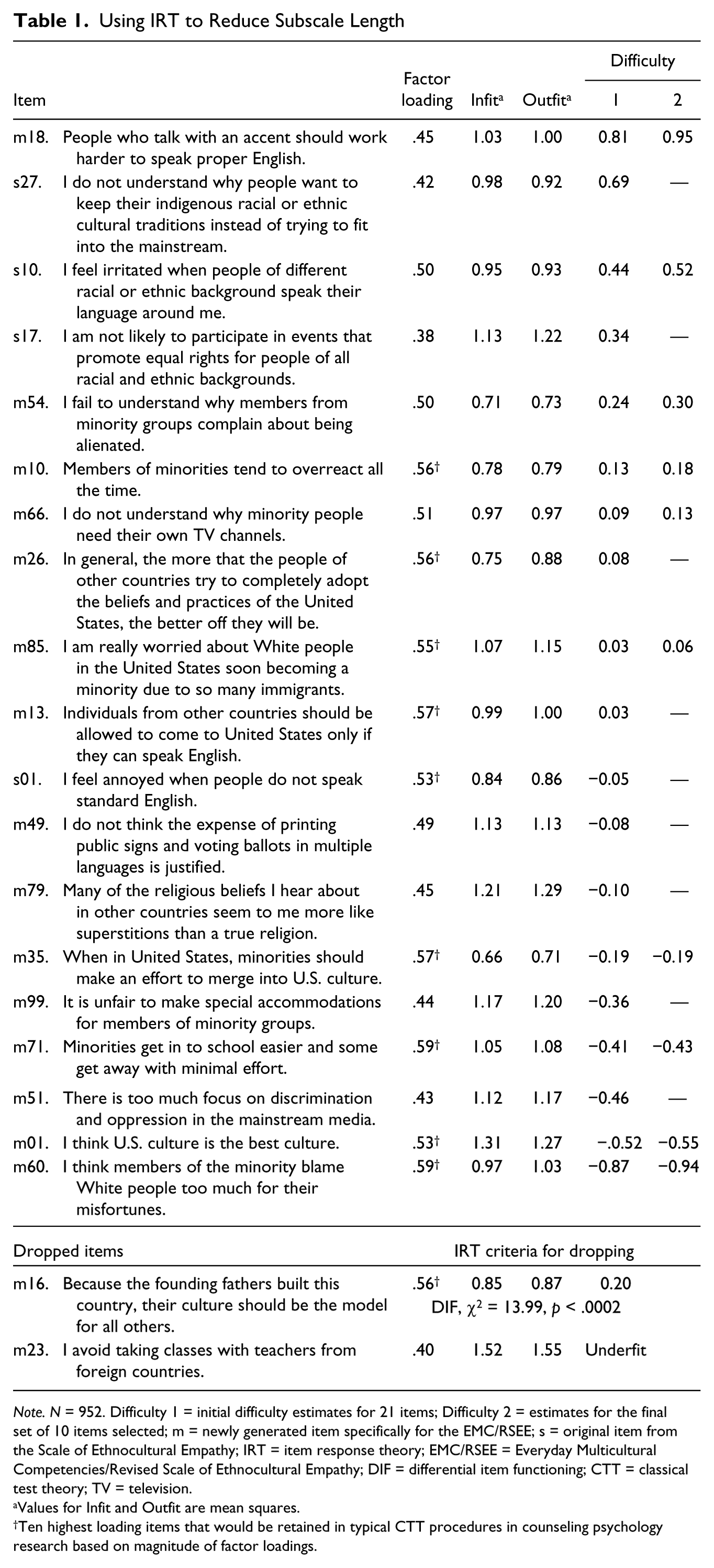
Note. N = 952. Difficulty 1 = initial difficulty estimates for 21 items; Difficulty 2 = estimates for the final set of 10 items selected; m = newly generated item specifically for the EMC/RSEE; s = original item from the Scale of Ethnocultural Empathy; IRT = item response theory; EMC/RSEE = Everyday Multicultural Competencies/Revised Scale of Ethnocultural Empathy; DIF = differential item functioning; CTT = classical test theory; TV = television.
Values for Infit and Outfit are mean squares.
Ten highest loading items that would be retained in typical CTT procedures in counseling psychology research based on magnitude of factor loadings.
Therefore, we began winnowing items by following the three-step sequence of progressively more stringent tests of unidimensionality suggested by Linacre (1998). First, we examined corrected item-subscale total correlations to be certain that all were positive and that the reverse keying required for negatively worded items was successful in creating a positive loading. (Note that negatively worded items must be recoded so that higher scores on every item indicate stronger endorsement of the latent construct.) This step also included examination of whether responses to the 6-point Likert-type scale for each item measured students as expected. Problematic items can exhibit disordered thresholds in which persons of higher ability are more likely to endorse the lower response of a pair (e.g., strongly disagree) than the neighboring higher point (e.g., moderately disagree). All Factor 2 items passed this screen, but two items assigned to Factor 1 did not. These two items were dropped because, for them, the Likert-type response scale did not differentiate properly between students of differing ability.
After checking for problems with item scoring and disordered thresholds, Linacre’s (1998) second step requires examination of individual item fit characteristics. The Rasch model estimates a data matrix of item difficulties and person abilities, which can be compared against the actual data. Squared residuals of the difference between actual and predicted scores provide an index of model fit. The second and third columns of coefficients in Table 1 show measures of Infit and Outfit. Both coefficients assess the difference between the Rasch model’s theoretical expectation of item performance and actual performance in the data (Bond & Fox, 2007). However, Infit is weighted to emphasize the performance of persons closest to that item’s position on the latent construct, whereas Outfit is not weighted and therefore is more influenced by outlier scores at the extremes of the continuum. Both coefficients are distributed as chi-square divided by degrees of freedom, and thus have an expected value of 1.0, and a range from 0 to infinity. Standard output in WINSTEPS also reports t-score values for Infit and Outfit to remove the influence of sample size from residual estimates.
Mean square Infit/Outfit values >1 (or t-scores >0) indicate underfit, that is, more variance in the actual data than the Rasch model predicts. Items with significant underfit exhibit noise and an erratic pattern of response that suggests the operation of more than one underlying dimension. Mean square Infit/Outfit values <1 (or negative t-scores) indicate overfit, that is, less variance in actual data than the model predicts, and thus a response pattern that is “almost too good to be true” (Bond & Fox, 2007, p. 240). Overfit items exhibit fewer than expected departures from correct responses to easy items and incorrect responses to difficult items. Overfit may result from lack of conditional independence, in which multiple items tap essentially the same information content.
Overfit and underfit are not equally problematic. Bond and Fox (2007) suggested that overfit can sometimes mislead researchers into thinking a measure is more useful than it actually is, but in most psychological research, overfit can be safely ignored and is far less problematic than underfit. In contrast, underfit should be a cause of serious concern because it goes to the heart of the important question of unidimensionality. Underfit mean squares exceeding 2.0 indicate an item that contributes more noise than useful measurement variance. For Likert-type items, Bond and Fox suggest a more stringent cutoff mean square Infit/Outfit value of >1.4 for underfit, and cutoff of <0.6 for overfit. (Note that the > and < cutoffs are counterintuitive with the concepts of “over” and “underfit”). Bond and Fox also caution that for large samples, these cutoffs are probably not stringent enough and that t-scores ±2.0 can serve as an additional indicator (with yet an additional caveat that high t-scores are to be expected in large samples). Item m23 did not pass this screen. Rather than automatically discarding items with poor fit coefficients, experts (Bond & Fox, 2007; de Ayala, 2009) recommend inspecting the item in an attempt to uncover the reason for poor fit. Perhaps Item m23 fit poorly because a significant proportion of students in this sample (of mostly first-year students) had not yet been faced with the choice of having an international course instructor. Because a plausible case could be made for an extraneous influence on responses, Item m23 was dropped. In the iterative estimation procedure, information from all items assigned to a subscale is used to estimate item difficulty and person ability in the data matrix. Thus, after any item is deleted, parameter estimates will change, and new estimates of Infit and Outfit should be obtained. Table 1 shows Infit and Outfit values only for the first and last steps of selection.
The final test for unidimensionality involved construction of a linear Rasch measure of the latent construct based on the 20 retained items, followed by a factor analysis of the residuals that remain after extraction of this primary factor. The assumption of unidimensionality is supported if the variance accounted for by the secondary factors (or “contrasts”) is small relative to the primary factor, and examination of the content of items with high secondary factor loadings does not indicate a conceptually coherent pattern (Linacre, 1998). For Factor 2, the primary factor accounted for 44% of the variance, whereas the largest secondary (i.e., first contrast) accounted for 6.4%. Four items loaded >.40 on this secondary factor, m18, s10, s27, and m13. There are no firm suggested cutoffs, but because the primary factor accounted for more than 6 times the variance of the largest contrast, and the contrast cluster of four items did not seem to differ conceptually from the others (Thissen & Wainer, 1982), we proceeded with the analysis.
DIF
Linacre’s (1998) three-step selection procedure does not require examining group differences in response patterns, but in our initial search for undesirable psychometric characteristics, we believed it was important to examine items for sex bias. Previous research has found gender-based differences in ethnocultural empathy (e.g., Cundiff & Komarraju, 2008). We performed a differential item functioning analysis for all 81-candidate items. This DIF analysis estimated item difficulties separately for men and women on the same latent dimension scale, and then identified any pairs of estimates that were significantly different using the Mantel–Haenszel chi-square test (Osterlind & Everson, 2009). With such a large sample, rather trivial differences can be statistically significant, so we set alpha to .0005. Six items surpassed this criterion, one of which was assigned to Factor 2, Item m16.
It must be emphasized that significant DIF is unrelated to mean differences in responses for men and women (Osterlind & Everson, 2009). Means for men and women can be statistically equivalent for an item, even though it has highly significant DIF. Conversely, the presence of mean differences by sex is not an indication of item bias. In fact, with respect to Item m16, the means were virtually identical (women: M = 3.05, SD = 1.33; men: M = 3.09, SD = 1.34), t = 0.47, p = .64. Significant DIF indicates that women and men of the same ability tend to respond to an item differently (see de Ayala, 2009). For Item m16, difficulty for men was 0.30, whereas for women it was only 0.09, Mantel–Haenszel χ2 = 13.38, p < .0002, suggesting that for women and men at the same ability level on this underlying latent construct, men were less likely to agree with this item than women, and agreement with the item represents a relatively more extreme statement of attitude for men than for women. (We can only speculate, but perhaps the effect was due to different perceptions about “founding fathers.”) Note that we examined items only for sex bias, but DIF can occur for groups that differ on any other basis.
Using Item Difficulty and Test Information to Shorten a Scale
The last two columns of Table 1 report the initial and final difficulty for each item that initially loaded on Factor 2, with higher coefficients indicating more difficult items, and items arranged in order of decreasing difficulty. Thus, Item m18, “People who talk with an accent should work harder to speak proper English,” was likely to be endorsed only by students with high amounts of the construct assessed by Factor 2. In contrast, Item m60, “I think members of the minority blame White people too much for their misfortunes,” was an easy item, likely to be endorsed even by students with not much of the construct assessed by Factor 2.
Information, as the term is used in IRT, is derived from Fischer’s concept of precision in parameter estimation (Embretson & Reise, 2000). An item contributes its maximum information to estimate the location of individuals centered at its peak difficulty. The item information function (IIF) is a curve that corresponds to the measurement sensitivity of a given item across the range of values of the latent trait (Doucette & Wolf, 2009). Difficulty is plotted on the x-axis, and the amount of information is plotted on the y-axis. Thus, the IIF curve peaks at an item’s difficulty level and decreases as distance from this value increases in either direction on the x-axis (i.e., as respondents have more or less ability than this location, which you will recall is plotted on the same x-axis latent dimension). The item may be quite insensitive to differences at levels of the trait relatively far from its difficulty level—roughly analogous to the insensitivity of a household thermometer to differences in the high temperatures that must be measured in a pottery kiln. To illustrate, Figure 3 shows the IIFs for three items assigned to EMC/RSEE Factor 2: (a) m18, the most difficult; (b) m60, the least difficult; and (c) m85, an item near the midpoint of difficulty. An item like m18 performs best at differentiating among students with fairly high levels of Resentment and Cultural Dominance (Factor 2) but is less capable of sorting students who are low in this characteristic. In contrast, Item m60 is relatively better at differentiating among students who do not have strong attitudes in this area—just as in an hypothetical depression scale, “I feel rather sad from time to time” would be more useful for assessing mildly depressed persons than “I frequently think about how to kill myself.”
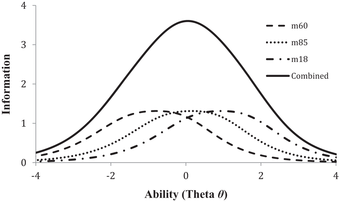
Examples of three item information functions.
A set of items contributes information cumulatively to the total test information of a scale, which can be graphed as its test information function (TIF). The solid line plotted in Figure 3 shows the TIF for the three combined IIFs. Just as an item is more sensitive in one region of the latent dimension than other regions, a collection of items with similar difficulties maximizes information in that specific region. The addition of more items with roughly equivalent difficulty increases test information in the form of precision in this region of the construct, but gains little sensitivity to estimate persons at more distant levels of ability. The TIF for such a scale would be highly peaked and narrow. Note that a concentration of items within a limited range of difficulty may be quite desirable, depending on the intended uses of the scale (Embretson & Reise, 2000). For example, in a brief instrument to screen for suicide lethality, adding a high-difficulty item such as “I see very few reasons to go on living” would presumably add precision in the high-risk range of the latent dimension, where accuracy is needed; whereas an easy item such as “I feel sad from time to time” would probably contribute little to the usefulness of the scale for its intended purpose. Alternatively, researchers may desire an instrument that is as precise as possible through the broadest range of abilities. In this case, the TIF curve would be flattened with thicker tails. These examples bring us to a critically important point that deserves special emphasis: To shorten a subscale, when selecting the final subset of items from a larger pool that meets initial criteria, it is critically important to consider the intended purpose of the scale. Final selection of items and subscale length should be based on item difficulty, desired bandwidth, and total information commensurate with this purpose. Selection based solely on CTT criteria as typically applied in counseling psychology research (e.g., items with highest factor loadings) is unlikely to achieve these goals. (For an elaboration of these principles, see Embretson & Reise, 2000).
The purpose of the EMC/RSEE subscales, including Factor 2, was to provide as broad an evaluation of the underlying constructs as possible, with good sensitivity throughout the full range of person ability. In practical terms, this can be achieved by viewing the difficulty levels in Table 1 as analogous to rungs on a ladder. The researcher’s goal, given this predetermined purpose of the scale, is to select a target set of items whose rungs are neither too close nor too far apart in terms of difficulty and also span the widest range of the underlying contrast (Bond & Fox, 2007; de Ayala, 2009). CTT methods can be used to estimate item difficulty, but these estimates are always sample specific. In contrast, the “sample free” estimates of IIF for an item and TIF of a scale are critical indices of performance, which underscore another advantage of IRT methods not available through CTT.
Applying these principles to the initial difficulty values shown in Table 1 (fourth column), we decided first to retain the most and least difficult items overall, m18 and m60, respectively (i.e., the top and bottom ladder “rungs”). Thus, we preserved the maximum possible range of difficulty bandwidth of the retained items. Next, it was apparent that eight items (m35-m66) spanned a gap only 0.30 logits (−0.19 to +0.09). We retained the most and least difficult items in this cluster. Among the five items in the middle of this span, we dropped three that tapped concerns about English proficiency (m13, s01, m49), because other items tap this content. We dropped m26 because of its length and complexity, and m79 because we were concerned that an item equating religion and superstition was potentially too offensive. Item m85 was retained because it tapped unique content relative to other items retained, and because concerns among White people about their population level relative to U.S. immigrants is a topic frequently discussed in the news. Similar to recalculation of Infit and Outfit, after removing each item, difficulty coefficients for the remaining items were recalculated, because values of remaining items shift after an item is removed. After recalculation, we continued the sequence of identifying closely spaced clusters of difficulty and choosing items to retain or discard based on content coverage. After the decisions described above, the closest remaining pair in difficulty, items m10 and m66, seemed quite conceptually unique.
At this point, our analysis shifted to a consideration of total test information, which is equal to the reciprocal of the squared standard error of estimate (SEE) for all persons in the sample. (SEE is the conceptual corollary in IRT to concept of test reliability in CTT. Lower SEE corresponds to greater precision, that is, higher “reliability.”) Graphically, total information is the total area under the TIF curve (de Ayala, 2009), but typically, scale development researchers using IRT will be more interested in the shape of the TIF curve than its area. Researchers guided only by CTT principles typically decide to stop shortening a scale when the deletion of further items would cause an unacceptable decrease in internal reliability. For researchers guided by IRT, the “how many items is too few?” question is reframed instead by Embretson and Reise (2000) as a question of inspecting the TIF plot in the range of θ (i.e., person ability) of most interest to the researcher, and asking “how much information is high enough?” (p. 270). One benchmark they suggest is an information value of 10.0, which corresponds to a SEE of 0.31, and thus a conventional reliability coefficient in CTT terms of .90. Figure 4 shows the TIF curve plotted by WINSTEPS for the 10 items retained for Factor 2 (solid line labeled “IRT”). The output used to create this plot indicated that the curve exceeded an information level >10.0 in the range of −0.97 to +1.20 logits, which we deemed to be a sufficiently broad interval. Thus, we chose not to delete further items, and we terminated the selection process.
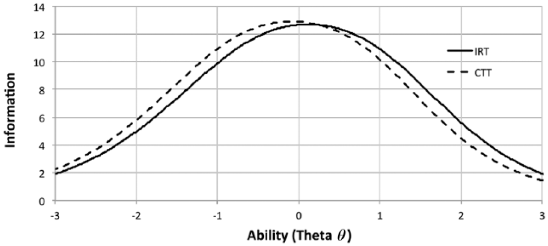
Comparison of test information functions for Factor 2 subscale using IRT versus CTT methods.
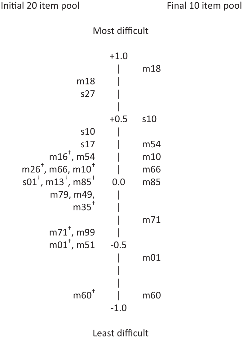
The last column in Table 1 shows the final item difficulties for the 10 items selected that provided the best spread of item sensitivity and content coverage for Factor 2. For contrast, the 10 items with highest factor loadings are flagged with a † in the first column of Table 1. In counseling psychology scale development research guided only by CTT principles, these flagged entries would have been selected for a 10-item subscale derived from Factor 2. Note that only 6 of the 10 items actually selected on the basis of IRT criteria would have been selected using the traditional criteria of highest factor loading to select 10 items, and that 1 of these (m16) has significant sex-based DIF. Figure 5 provides a vertical plot of the difficulty levels of the 20 items that passed initial screening for Factor 2 unidimensionality. Figure 5 shows that, relative to the 10 flagged items on the left that would have been selected based on CTT criteria, the 10 items actually selected for Factor 2 shown in the right half of the figure have two desirable features given the purpose of the subscale: (a) The highest and lowest “rungs” of difficulty are retained, thus preserving the full range of scale difficulty, and (b) the eight items between the most and least difficult generally provide good spacing of intermediate difficulties. Of course, preserving the maximum range of item difficulty cannot be guaranteed when selecting the 10 items with highest factor loadings.
Item difficulties for Factor 2 before and after final item selection.
When researchers select items with difficulty spaced as equally as possible, as we did for the EMC/RSEE, in most cases, the resulting TIF will still be markedly peaked due to the considerable overlap of difficulty among items and concentration of this overlap in the central region of θ. However, equal spacing, all other aspects being equal, should result in a flatter and broader TIF curve than the curve produced by the same number of items selected without attention to difficulty spacing. (Note that a polytomous item with wider spacing of its constituent category difficulties contributes more to flattening the overall TIF than an item with closely spaced category thresholds.) Figure 4 compares two TIF curves. The solid line labeled IRT is the TIF for the 10 items selected for EMC/RSEE Factor 2. The dashed line labeled CTT indicates the TIF for the 10 highest loading items. As expected, the IRT curve is slightly flatter and broader than the CTT curve. Most importantly, the CTT curve is shifted to the left relative to the IRT curve, and the IRT curve is more symmetrical around the midpoint of θ than the CTT curve. This shift is due primarily to the inclusion of three items (m18, s10, and m54) in the IRT version that have greater difficulty than the most difficult item that would have been selected for Factor 2 through CTT methods (see also Table 1 and Figure 5). Thus, the IRT version of Factor 2 is more balanced, whereas the CTT version is relatively more sensitive to respondents who express lower and more benign levels of the attitudes captured by Resentment and Cultural Dominance. Because we are interested in assessing the fullest possible range of these attitudes, including fairly extreme attitudes of resentment and dominance, we view the balanced sensitivity of the IRT version as an important advantage.
A similar process was applied to reduce the 25 items initially assigned to Factor 1. Six had problems with underfit, four had significant DIF for men and women, and two had disordered category thresholds. Of the 13 remaining items, three were discarded due to closely spaced difficulty and content overlap. Thus, 10 items were retained for Factor 1 and, also by coincidence as with Factor 2, only six of these items overlapped with the 10 highest loading items that would have been selected using CTT methods. Before moving to the next section, it should be noted that after winnowing items through the processes described in the proceeding sections, it may become necessary to “return to the drawing board” because the remaining item pool is insufficient. There are at least three reasons why generating and testing new items may be necessary: (a) a failure to achieve sufficient unidimensionality, or the subset of items that is unidimensional is so small that one or both of the next two problems become evident; (b) a large gap in difficulty needs to be spanned with new items (e.g., a pair of “ladder rungs” are too far apart); or (c) bandwidth is restricted, requiring new items with greater or lesser difficulty. We believe that careful use of focus groups at the outset helps minimize risk that the initial item pool turns out to be insufficient.
Evaluating Performance of the Response Scale
Subscale scores for the EMC/RSEE are derived by calculating the mean of items (after reverse keying) that comprise the subscale. One of the most useful features of the Rasch model relative to other IRT approaches is that it provides information about how a measure’s response scale functions. WINSTEPS 3.80 software produced the data shown in Table 2, which can be helpful in deciding whether a Likert-type scale has too many or too few response points. The percentage of students who chose a particular response category is shown in the top row. Thus, for example, only 2% of the sample selected strongly disagree, and only 5% selected moderately disagree, on average, for the 10 items of Factor 1. In addition, Rasch–Andrich thresholds are provided to indicate the person-ability levels that define the transitions between two adjacent responses for the factor as a whole. For example, persons just above an ability level of −1.40 logits on Factor 2 were more likely to choose a response of moderately disagree than strongly disagree, whereas those whose ability ranged from just above −0.74 logits to just below −0.10 logits were most likely to choose slightly disagree. For a full scale, in contrast to individual items, these thresholds are referred to as step calibrations. In much the same way as the finding of disordered thresholds suggests a poorly functioning individual item, disordered step calibrations for an entire subscale suggest a poorly functioning response scale for that factor. Table 2 shows that Factor 2 exhibited disordered step calibration because the transition between moderately agree and strongly agree (1.08) is actually lower in difficulty than the step calibration between slightly agree and moderately agree (1.16). In practice, this means that the additional point added to a student’s score when she or he chooses strongly agree versus moderately agree for any of the items of Factor 2 actually increases error and reduces precision in the subscale total score. The problem can be rectified by combining neighboring response points across the disordered step calibrations, that is, by recoding strongly agree responses for Factor 2 so that they are equivalent to moderately agree responses.
Response Scale Functioning for EMC/RSEE Factors 1, 2, and 3
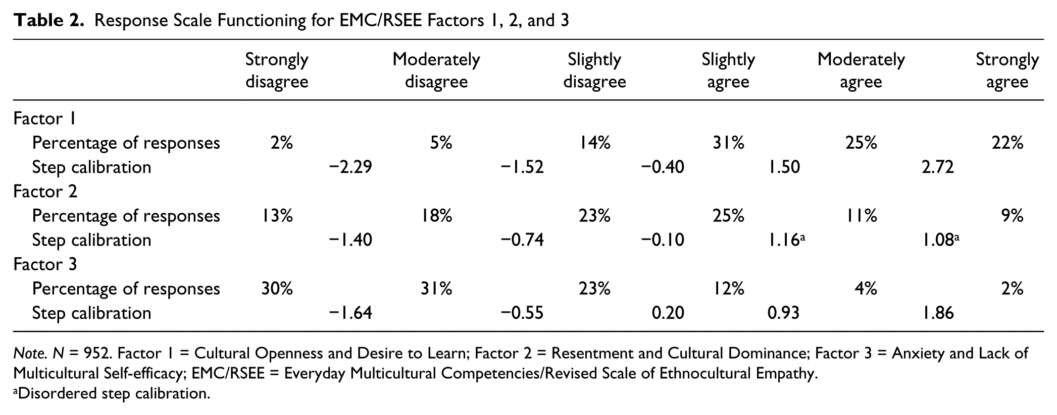
Note. N = 952. Factor 1 = Cultural Openness and Desire to Learn; Factor 2 = Resentment and Cultural Dominance; Factor 3 = Anxiety and Lack of Multicultural Self-efficacy; EMC/RSEE = Everyday Multicultural Competencies/Revised Scale of Ethnocultural Empathy.
Disordered step calibration.
Guidelines from Linacre (1999) and also recommended by Bond and Fox (2007) suggest that, in an optimally functioning response scale, the step calibration distance between adjacent categories should be at least 1.4 logits, but not more than 5 logits. Values less than 1.4 suggest neighboring categories that could be combined, and calibration distances greater than 5.0 suggest a gap too wide, and thus the need for a more fine-grained response scale. In addition, a particular category may introduce “noise” in terms of underfit, similar to a poor fitting individual item. Underfit mean square coefficients are not shown in Table 2, but only one was greater than the recommended cutoff of 2.0 for mean squares Outfit (Factor 3, Category 5 and 6 outfit mean square = 2.19). Bond and Fox provide further suggestions and emphasize the importance of considering multiple sources of information when deciding whether to collapse response scale categories. Based on these recommendations, we adopted the following subscale scoring modifications. Due to disordered step calibration for Factor 2, all items were recoded “(6 = 5)” to combine strongly agree and moderately agree. Because of low category frequency (<3%) and small step calibration distances (<1.0 logits), we combined strongly disagree and moderately disagree for Factor 1 (coding 1 = 2). For the same reasons, and because of significant category underfit for Factor 3, we combined strongly agree and moderately agree (coding 6 = 5).
Empirical Test of the Benefits of IRT
We began by analyzing the effects of combining response scale points for Factors 1, 2 and 3. Table 3 shows that although the 5-point versions of subscales had less variance than the 6-point versions, as would be expected, both internal reliability and retest reliability were virtually unchanged (and slightly improved in five of the nine comparisons). These findings suggest that the reductions in variance, which ranged from 1.7% (Factor 3 at Time 2) to more than 22% (Factor 2 and Time 1), primarily eliminated error variance (here, for the moment, we apply the CTT framework). To further test the effect of collapsing categories, we examined correlations with measures included by Mallinckrodt et al. (2014) to estimate the construct validity of the EMC/RSEE: (a) the three subscales of the Miville-Guzman Universality-Diversity Scale–Short form (MGUDS-S; Fuertes, Miville, Mohr, Sedlacek, & Gretchen, 2000), and (b) the Openness to Diversity Scale (Pascarella, Edison, Nora, Hagedon, & Terenzini, 1996). Table 4 compares correlations with these construct validity measures for versions of EMC/RSEE subscales for Factors 1, 2, and 3. The top row shows correlations for the traditional CTT subscales of Factors 1 and 2 composed of the 10 items with the highest factor loadings. (For Factor 3, the 7 items selected based on IRT methods were also the highest loading CTT items.) Next, correlations are shown for factors constructed using IRT criteria with the 6-point response scale scoring preserved. The last row in each section shows the 5-point subscale scoring that we suggest for the EMC/RSEE. Thus, each row reading down within a section shows an incremental advantage conferred through using IRT criteria to construct an instrument. A clear general trend of higher correlations is shown (10 of 12 comparisons), with a mean increase of more than 4%. Results for Factors 1 and 2 suggest that much of the improvement occurred through item selection, although Factor 2 also clearly benefited from collapsing the response scale points.
Effect on Subscale Mean, Variance, and Reliability of Collapsing 6-Point to 5-Point Response Scales for EMC/RSEE Factors 1, 2, and 3
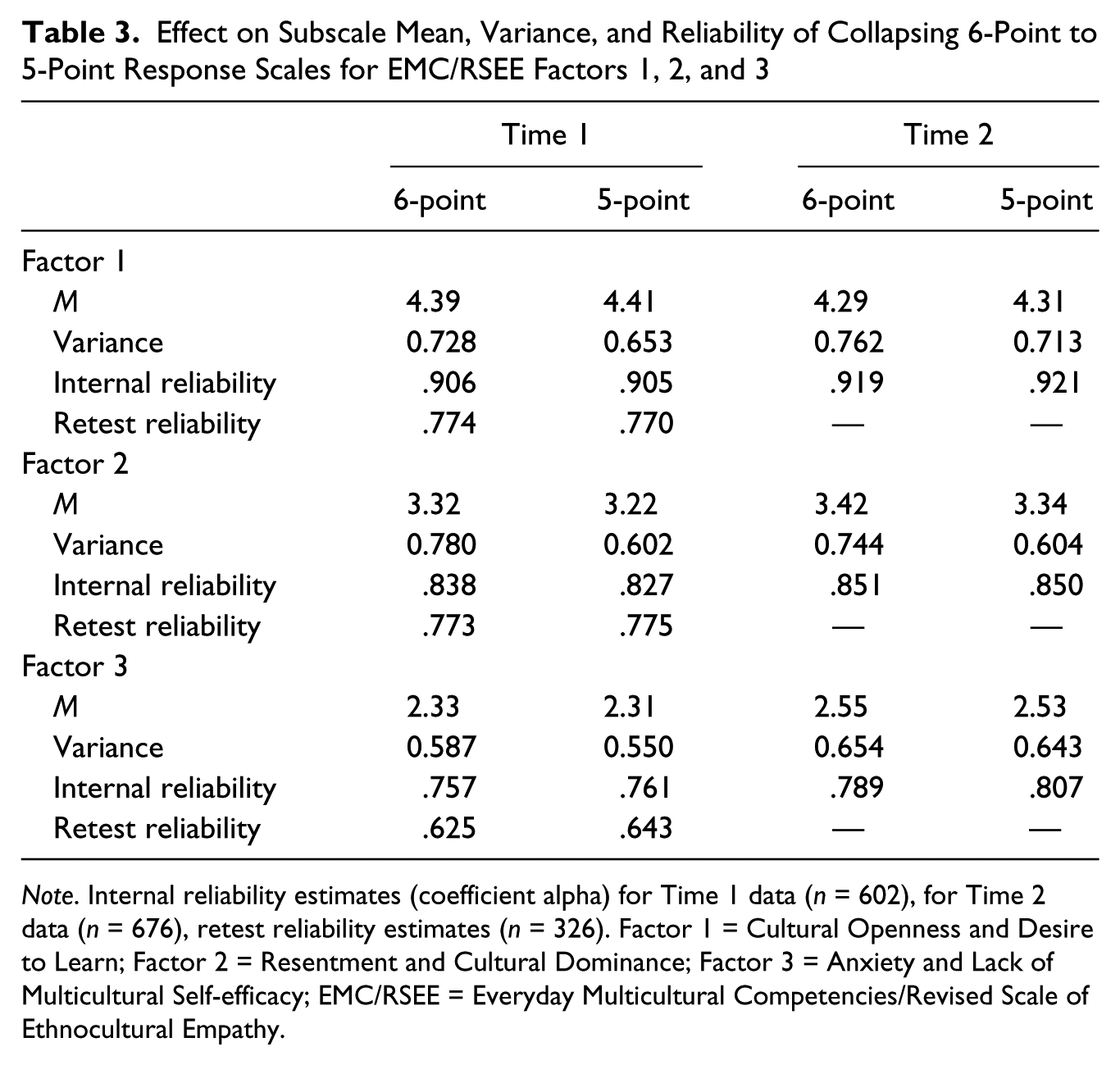
Note. Internal reliability estimates (coefficient alpha) for Time 1 data (n = 602), for Time 2 data (n = 676), retest reliability estimates (n = 326). Factor 1 = Cultural Openness and Desire to Learn; Factor 2 = Resentment and Cultural Dominance; Factor 3 = Anxiety and Lack of Multicultural Self-efficacy; EMC/RSEE = Everyday Multicultural Competencies/Revised Scale of Ethnocultural Empathy.
Convergent Validity Correlations for Versions of EMC/RSEE Factors 1, 2, and 3 at Time 2
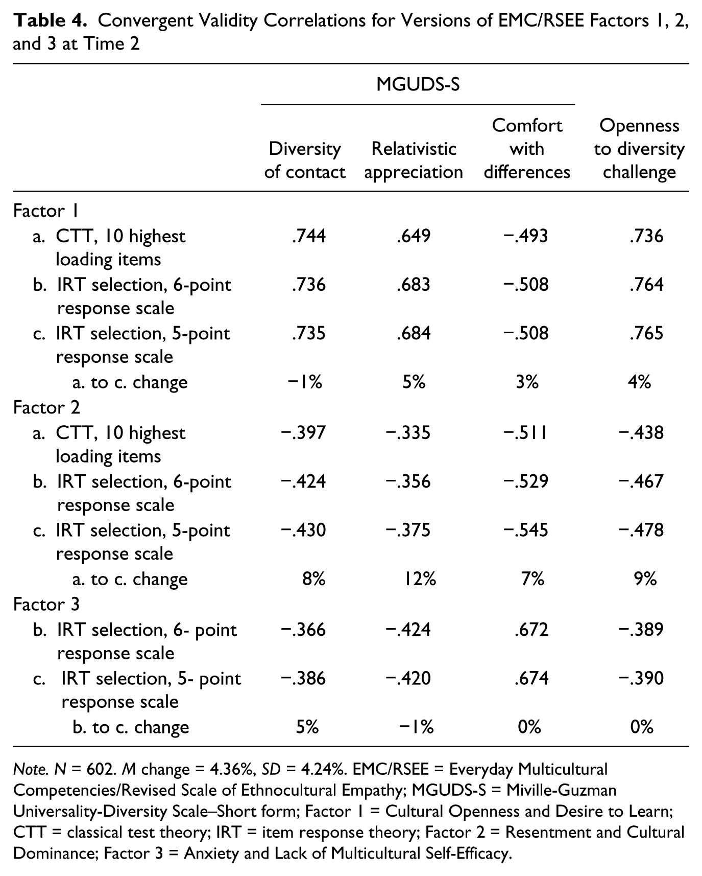
Note. N = 602. M change = 4.36%, SD = 4.24%. EMC/RSEE = Everyday Multicultural Competencies/Revised Scale of Ethnocultural Empathy; MGUDS-S = Miville-Guzman Universality-Diversity Scale–Short form; Factor 1 = Cultural Openness and Desire to Learn; CTT = classical test theory; IRT = item response theory; Factor 2 = Resentment and Cultural Dominance; Factor 3 = Anxiety and Lack of Multicultural Self-Efficacy.
Conducting IRT analyses as a basis for selecting items adds extra steps to the instrument development process, and may be a cause for concern when readers note how little difference there seems to be in the IRT and CTT information curves shown in Figure 4. In other words, it is understandable to ask, “Does all this extra work make a practical difference?” The final analyses we conducted represent an empirical attempt to answer this question.
When IRT methods are used to maximize bandwidth, the result should be scales with improved sensitivity to change or differences between groups. To test this advantage empirically, we assigned students to three groups based on their answer to a Time 1 multiple-choice item about how racially and ethnically diverse their high school had been. We reasoned that students with more diverse high school experiences should have higher levels of everyday multicultural competencies. Table 5 shows the results of this comparison. In the last column, the top value of each pair shows effect size estimates for EMC/RSEE Factors 1, 2, and 3, constructed using CTT methods (i.e., highest loading items). The second row of each pair shows results for the actual EMC/RSEE scales based on IRT criteria. For Factors 1 and 2, the significance levels are lower and F values are greater for the IRT scales. (However, note that for Factor 2, partial η2 rounds to .004 for both IRT and CTT subscales, even though the IRT effect size is larger.) Recall that the items for Factors 1 and 2 are different for CTT and IRT versions, whereas the only difference for Factor 3 is use of a 5-point versus 6-point response scale. Although none of the first three factors were significantly different based on high school diversity, there were strong differences for Factor 4, Empathic Perspective Taking, and differences that approached significance for Factor 5, Awareness of Contemporary Racism and Privilege. A one-way MANOVA for all six EMC/RSEE subscales suggested significant differences based on high school diversity, F(12, 1190) = 1.82, p = .041, η2 = .018. However, the same analysis conducted after substituting the first three CTT subscales for the IRT subscales was not significant, F(12, 1190) = 1.73, p = .055, η2 = .017. Thus, the IRT-based subscales made a consequential difference, relative to CTT subscales, in this analysis of group differences in high school diversity.
Comparison of Sensitivity to Group Differences of EMC/RSEE Factors With and Without IRT Selection Criteria
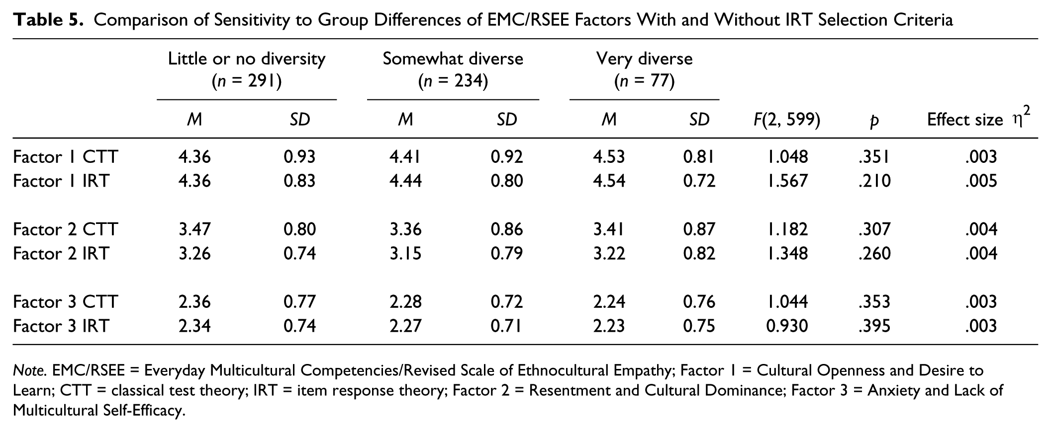
Note. EMC/RSEE = Everyday Multicultural Competencies/Revised Scale of Ethnocultural Empathy; Factor 1 = Cultural Openness and Desire to Learn; CTT = classical test theory; IRT = item response theory; Factor 2 = Resentment and Cultural Dominance; Factor 3 = Anxiety and Lack of Multicultural Self-Efficacy.
For our final comparison, we assessed change over the 5-week period from Time 1 to Time 2, which occurred in the last half of Fall semester. The first semester of university education may be a time of profound change for first-year students (Lopez & Gormley, 2002), so we focused the analyses on participants aged 17 or 18 in the retest sample. (Our survey asked about age, but not class status.) Table 6 shows the results of these repeated measures comparisons. The top row of each pair shows the results for the “traditional” method of forming subscales recommended based on CTT. The second row shows the results for the three corresponding EMC/RSEE subscales constructed with additional criteria derived from IRT. Table 6 shows that, in every case, the IRT subscales yielded higher estimates of effect size. It is interesting to note that the bandwidths for CTT and IRT in Factor 1 are the same because both methods result in selection of the most and least difficult items, but for Factor 2 the bandwidth is wider for IRT. Table 6 shows dramatic differences for the two forms of Factor 2, with the CTT version not statistically significant and the IRT version significant at p < .0001. Clearly, the expanded bandwidth and more balanced test information sensitivity for the IRT subscale in the most difficult region of the latent construct helped this EMC/RSEE subscale detect change in the last half of the semester. Note that change is in the direction of significantly intensifying negative attitudes captured by Factor 2.
Comparison of Sensitivity to Time 1 and Time 2 Change of EMC/RSEE Factors, With and Without IRT Selection Criteria
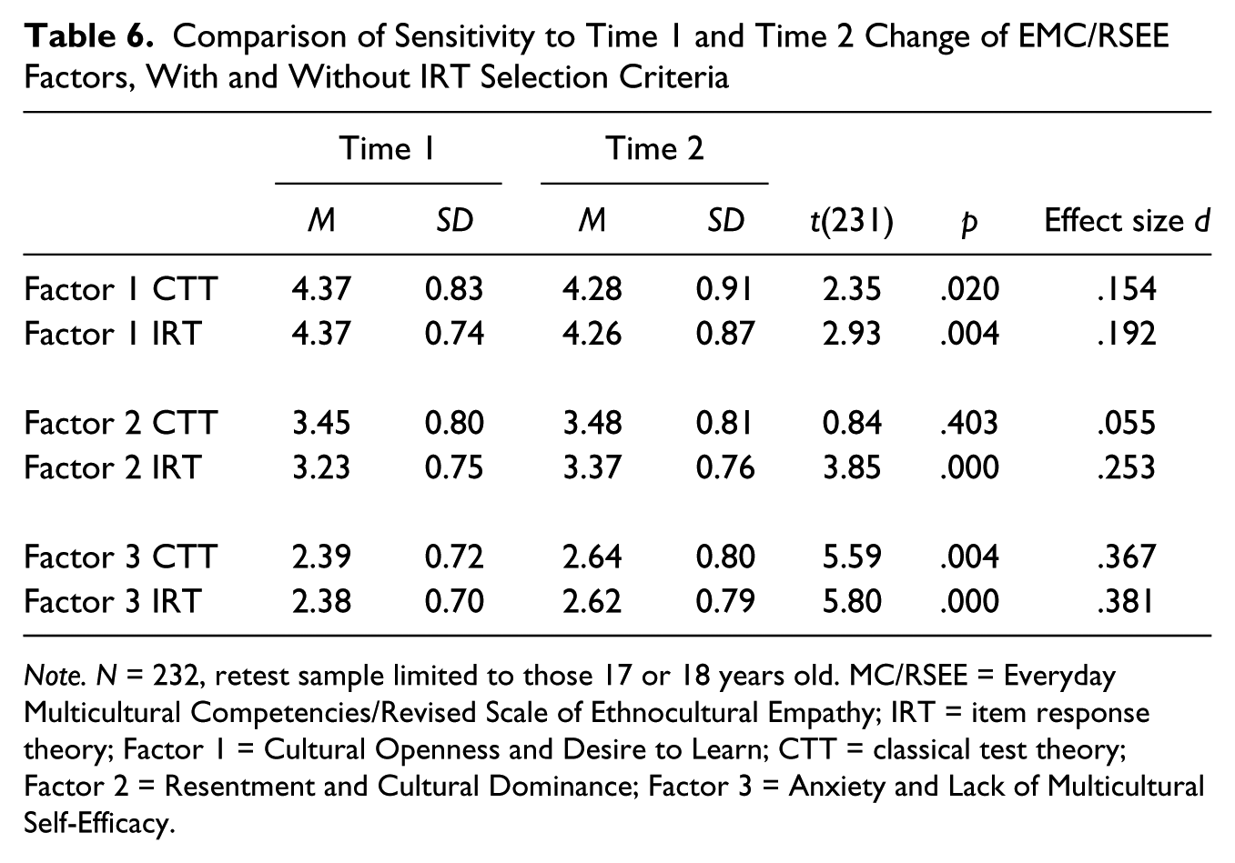
Note. N = 232, retest sample limited to those 17 or 18 years old. MC/RSEE = Everyday Multicultural Competencies/Revised Scale of Ethnocultural Empathy; IRT = item response theory; Factor 1 = Cultural Openness and Desire to Learn; CTT = classical test theory; Factor 2 = Resentment and Cultural Dominance; Factor 3 = Anxiety and Lack of Multicultural Self-Efficacy.
IRT and CFA
After EFA and assignment of items to subscales, it is important to conduct a CFA with a new sample to support the proposed subscale structure. However, there is some controversy about how to conduct the CFA. Worthington and Whittaker (2006) recommended using each item as an observed indicator of its latent factor. They caution, citing Cattell (1974), as well as Bandalos and Finney (2001), that “item parcels mask the true relationships among items in the scale . . . in addition, model misspecification may be hidden when using item parceling” (p. 831). In contrast, other experts point to problems introduced by not using item parcels. For example, Floyd and Widaman (1995) warned that subscale structure can be very difficult to confirm with individual item indicators when the subscales contain more than 5 to 8 items. The problem is that pairs or small clusters of items often share variance unrelated to the parent latent factor based on idiosyncrasies of content or wording. For example, all negatively worded items across factors may share significant covariance. In a subscale assessing depressive symptoms, two items tapping changes in weight and appetite may have highly correlated errors. Under these circumstances, fitting a CFA model to the data is problematic. Floyd and Widaman observed that
It is difficult to identify, on an a priori basis, all of the necessary correlated error terms if the indicators in the analysis are items from a long questionnaire . . . Thus, it may be unreasonable to expect that lengthy questionnaires with many items assessing each factor will show satisfactory solutions when the individual items are submitted to confirmatory factor analysis. (p. 293)
IRT methods can resolve this dilemma. Screening items to ensure unidimensionality, as previously described, should address the important cautions Worthington and Whittaker (2006) highlighted about model misspecification and item parceling. If assumptions about unidimensionality in each subscale have been met through IRT screening, researchers can use item parcels as indicators of latent factors, thereby avoiding the problems of CFA model fit with individual items mentioned by Floyd and Widaman (1995). A further advantage is that a model with the recommended three item parcels per latent factor (Kline, 2011) has fewer parameters to estimate and therefore requires fewer subjects than a model based in individual item indicators.
For the CFA conducted on a holdout sample of the 952 independent observations, Mallinckrodt et al. (2014) used a model with three parcels of items as indicators for each of the six factors of the EMC/RSEE. They reported this model provided an adequate fit to the data, comparative fit index (CFI) = .950. However, a model we tested for this example with 48 individual items as indicators of the six factors provided a much poorer fit, CFI = .884. Hu and Bentler (1999) suggested that CFI values >.95 are desirable.
Discussion
Since the first attempts to introduce IRT to our field nearly two decades ago (Fox & Jones, 1998; Harvey & Hammer, 1999), these methods still are rarely used in counseling psychology research. (For exceptions, see del Prado & Church, 2010; McAleavey et al., 2012.) Following Wampold’s (1998) suggestion, we attempted to promote greater adoption of IRT methods by providing readers with a step-by-step empirical example relevant to counseling psychology research. Findings suggest three sets of advantages conferred by adding IRT methods in scale development research.
First, IRT methods permit an analysis of response scale performance. The Rasch model approach provides extremely useful information. Disordered category thresholds for individual items and disordered step calibrations at the level of full subscales inject error variance. This problem can be avoided by deleting individual items or by combining neighboring response categories for a full subscale. The full response scale can be used for all items, then response categories can be combined at the stage of data analysis. This allows researchers to use different item-scoring schemes, each best suited for individual subscales, without adding to the complexity of multiple response scales for respondents. For example, instead of presenting different 5-point and 6-point Likert-type scales for alternating EMC/RSEE items, because the 6-point scale performed well for three of the six subscales, and to preserve simplicity in presenting the instrument, the 6-point format was retained for all EMC/RSEE items. Recoding is accomplished after data collection. Rasch model IRT analyses can suggest the optimal number of response points for a specific latent construct, and avoid introducing error through superfluous categories (Fox & Jones, 1998).
Results of this study suggest that collapsing poor-performing response categories results in improved scale performance. Despite reduction in total subscale variance after collapsing categories, correlations with other measures used to estimate construct validity increased (see Table 4). Although these increases were modest, we believe this improvement in reduced measurement error is well worth the effort, especially because IRT confers other benefits. Monte Carlo research suggests that the optimal number of Likert-type response points is probably between four and seven (Lozano, Garcia-Cueto, & Muniz, 2008). A field study that compared a variety of 2-point through 11-point Likert-type formats reported that reliability increased up through the 7-point format, then leveled off (Preston & Colman, 2000). An important assumption of all response formats is that pairs of neighboring responses represent equidistant measurement intervals. Recent research suggests that respondents have great difficulty making meaningful distinctions between vague frequency-based response points such as sometimes and often (Bocklisch et al., 2012). IRT methods can be used to check on the validity of this important measurement assumption.
It is tempting to speculate how performance of measures frequently used in counseling psychology research might be improved through an IRT analysis of response scale performance. A recent IRT study of data from over 1,700 clients seen at a wide range of community clinics and university counseling centers reported that the 7-point response format of the WAI (Horvath & Greenberg, 1989) performs very poorly (Mallinckrodt & Tekie, in press). Correlations with counseling outcome and process variables were improved when the lower response points were collapsed. IRT methods described here were used to create a 16-item Brief Alliance Inventory (BAI) with maximum bandwidth and information value. The BAI performed better in many respects than two widely used alternative brief alliance measures, and as well in some respects as the full 36-item WAI.
The second important advantage conferred by IRT is the capacity to introduce DIF analyses as a critical element in item selection. In scale development research, comparisons of mean differences between men and women (or members of different social identity groups, such as race) are routinely reported, but readers should understand that a finding of no significant mean differences provides absolutely no information about the operation of bias in the items. In fact, the results of this study illustrate how an item that exhibited no significant mean difference for men and women exhibited highly significant DIF. Conversely, items with very different mean scores for men and women may not be biased for the purpose of assessing relative levels of a trait or an attitude. It is disquieting to consider that most of the instruments used in counseling psychology research have never been thoroughly investigated for the possibility of sex (or other) differential item functioning bias.
Finally, the third advantage available through using IRT methods is the possibility of selecting a final set of items that maximizes test information of a scale in the region of greatest interest, thereby increasing sensitivity to detect group differences or change over time. However, depending on the construct, the effort to maximize bandwidth must be tempered by sensitivity to edit or exclude items that respondents may find too offensive, as was the case for the EMC/RSEE. The bandwidth of a psychological instrument refers to its sensitivity for differentiating individuals at ability levels through the full range of a latent construct (Embretson & Reise, 2000). Selecting items for final inclusion in a subscale with careful attention to expanding the range of difficulty to be as wide as possible has the effect of both “raising the ceiling” and “lowering the floor” with respect to the range of resulting scores. When researchers have no special interest in a particular restricted range of person ability, selecting items with intervals in difficulty as evenly spaced as possible flattens and broadens the TIF. A useful analogy comes from the methods used by ceramic artists to accurately measure the temperature of their kilns, which often must exceed many hundreds of degrees. Although expensive digital measuring equipment is available, a reliable, less expensive alternative is provided by pyrometric cones. A numbered sequence of cones each is composed of a slightly different ceramic mixture, known to melt at a precisely calibrated temperature. A specific cone melts through only a relatively narrow range of temperature, but through careful selection of a range of cones with different melting points, the potter watches as the cones sag one by one to determine the precise temperature (P. P. Heppner, personal communication, October 19, 2012). To continue the analogy, a single item that uses a 5-point response scale actually introduces four “cones” of differing sensitivity, one for each of the 0.50 probability thresholds between response points.
Therefore, given our belief in the advantages of IRT, we disagree with one particular set of best practices identified by Worthington and Whittaker (2006):
Generally, when a factor contains more than the desired number of items, the researcher will have the option of deleting items that (a) have the lowest factor loadings, (b) have the highest cross-loadings, (c) contribute the least to the internal consistency of the scale scores, and (d) have low conceptual consistency with other items on the factor. The researcher should avoid scale-length optimization that degrades the quality of the factor structure, factor intercorrelations, item communalities, factor loadings, or cross-loadings. (p. 823)
Certainly, this recommendation is a common practice in counseling psychology research based on CTT assumptions about true scores, measurement error, and scaling derived from summed scores. Generally, under assumptions of CTT the goal is to select a subset of unweighted items that will provide a summed score that is the most reliable possible estimate of an individual’s hypothetical true score. However, as discussed previously, IRT emphasizes the performance of individual items for accurately placing individuals along an hypothesized latent dimension. Consequently, instead of selection based on CTT assumptions about item-factor loading and maximization of internal reliability, IRT criteria emphasize item selection to increase unidimensionality and maximize the total information value of a scale through attention to item difficulties. Note that, in this study, following the CTT-based highest factor loading criteria would have resulted in inclusion of an item with significant sex DIF. Table 1 shows that under CTT criteria, the 10 highest loading items for Factor 2 would provide a bandwidth (Item m60 to Item m16) that ranges only from −0.87 to +0.20 logits (see column 4), whereas the bandwidth achieved with IRT criteria (Item m60 to Item m18) ranged from −0.94 to +0.95 logits. In other words, IRT criteria produced a Factor 2 subscale that spanned 1.89 logits in bandwidth, whereas CTT criteria with span would have been only 1.07 logits. Moreover, Figures 4 and 5 highlight a problem with using CTT criteria, apart from restricted bandwidth. Note how many of the flagged (i.e., 10 highest loading) items shown in the left half of the Wright diagram (Figure 5) cluster in a small central range of difficulty/ability. Table 1 shows that 7 of the top 10 highest loading items are found within a narrow range of difficulties, −0.19 to +0.20 logits. This clustering concentrates the information value still further than the narrowed bandwidth. An analogy would be the lack of information about kiln temperature a potter would have who, instead of having 10 cones evenly spaced at 100 degree intervals between 600 and 1500 degrees, has cones at 600, 700, and 800 degrees, plus 7 others densely spaced from 900 to 1000. After the 1000 degree cone melts, there would be no indicator for further temperature increase, just as there is no flagged item in the left half of Figure 5 above +0.20 logits.
We believe that developing scales with wide bandwidth and broadly sensitive information value are objectives that should be considered at least as important as maximizing internal reliability. These goals are in opposition to a degree because items with the highest and lowest difficulty level often exhibit lower item total correlations than items with midrange difficulty. Very easy and very difficult items are most sensitive to discriminating respondents at extreme levels on the latent construct of interest. These individuals are often of great interest to counseling psychology researchers, for example, the most depressed clients, those with the poorest working alliances, or students experiencing the greatest amount of stress. A study of breast cancer survivors found that the significant correlations between social support and adjustment observed in the entire sample could be accounted for entirely by women in the lowest quartile of social support scores. For the women in the highest three quartiles, social support was not significantly related to adjustment (Mallinckrodt, Armer, & Heppner, 2012). The authors questioned the sensitivity of the social support scale used in their study to differentiate among women through the full range of support they experienced.
In outcome research, interventions are unlikely to affect all individuals in a population equally. For example, the same type of psychotherapy in-session process comment may generally improve the working alliances of clients whose alliance was very poor before the intervention, have no effect on clients with midrange alliances, and actually cause a deterioration in initially strong alliances. (Here we assume correction for regression to the mean.) If the measure of alliance used by researchers lacks items sensitive to differences at the lower end of the range, but is stocked with items that tap differences between good and very good working alliances, the researchers may conclude that the process intervention was generally not helpful—or worse, that it is harmful—mistakenly basing this conclusion on a measure without sufficient sensitivity to assess all segments of “ability” in the population of interest (Mallinckrodt & Tekie, in press). Selection solely on the basis of highest factor loadings may exclude items that are particularly sensitive at detecting the relatively small proportion of individuals with extreme scores in either tail of the distribution—who may nevertheless be of great theoretical interest.
Readers may question whether the effort and time required to incorporate IRT criteria in their instrument development research have any substantial practical benefit. We believe the results shown in Tables 3 to 6 provide examples that answer this question in the affirmative. This study suggests that IRT methods can be used to reduce error variance (Table 3), increase correlations with variables of interest (Table 4), increase sensitivity of scales to group differences (Table 5), and increase sensitivity to detect change over time (Table 6). As Table 6 shows, the additional items balancing the sensitivity of Factor 2 in higher rungs of the construct were able to detect an increase in Factor 2 in the second half of students’ first Fall semester, whereas the CTT-based items suggested no change. This increase in Resentment and Cultural Dominance for first-year White students in their first semester is disturbing, and suggests an intensification of negative attitudes, particularly at the high end of difficulty shown in Table 1. A CTT scale relatively less sensitive to extremely negative attitudes would not have detected change in those attitudes. IRT-based item selection has identified a trend of change in this sample that needs further study.
We hope that the empirical demonstration presented in this study persuades readers that using Rasch IRT methods in scale construction is well worth the additional effort. Our treatment of the topics has been necessarily brief, but excellent introductory descriptions are available to help researchers acquire these important skills (cf. Bond & Fox, 2007; de Ayala, 2009; Doucette & Wolf, 2009; Embretson & Reise, 2000). The steps presented in the appendix are intended to supplement Worthington and Whittaker’s (2006) recommendations, by expanding their list of suggestions to include focus groups at the “front end” of item generation and IRT methods at the “back end” to guide final item selection. After the first goal of describing the advantages of using focus groups to generate a broad item pool, the second goal of this article was to demonstrate for readers unfamiliar with IRT that these methods can significantly improve the item selection stage of instrument development. The two goals work hand-in-hand, because IRT methods operate best when a broad and representative “universe” of items has been generated for analysis. IRT will not salvage an inadequate item pool, but these techniques can capitalize on the advantages of a broad and comprehensive pool. Our hope is that these suggestions will help improve the quality of counseling psychology scale development research.
Footnotes
Appendix
Declaration of Conflicting Interests
The authors declared no potential conflicts of interest with respect to the research, authorship, and/or publication of this article.
Funding
The authors received no financial support for the research, authorship, and/or publication of this article.
Notes
Author Biographies
References
Supplementary Material
Please find the following supplemental material available below.
For Open Access articles published under a Creative Commons License, all supplemental material carries the same license as the article it is associated with.
For non-Open Access articles published, all supplemental material carries a non-exclusive license, and permission requests for re-use of supplemental material or any part of supplemental material shall be sent directly to the copyright owner as specified in the copyright notice associated with the article.