
Abstract
This study aims to empirically test the immunity effect on the frequency distribution of household victimizations. To clarify the immunity effect, the statistical construction of zero-inflated models is reviewed and compared with that of non-zero-inflated models. The Benjamini and Hochberg correction is used to address the limitation of p values in multiple testing. Compared with the findings from the non-zero-inflated model, two sets of coefficients from the zero-inflated model reveal that there exist more complex and diverse statuses in the process of household victimization than predicted by risk heterogeneity and event dependence. With these findings, this study suggests that zero-inflated models should be introduced and compared with non-zero-inflated models for the clarification of victimization determinants.
Introduction
Since 1990s, the recurrence of criminal victimizations to a small portion of the population has gained growing attention in criminological studies (Deams, 2005; Farrell, 1995; Fisher, Daigle, & Cullen, 2010; Pease, 1998; Turanovic & Pratt, 2014). Earlier academic interest was initiated by findings from the Kirkholt Burglary Prevention Project in Rochdale, England, which revealed the practical benefit of focusing crime prevention efforts on the households that were frequently burglarized (Forrester, Chatterton, & Pease, 1988; Forrester, Frenz, O’Connell, & Pease, 1990). Several follow-up studies designated repetition of victimizations to the same target as repeat victimization (Farrell, 1995; Pease, 1998) and produced a large amount of policy-driven literature on this phenomenon (Deams, 2005). These studies’ main argument was that prior victimization is a good predictor of future victimization, and, therefore, crimes can be more effectively prevented by providing crime prevention resources to those who were repeatedly victimized (Lauritsen & Davis-Quinet, 1995; Osborn, Ellingworth, Hope, & Trickett, 1996; Osborn & Tseloni, 1998; Pease, 1998).
From the methodological viewpoint, repeat victimization has been addressed as an aggregate-level distribution of victimizations that is significantly more dispersed than is expected from the Poisson distribution (Farrell & Pease, 1993; Hindelang, Gottfredson, & Garafalo, 1978; Nelson, 1980; Short, D’Orsogna, Brantingham, & Tita, 2009; Sparks, Genn, & Dodd, 1977). The remaining variance after fitting the Poisson distribution is presented as over-dispersion (Berk & MacDonald, 2008; Osgood, 2000; Paternoster & Brame, 1997). As the Poisson distribution premises a random and independent process to be chosen (Park & Eck, 2013), the existence of over-dispersion in the distribution of victimizations has been identified as an evidence of individual heterogeneity where there is enduring uneven risk of victimization and/or event dependence where the previous victimization elevates the risk of future victimization (Ousey, Wilcox, & Brummel, 2008; Tseloni & Pease, 2003, 2004). Studies from this perspective have been devoted to the clarification of flag (individual heterogeneity) and boost (event dependence) effects (Ousey et al., 2008; Tseloni & Pease, 2003, 2004) and the identification of determinants of these two effects (Fisher et al., 2010; Lauritsen & Davis-Quinet, 1995; Outlaw, Ruback, & Britt, 2002; Tseloni, Wittebrood, Farrell, & Pease, 2004).
While both practical and methodological perspectives have dominated the studies of the frequency patterns of victimizations, two recent studies have initiated new arguments about the analysis of counted number of experienced victimizations. First, through mathematical demonstrations, Park and Eck (2013) showed that the concentration of victimizations on a small number of the population could happen even when there was no individual heterogeneity and event dependence. They named this repetition of victimizations as random repeats and argued that random repeats spontaneously happened during the process of selecting targets (Park & Eck, 2013, p. 403). Second, using the latent class analysis, Hope and Norris (2013) revealed that the existence of excessive zeroes (i.e., nonvictims), in addition to excessive high frequency, was the other reason of over-dispersed victimization counts. They then concluded that the distribution of criminal victimization events cannot be properly analyzed without considering the effect of zero inflation, so-called immunity (Hope & Norris, 2013, p. 572). In sum, both studies have shown that the distribution of victimization counts is the result of more complicating processes than expected by risk heterogeneity and event dependence, and the higher frequency of victimization does not always indicate a higher risk of future victimization.
While random repeat and immunity arguments have been recently proposed in the studies of victimization distributions, diverse statistical models have been already initiated to address the zero-inflation effect on skewed count data distributions (Winkelmann, 2008). In addition, as discussed in the following section, the necessity of considering the immunity effect is that the failure to identify zero-inflation effects causes erroneous identification of random repeats as high-risk repeat victimizations. The main purpose of the present study is to empirically test the immunity effect in the analysis of criminal victimization frequencies. For this purpose, the zero-inflated models are reviewed, and the results from zero-inflated and non-zero-inflated analyses of the 2010 National Crime Victimization Survey (NCVS) data are compared to identify differences between the two analyses. This comparison is expected to clarify the necessity of considering an immunity effect in empirical studies of victimizations and reveal whether the application of zero-inflated models enhances the comprehension of victimization distributions.
Repeat Victimization and Random Repeat
Repeat victimization is generally defined as the recurrence of the same type of crime in the same places and/or against the same people (Farrell, 1995; Pease, 1998). Two important aspects of repeat victimization provide a key to the practical benefits of this phenomenon: (a) Victimizations tend to be concentrated on a relatively small portion of the population (Farrell, Tseloni, & Pease, 2005; Farrell & Pease, 1993; Gottfredson, 1984; Tilley & Laycock, 2002) and (b) the number of prior victimizations is a good predictor of future victimization (Lauritsen & Davis-Quinet, 1995; Osborn et al., 1996; Osborn & Tseloni, 1998; Pease, 1998). Based on these considerations, policies targeting repeat victimization have been portrayed as a practical solution to preventing crimes more effectively and efficiently (Farrell, 2005; Pease, 1998).
Theoretically, the phenomenon of repeat victimization is addressed with the routine activity and lifestyle perspectives. These perspectives argue that the risk of victimization is mainly determined by routines in victim’s lifestyle such as (a) close physical proximity to motivated offenders, (b) exposure to crimes, (c) target suitability, and (d) lack of capable guardianship (Fisher et al., 2010). Studies from these perspectives consistently found that these routine lifestyle factors exercised significant influence on repeat victimization (Cass, 2007; Fisher et al., 2010; Mustaine & Tewksbury, 2007; Schwartz & Pitts, 1995; Tseloni et al., 2004).
Based on these findings, Farrell and his colleagues (2005) have argued that as crime prevention resources are scarce, these resources should be allocated where victimizations are most concentrated. Furthermore, the identification of vulnerable attributes of repeat victims or targets has been presented as another route to the increment of crime prevention effectiveness (Farrell, 2005; Sparks, 1981). This line of thinking has generated several crime prevention projects directed at reducing risk of repeat victimization, including household burglaries (Farrell, 2005; Pease, 1998), domestic violence (Hanmer, Griffiths, & Jerwood, 1999; Lloyd, Farrell, & Pease, 1994), sexual victimization (Breitenbecher & Christine, 1998), and racial attack (Sampson & Phillips, 1992). In England and Wales, for example, studies on repeat victimization have influenced criminal justice policies such as (a) six “roadshows” on repeat victimization (Laycock & Farrell, 2003), (b) a task force in the U.K. central government (Laycock, 2001; Laycock & Clarke, 2001), (c) initiation of repeat victimization liaison officers in 43 police forces (Laycock & Farrell, 2003), and (d) reducing repeat victimization as one of the Home Secretary’s performance indicators (Laycock & Farrell, 2003). Reducing repeat victimization has become the backbone of crime prevention practices in England and Wales (Farrell & Pease, 2001). More broadly, several scholars have posited that one of the most promising areas of research in criminology is understanding and reducing of repeat victimization (Davis, Maxwell, & Taylor, 2006; Deams, 2005; Skogan, 1999).
Contrary to this speculation, Park and Eck (2013) argued that the number of previous victimizations should be cautiously used to identify victims’ vulnerability. They presented two different types of recurrent victimization: repeated victimizations by random chance and those by risk heterogeneity/event dependence. According to their explanation, when one individual is randomly selected for victimization, he or she is not excluded from the pool for the next random selection. Therefore, subsequent victimization can happen to previous victims regardless of their vulnerability (see Park & Eck, 2013). While the frequencies of nonrandom repeat victimizations are reliable sources to estimate victims’ propensities, those of random repeats are not related with the victims’ characteristics, because those who retain a random chance of victimization (= random risk) can be victimized none, one time, or multiple times only by chance. They designated this random multiple victimization as “random repeats” and, with a mathematical demonstration, showed that the amount of random repeats in a given period is determined by the crime rate. This argument indicates that the area with a greater crime rate should exhibit a higher level of random repeats. Theoretically, this argument implies that individuals would have larger chance to be randomly victimized in the area with higher crime rate.
The random repeats argument is also relevant to the structure of a negative binomial model. When the frequency distribution of incidents is over-dispersed than expected by a random and independent Poisson process, an over-dispersion parameter (
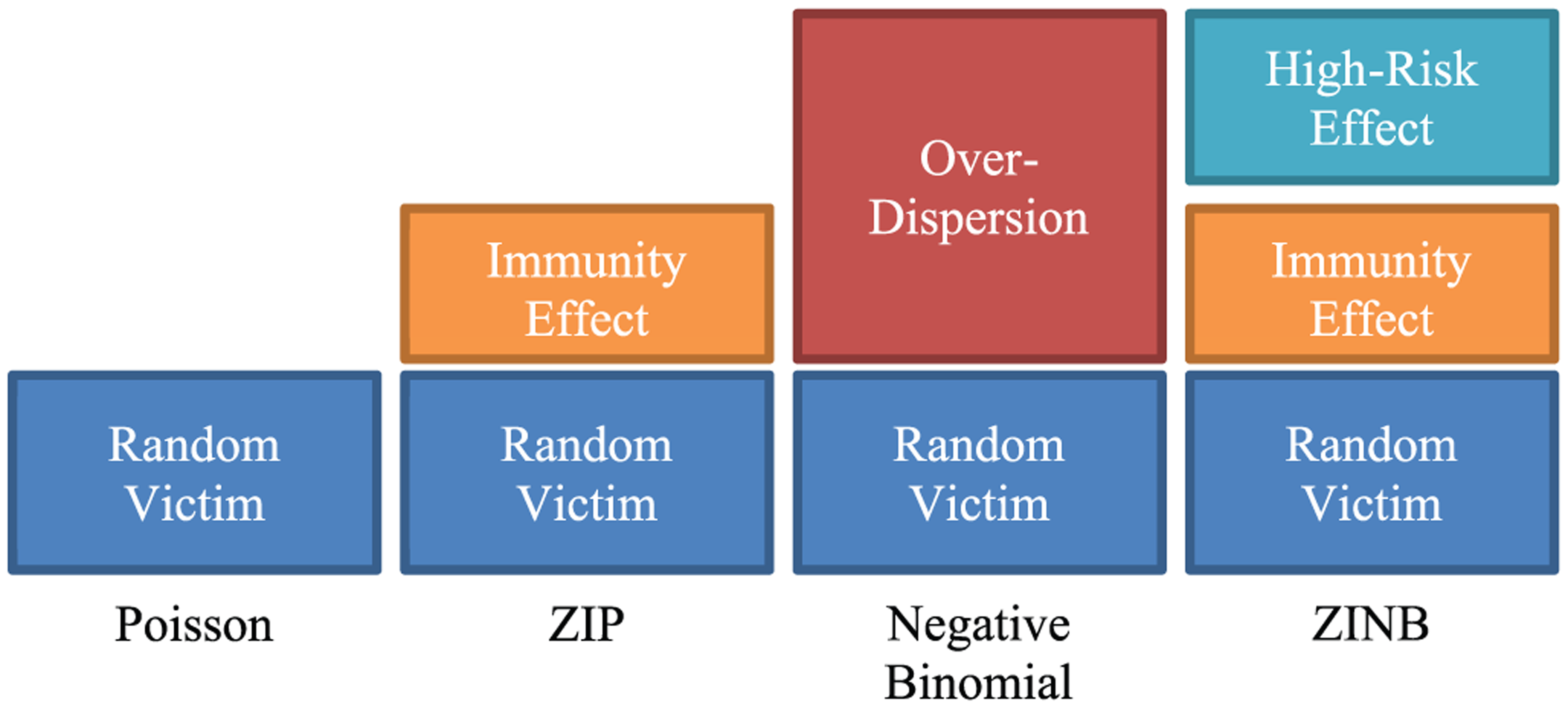
The negative binomial distribution, therefore, can be conceptually presented as two groups in the population: one group of targets who shares not-significantly-different risk of victimizations (random-risk group) and the other group of targets who are more victimization prone than those in the random-risk group (high-risk group). Following the Poisson distribution, the victimization frequency of the random-risk group is determined through the random and independent process, and some of them can be repeatedly victimized by chance 1 (random repeats, see Park & Eck, 2013). On the contrary, the victimization frequency of the high-risk group reflects their higher risk of victimizations, which is presented as the over-dispersion parameter in a negative binomial model.
Immunity and Zero-Inflated Models
Theoretical questions central to the immunity effect have been raised since the earliest studies on repeat victimization. In their study of the distribution of victimizations, Sparks et al. (1977) found that the observed distribution of victimizations did not fit the Poisson distribution and presented an “immune group” as a possible theoretical explanation for this lack of statistical fit. They defined an immune group as a portion of the population for whom the probability of becoming a victim is very close to zero, and argued that an immune group should be excluded from the study of victimization distributions to increase model fit (Sparks et al., 1977).
Years later, based on the model developed by Hope and Trickett (2004), Hope (2007) initiated a new perspective of immunity as a status of “negative exposure to crime risk.” He posited that there existed a nonrandom prevalence of immunity, and this nonrandom immunity was the reason for the difference in high crime areas in addition to high-risk repeat victimization (Hope, 2007). Extending Hope’s work, Hope and Norris (2013) presented two necessary factors to understand the heterogeneity in the distribution of victimizations: victimization frequency and victim prevalence. While nonvictims and high-level victims tend to retain their respective state, a general tendency and a tendency for low-level victims are toward nonvictimization (Hope & Trickett, 2008). They identified this general tendency toward nonvictimization as a complementary process of immunity, which is associated with victim prevalence (Hope & Norris, 2013). Analyzing the British Crime Survey and the Scotland Crime Survey data with the latent class analysis, they found that both victims’ propensities for immunity and exposure to crime victimizations are the interactive reasons of victimization distribution (Hope & Norris, 2013, p. 569).
Besides these theoretical and methodological developments in criminological studies, several statistical models were initiated to identify the effects of excessive zeroes in count data models (Winkelmann, 2008). To illustrate, Lambert (1992) initiated a new statistical model, the zero-inflated Poisson (ZIP), as a mixture of two independent processes: One generates only zero values, while the other generates numbers of incidents on the basis of the Poisson process. When applied to the distribution of victimizations, this model indicates that some immune targets (
The ZIP model also can be explained by the random chance of victimization. That is, introducing more zeroes to a victimization distribution artificially decreases its incidents rate. As the incident rate decreases, so does the expected random repeats (Park & Eck, 2013). Therefore, some of the random repeats in nonimmune targets (
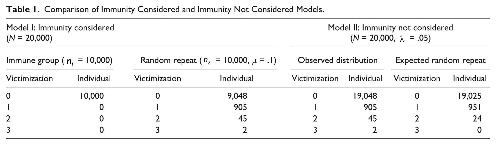
Comparison of Immunity Considered and Immunity Not Considered Models.
Statistically, the ZIP model rectifies this potential error by introducing two different equations: One is for the targets that have a zero probability of victimization and the other for the targets that have a nonzero probability, as follows:


where Y indicates the number of incidents (i.e., victimizations) and
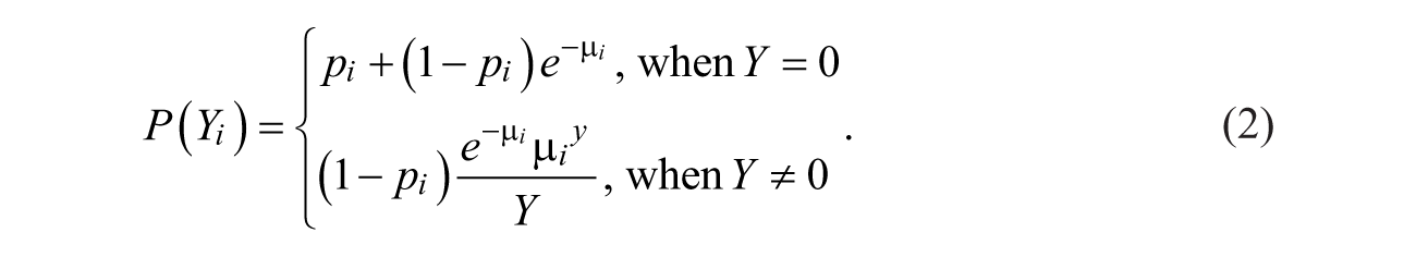
By introducing an immunity indicator parameter (

When the high-risk over-dispersion is anticipated over immunity, the zero-inflated negative binomial (ZINB) model provides a better fit to the victimization distributions. The ZINB model is an extension of this ZIP model (Winkelmann, 2008, p. 191). The probability function of the ZINB distribution can be obtained by applying a negative binomial to the ZIP distribution, which is presented as follows:


Here,
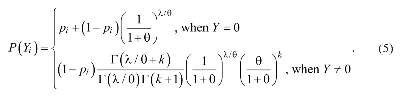
Again,
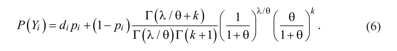
Hence, the ZINB II model is characterized as having both traits of the negative binomial and the ZIP models. The portion of the negative binomial shows the nonrandom effect of high-risk targets and event dependence. The ZIP part reflects both the zero-inflated effect from targets with extremely low risk and the random victimizations. In Equation 6,


One noticeable characteristic of the ZINB model is that introducing an immunity indicator (
Model-fit comparison among four count data models.
Considering the negative binomial model implies two groups in the population; the ZINB model can be conceptualized as three groups in the population: (a) a group of targets that have a zero probability to be victimized (immune group), (b) a group of targets that have a random chance to be victimized (random-risk group), and (c) a group of targets that have a higher probability to be victimized (high-risk group). While the second group members share random likelihood of victimizations, the third group members retain their own higher likelihood of victimization determined by their risk factors. This conceptualization is consistent with previous research. For example, Hope and Trickett (2008) showed that there were three levels of victims (nonvictims, low-level victims, and high-level victims) and found that each level of victims had a different probability for victimization.
Method
These statistical explanations of an immunity effect remain an open question whether the application of zero-inflated models does make a difference when testing the covariates of victimizations, and demand further empirical examinations. Analyzing a national-level victimization survey with both zero-inflated and non-zero-inflated models, this study investigates any difference that may arise from introducing a zero-inflated parameter to the analysis of victimization distributions.
Data
The data for this study are taken from the 2010 NCVS. Using a rotating panel sample design, the NCVS divided approximately 50,000 sample housing units into six rotation groups, and each group is interviewed every 6 months for a period of 3 years. For the interview process, six panels are designated in each rotation group, and a different panel is interviewed each month during a 6-month period. Each panel is interviewed seven times: The first and the fifth ones are face to face, and others are by telephone. After the seventh interview, the household is withdrawn from the panel, and a new household is introduced.
In 2010, a total of 66,268 households were interviewed for the NCVS. Among them, 40,703 households were surveyed twice, while the other 25,565 households had only one interview. As the number of random repeats is proportional to the length of time window (Park & Eck, 2013), only the households that completed two interviews are employed for this study, and the time window for a victimization to have occurred is 1 year. Out of the 40,703 households that completed two interviews, 13,854 households did not respond to the questions about previous household victimizations: Therefore, a total of 26,849 households are analyzed in the current study.
Dependent Variable
The number of the two types of victimizations experienced by households in 1 year is the dependent variable: burglary and auto theft. 2 Burglary victimization was operationalized using the following victimization screen questions: Has anyone (a) broken in or attempted to break into your home by forcing a door or window, pushing past someone, jimmying a lock, cutting a screen, or entering through an open door or window?; (b) illegally gotten in or tried to get into a garage, shed or storage room?; or (c) illegally gotten in or tried to get into a hotel or motel room or vacation home where you were staying? For auto-theft victimizations, the respondents were asked the following: Were any of your motor vehicles (a) stolen or used without permission?; (b) did anyone steal any parts such as a tire, tape deck, hubcap, or battery?; (c) did anyone steal gas from (it/them)?; or (d) did anyone attempt to steal any vehicle or parts attached to (it/them)?” If a respondent answered “yes” to any of the questions, the subsequent question asked the number of victimizations.
As observed in previous studies (Tseloni et al., 2004), the distribution of household victimizations is found to be highly skewed to the right. As shown in Table 2, while 25,947 households (96.6%) reported no victimization for both burglary and auto theft, 111 households (0.41%) were repeatedly victimized for 303 (27.7%) burglary or auto-theft crimes. More specifically, 46 (0.17%) households experienced 121 (29.2%) repeat burglary victimizations, and 54 households (0.2%) had 143 (21.0%) repeat auto-theft victimizations.
Frequency Distribution of Total Household Victimizations by Type of Crime.
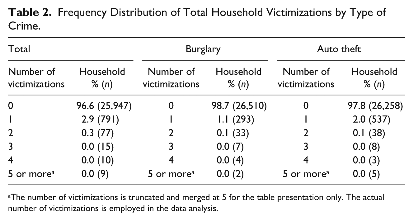
The number of victimizations is truncated and merged at 5 for the table presentation only. The actual number of victimizations is employed in the data analysis.
Explanatory Variable
The routine activity and lifestyle perspectives have addressed four risk factors for victimization: (a) target exposure, (b) guardianship, (c) attractiveness, and (d) proximity to motivated offenders (Cohen, Kleugal, & Land, 1981; Miethe & Meier, 1990; Tseloni et al., 2004). The present study includes these four risk factors as explanatory variables.
Target Exposure
Target exposure indicates an individual’s availability to be a victim (Meier & Miethe, 1993). For the study of household victimizations, target exposure has been conceptualized as physical visibility and accessibility of the residence (Bennett & Wright, 1984; Tseloni et al., 2004). The structural designs and types of dwellings determine the accessibility of the residence and also affect the risk of household victimization (Ellingworth, Farrell, & Pease, 1995; Osborn & Tseloni, 1998; Tseloni et al., 2004). For example, Miethe and Meier (1990) found that the dwellings detached from other units retained less visibility and, therefore, had higher risk of burglary.
The 2010 NCVS did not include a survey item that captured the degree of household physical visibility, which was the main aspect of target exposure in previous studies. Therefore, this study focused on the other element of target exposure, accessibility of the residence, and measured it with two variables: (a) type of living quarters and (b) operating a business. In the 2010 NCVS, respondents were given choices from typical residences such as house, apartment, and flat, to nontypical residences such as motel, mobile home, and rooming house. Compared with typical residences, nontypical residences are more accessible from outside and have been found to be more vulnerable to burglary (Ellingworth, Hope, Osborn, Trickett, & Pease, 1997; Osborn & Tseloni, 1998). The present study dichotomizes the type of living quarters into typical residence and nontypical residence; typical residence is the reference group. The second variable, operating a business, is operationalized by whether or not any of household members operate a business from the household’s address; not operating a business from the residence is the reference group.
Guardianship
Guardianship refers to the capability of persons and objects to prevent crimes from occurring (Tseloni et al., 2004). Studies on household victimization generally classified guardianship into social and physical guardianships (Garofalo & Clark, 1992; Meier & Miethe, 1993; Tseloni et al., 2004).
Social guardianship
Social guardianship indicates availability of others who may prevent personal crimes by their mere presence or by offering assistance to ward off an attack (Miethe & Meier, 1990). Past research has operationalized social guardianship measures with household composition, house occupancy, and existence of neighbors watching unoccupied house in the community (Tseloni et al., 2004). Social guardianship measures also have been used as a proxy lifestyle indicator of household, because it reflects the extent to which the residence is left unoccupied (Tseloni et al., 2004). Studies consistently reported that the amount of emptiness and the number of adults significantly affected the odds of burglary victimizations (Bennett & Wright, 1984; Ellingworth et al., 1997; Hough, 1984; Miethe, Stafford, & Long, 1987; Osborn & Tseloni, 1998; Tseloni et al., 2004).
Building from these findings, three variables were used to capture social guardianship: (a) family structure, (b) household composition, and (c) multiple housing units. Family structure is measured by whether the household is a lone parent family. Tseloni et al. (2004) reported a positive relationship between lone parent households and the chance to be burglarized. Household composition is operationalized as the total number of residents who are 12 or older. The last variable of “multiple housing units” distinguishes whether there is single housing unit or two or more housing units in the dwelling; single housing unit is the reference group.
Physical guardianship
Physical guardianship indicates the use of self-protection measures and participation in collective crime prevention activities (Meier & Miethe, 1993; Tseloni et al., 2004). While some studies found that physical guardianship significantly decreased the risk of household victimization (Budd, 1999; Miethe & Meier, 1990; Miethe & McDowall, 1993), others found that higher physical guardianship was combined with higher odds of household victimization (Tseloni & Farrell, 2002; Tseloni et al., 2004). Tseloni et al. (2004) explained this discrepancy as a result of inconsistent temporal order between victimization experience and initiation of guardianship. In the present study, two survey items are used to measure physical guardianship: whether or not gated or walled community and whether or not building with restricted access. The variable of physical guardianship is operationalized as the total number of “yes” responses to these two questions and ranges from zero to two.
Target attractiveness
Target attractiveness indicates the availability of properties with high economic or symbolic values (Meier & Miethe, 1993; Miethe & Meier, 1990; Tseloni et al., 2004). Motivated offenders were assumed to pursue more economic gains by targeting geographical locations or households with better exterior condition (Cromwell, Olson, & D’Aunn Wester, 1991; Meier & Miethe, 1993). As a result, households with higher income or education had higher odds of household victimization, as they are expected to have more valuable goods (Cohen et al., 1981; Miethe & Meier, 1990). Previous studies have used household income and level of education as the measures of target attractiveness (Tseloni et al., 2004). The present study also operationalizes target attractiveness with household income, education level of a principal respondent, and ownership. Household income was measured with 12 categories from “less than US$5,000” to “US$75,000 or higher.” Education level was measured with 27 categories from “none” to “doctoral grade.” Ownership of residence is operationalized as a dichotomous variable indicating whether or not the respondent owns or rents a house; home ownership is the reference group.
Proximity to potential offenders
Proximity to potential offenders refers to the physical distance between potential targets and motivated offenders (Meier & Miethe, 1993; Tseloni et al., 2004). It has been argued that living in a high crime or disorder area increases the odds of victimization (Miethe & Meier, 1990; Tseloni et al., 2004). For example, residents in areas with higher levels of offenders, inner city, low-income area, or council houses were found to suffer from higher odds of household victimizations (Cohen et al., 1981; Ellingworth et al., 1997; Miethe & Meier, 1990; Osborn & Tseloni, 1998; Tseloni et al., 2004). Previous studies also revealed the commercial places are more frequently victimized (Shury, Speed, & Vivian, 2005). In the present study, proximity to potential offenders is measured with whether a respondent resides in a rural or urban area; residing in an urban area is the reference group.
Control variables
In addition to four risk factors, the demographic characteristics of the reference respondent in each household, such as age, gender, and race, were included in the model as control variables. Age is measured with the actual age of a reference person in years. The distribution of age was from 12 to 90 years. Race of the reference respondent is either a White or non-White; White is the reference group. Table 3 presents the descriptive statistics for all the variables. The variance inflation factor (VIF) values for bivariate combinations of explanatory variables ranged from 1.005 to 1.945 indicating little multicollinearity among variables.
Descriptive Statistics of Variables (N = 26,849).

Analysis
To select an optimum statistical model, the goodness-of-fit of four count data models are tested. Previously, the
Two types of information criterion (IC) are employed to test the goodness-of-fit of four count data models: the Akaike Information Criterion (AIC) and the Bayesian Information Criterion (BIC). The general form of IC is given as:

where
Table 4 provides the model-fit statistics of four intercept-only count models. The model-fit test of the full model, which is obtained by data-driven model selection, is not employed in the current study, as recent studies have revealed that data-driven model selection yields biased estimation of
AIC and BIC Model-Fit Test for Intercept-Only Models.
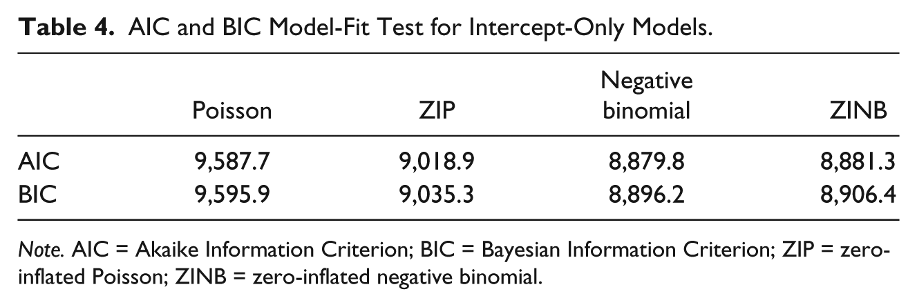
Note. AIC = Akaike Information Criterion; BIC = Bayesian Information Criterion; ZIP = zero-inflated Poisson; ZINB = zero-inflated negative binomial.
As presented in Figure 1, the better model fit of the ZIP over the Poisson shows that there exists an immunity effect indicating that a group of households have zero probability to experience a household victimization. The better model fit of the negative binomial over the ZIP represents that there are remaining over-dispersed victimizations that cannot be explained only by immunity effect. As explained in the previous section, the ZINB, however, does not show better model fit over the negative binomial. Adding the immunity parameter to the negative binomial model, on the contrary, reduces model fit in both AIC and BIC statistics because the number of parameters in the Equation 9 (
Zero-Inflated Regression
To capture the influence of covariates on the inflation of zeroes, Lambert (1992) initiated the ZIP regression and specified the probability of extra zeroes as a logit model

Here,

Hence, the covariates of Poisson regression part (
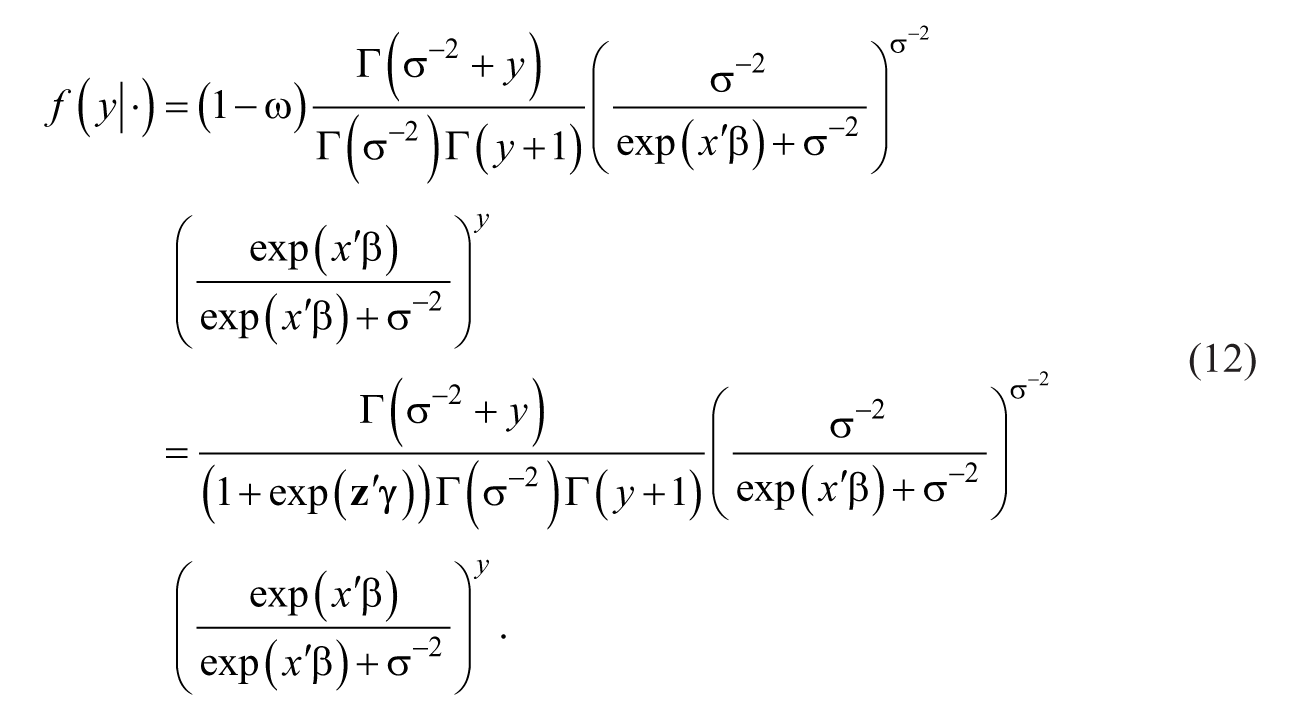
As shown in Equation 12, the ZINB regression also retains two sets of covariates. The negative binomial coefficients (
Control for Multiple Testing—Benjamini and Hochberg Method
When multiple hypotheses are tested in a statistical analysis, the amount of Type I error increases as the number of hypotheses increases. If a significance level (
The widely used procedure for controlling for Multiple Testing is the Bonferroni method, where a new

While the Benjamini and Hochberg method proved to be a powerful tool and better than other controlling methods or tests without the adjustment (see Pawluk-Kolc, Zieba-Palus, & Parczewski, 2006), the application of this method is not common in criminal justice studies (i.e., Lane, 2009). The present study employs the Benjamini and Hochberg method to inform the decision about significance when controlling for Multiple Testing.
Findings
The results from both the negative binomial regression and the ZINB regression are presented in Table 5. A total of 9 out of 13 explanatory variables show the consistent findings across both models. After considering the immunity effect, however, the other four variables are found to possess different effects on the risk of household victimization. Even for the variables showing consistent influence in both models, the ZINB regression identifies additional effects and/or different expected changes. Overall, the target attractiveness, physical guardianship, and proximity to offender variables have consistent effects in two models. On the contrary, the target exposure, social guardianship, and demographic measures influence household victimization differently between two models.
Comparison Between Negative Binomial and Zero-Inflated Negative Binomial Regressions.

Note. Vuong test of ZINB over negative binomial: z = 2.65** (p = .004). ZINB = Zero-inflated negative binomial.
Statistically significant after Benjamini and Hochberg Correction at *
For target attractiveness, only the ZINB regression reveals a significant effect that those who dwell in nontypical residency are found to have significant higher odds of experiencing a household victimization. This finding is consistent with previous studies, which found that detached or semidetached houses were more vulnerable to household victimizations (Ellingworth et al., 1997; Osborn & Tseloni, 1998; Tseloni et al., 2004). In addition to this finding, the ZINB model reveals that target attractiveness does not significantly influence the probability of being immune to household victimization. That is, while residents living in typical residences have significantly lower probabilities to be victimized, they still have the same odds to be immune and are exposed to random victimizations.
The negative binomial and the ZINB models also present different findings for one of three social guardianship variables: lone parent family. The negative binomial regression finds that lone parent families do not have significantly different odds to be victimized from those with both parents. The ZINB, however, finds that families with both parents have significant higher chance to possess immunity. On the contrary, the effect of lone parent family on high-risk estimation in the ZINB shows that families with both parents do not retain significantly different odds of victimization from lone parent families after excluding the immune group from the analysis. For other social guardianship variables, household composition and multiple housing, both the negative binomial and the ZINB regressions fail to find any significant impact on household victimization.
In the analysis of physical guardianship variable, the ZINB model presents nonsignificant, but noteworthy, polarizing effect. Previous studies have revealed inconsistent influence of physical guardianship. In the present study, the ZINB shows that more physical guardianship is connected to lower risk of victimization as found in the negative binomial regression. In addition, it finds that higher level of guardianship is associated with less probability to be immune. Despite the lack of statistical significance, this polarizing directionality may provide a possible explanation of the previous contradictory findings. That is, households may reduce the risk of victimization by initiating more physical guardianship; on the contrary, the more physical guardianship indicates the less immunity to the risk of victimization.
The effects of target attractiveness and proximity to offenders variables are found to be consistent between the negative binomial and the ZINB models. Both models find that lower income, residing in rented units, and living in an urban area are linked to significantly higher chance of victimization. One noticeable difference between two regressions is that the ZINB analysis consistently reveals that the effects of those variables are stronger than expected by the negative binomial analysis. For example, the coefficient in the negative binomial regression estimates the expected change of the mean victimization count to be 1.57 (
The findings from the analysis of two demographic variables—age and race—are also contradictory and inconsistent between the negative binomial and ZINB models. Contrary to the significant negative effect of age on the high risk of victimization in the negative binomial regression, the ZINB presents only the significant positive effect of age on immunity: When the respondent is getting older, only the odds to be immune significantly increase, but the high risk of victimization does not significantly change. For the effect of race, the negative binomial regression finds significantly higher odds of victimization for non-White: However, the ZINB reveals that there is no significant difference between White and non-White households.
Discussion
By reviewing the zero-inflated statistical models and comparing the results from zero-inflated and non-zero-inflated models, the present study aimed to empirically test the effect of immunity on the distribution of household victimizations from the 2010 NCVS. For the analysis of aggregate-level frequency distributions in a given period, the ZINB model conceptually postulates that there subsist three groups of individuals in the population: (1) the immune group which has extremely low probability to be victimized; (2) the random-risk group, which shares homogeneous and independent chances of victimizations; and (3) the high-risk group, which retains higher propensity to be victimized. To identify the determinants of both immunity and high risk, the ZINB model separates the population into the immune group and nonimmune group, and introduces two sets of coefficients accounting for the probability of zero inflation and the odds of higher household victimization counts.
The results have presented that the existence of an immune group necessitates the application of the zero-inflated models. By reducing the expected count of random repeats, immunity contributes to the increase of over-dispersion in the victimization distribution. As shown in the simulation of Table 2, failure to consider the effect of immunity leads to the erroneous identification of random repeats as high-risk victimizations. Furthermore, the comparison of the ZINB and the negative binomial models revealed that this failure might result in inconsistent interpretations of covariates. As discussed below, the ZINB model identified more diverse aspects of covariates, which were not distinct in the negative binomial model.
Despite of the benefits from the zero-inflated models, it is not clearly intuitive to identify the existence of an immune group in the population. The intercept-only ZINB model does not provide a better model fit over the negative binomial model, even when there exists an immune group. The model-fit comparison of the full models with insignificant covariates should be used with caution, as these covariates also influence the amount of model fit by chance. Furthermore, recent studies have identified that the data-driven model selection yields biased estimation of coefficients (Berk et al., 2013; Berk et al., 2010; Leeb & Po ̈tscher, 2005, 2006; Lockhart et al., 2014). To address this issue, the present study proposed a model-fit comparison of four intercept-only count models: the Poisson, the ZIP, the negative binomial, and the ZINB. As described in Figure 1, the better model fit of the ZIP over the Poisson represents the effect of the zero-inflated parameter, while that of the negative binomial over the ZIP indicates the remaining over-dispersion after fitting zero-inflation and random processes.
Compared with that of the negative binomial model, two sets of coefficients in the ZINB model revealed more complex and dynamic influence of the covariates in this study. For instance, while the negative binomial regression failed to find any significant effect of lone parent family, the ZINB regression identified its significant negative effect on immunity. The significant higher odds of victimization for non-White in the negative binomial model dissipated when the immunity effect is introduced in the ZINB model. In the case of age, while older residents were found to have a lower chance of victimization in the negative binomial model, the ZINB model showed that the older respondents have higher odds of immunity.
As shown in the case of physical guardianship, one noteworthy finding from the ZINB regression was the polarizing effects of some variables. The polarizing effect is defined here as the same directional effects on both immunity and high risk are identified from one variable. For example, the insignificant coefficients of physical guardianship can be interpreted as the households with more physical guardianship retain lower odds of household victimization: However, they also have a lower chance to be immune. Considering that the ZINB regression separates the population into immune and nonimmune groups with zero-inflation covariates, and then identifies covariates for higher risk of victimization, this polarizing effect can imply that households with more physical guardianship are less likely to be immune to household victimizations. After excluding an immune group from the analysis, however, the remaining households with more physical guardianship retain a lower chance to be victimized than those with less physical guardianship.
Finally, the limitations of this study should be addressed for the further clarification of immunity effect. First, random repeats and/or immunity effect are not necessarily embedded in all types of victimization distributions. For some types of victimizations that are based on a specific relationship between the offender and victim, such as domestic violence, it is more reasonable to assume that there is no random repeat. If there is no chance that offenders randomly select victims, the immunity effect does not influence the estimation of high-risk victimization. This conditional aspect indicates that the victimization distribution is also determined by the relationship between offenders and victims, not solely by victims’ risk (e.g., lifestyle or routine activity).
Second, the hurdle model also is frequently employed to address excessive zeros in other fields and study (see Winkelmann, 2008, for specific examples). The main difference between the hurdle model and the zero-inflated model is that the former artificially separates
Third, there are limitations that originated from the NCVS data. As this study used the NCVS as a cross-sectional format, the effects of event dependence and/or risk heterogeneity on the victimization distribution were not examined. Furthermore, the present study did not take into account possible selection bias from missing cases who did not report household victimizations. Random measurement errors also may have been introduced as explanatory variables were measured as proxies.
Fourth, the present study is primarily concerned with the methodological issues for the analysis of immunity effect, and does not focus on the theoretical and policy implications of immunity. To fully understand the diverse victimization statuses in the population, the causality of immunity should be theorized, scrutinized, and integrated into the empirical analyses of predicting victimization. Previously, for example, ethnographic studies on offenders were mainly concerned about how and why they chose targets (i.e., Clare, 2009). The immunity effect argument, however, suggests that the information on why offenders did not choose a certain type of targets is also important to increase the effectiveness of crime prevention efforts. In addition, as discussed, the various relationships between offenders and victims should be integrated into understanding victimization distributions. These findings imply that crime prevention efforts targeting only previous repeat victims may not fully address the totality why targets are victimized. To effectively prevent crimes by reducing future victimizations, policy makers should also take into account other factors including immunity, random repeats, and offender-victim relationships. A next logical step for future studies focused on victimization distributions, therefore, is the clarification of the existence or nonexistence of an immune group and/or random repeats for other types of victimizations.
Conclusion
The findings of this study provide additional support to the recently initiated argument that over-dispersed distribution of criminal victimizations is the result of more complex and diverse population statuses than previously expected. In addition to risk heterogeneity and event dependence, random repeats and immunity effect also can influence the frequency distribution of victimizations. When there exists a group of targets characterized by an extremely low probability of victimization in the population, a failure to consider the immunity effect may result in incorrect identification of high-risk targets and wrongful estimation of over-dispersion predictors. The results of this study, therefore, suggest that future studies analyzing repeat victimization distributions should test the existence of an immune group, use both zero-inflated and non-zero-inflated models, and compare the results to determine whether there are different findings between these models. Future studies will be able to better clarify the dynamics underlying repeat victimization processes by incorporating different theoretical approaches, exploring more diverse determinants, and analyzing different types of criminal victimizations.
Footnotes
Declaration of Conflicting Interests
The author(s) declared no potential conflicts of interest with respect to the research, authorship, and/or publication of this article.
Funding
The author(s) received no financial support for the research, authorship, and/or publication of this article.