Spatial Modeling in Neighborhood and Crime Studies: An Empirical Examination

Abstract

We theoretically discuss why addressing spatial dependence is important and empirically demonstrate its methodological advantages in the context of neighborhood and crime studies. We found that as the uncertainty in measuring neighbors increases, the bias in the coefficient estimates increases. However, importantly, we also observed that even with a high rate of uncertainty in the spatial matrix, the bias is smaller than in the non-spatial models. Likewise, as the uncertainty in defining neighbors increases, models tend to underestimate the standard errors. However, even with higher uncertainty in the spatial weight matrix, underestimation seems smaller than that of the non-spatial model.

Keywords

spatial analysis neighborhoods crime

Introduction

Over the last few decades, a substantial body of ecological studies on crime has found that certain places or neighborhoods within a city exhibit higher levels of crime than others (Weisburd, 2015; Weisburd et al., 2012). Many studies examining neighborhoods and crime have empirically revealed that spatial crime concentration stems from specific structural characteristics inherent to neighborhoods (Hipp, 2007; Sampson, 2012; Sampson et al., 1997). For example, studies focusing on social structural characteristics often draw from social disorganization theory as their theoretical basis. The theory posits that certain structural features of a neighborhood, such as socioeconomic disadvantage, racial composition, residential mobility, or racial heterogeneity undermine social ties and cohesion. Consequently, this leads to a reduced level of informal social control and collective efficacy among residents, thereby increasing crime rates.

While the primary focus has been on the association between measures of structural characteristics and crime within a focal neighborhood, some studies have also provided theoretical justifications and empirical evidence for the importance of incorporating “neighboring” areas. Theoretically, this is because a neighborhood is not a physical or social island but rather interconnected with adjacent and nearby areas in terms of social and environmental development and change. Moreover, residents define and perceive their neighborhoods more expansively than predefined spatial boundaries, and their mobility patterns extend beyond a specific area of residence, which has significant implications for spatial crime patterns.

Indeed, previous research has extensively focused on structural characteristics and neighborhood crime while recognizing and integrating the significance of nearby areas, thereby acknowledging the spatial interdependencies of crime and its determinants. This has been accomplished by utilizing various methodological tools of spatial regression modeling (Browning et al., 2004; Morenoff et al., 2001). While some studies have incorporated spatial lagged terms of crime on the right-hand side of a regression equation, others have attempted to address spatial dependency by including a set of spatially lagged independent variables (or both), or spatial error term, etc.

Putting aside which modeling strategy is more accurate or suitable for a neighborhood and crime study—an issue that should be guided by plausible theoretical specification and justification (e.g., see Cook et al., 2023; Griffth, 1996)—we need to examine whether considering the spatial effects of nearby areas is theoretically and methodologically preferred. In other words, to what extent accounting for spatial dependency in a neighborhood and crime study may bring about empirical advantages, which is a question previous studies have paid less attention to. In the current study, we aim to provide empirical evidence of whether addressing spatial dependence dominates non-spatial models in the context of a neighborhood and crime study.

Another important methodological consideration in employing spatial models concerns the uncertainty surrounding the specification of spatial proximity—that is, how “nearby” or “neighboring” units are defined. For doing so, the choice of spatial weight matrix plays a critical role in determining the degree and structure of spatial dependence captured by the model. Different conceptualizations of neighborhood associations (e.g., contiguity-based vs. distance-based weights) can yield varying estimates and interpretations of spatial effects. Therefore, it is necessary to empirically assess whether spatial modeling strategies truly provide empirical advantages, even in the presence of uncertainty in defining what constitutes “nearby” and in addressing spatial dependence among the spatial units—a topic that has received limited attention in prior research. Specifically, this study seeks to address two closely related questions: (1) Do spatial modeling strategies offer empirical advantages over non-spatial models for understanding neighborhood and crime relationships? and (2) If so, are these advantages robust to uncertainty in the definition of “nearby” areas when modeling spatial dependence?

Note upfront to clarify that the primary motivation for the current study is not necessarily arguing that previous studies of neighborhood and crime have not accurately accounted for the spatial dependency, nor have they failed to address such methodological issues. As discussed in-depth in the following sections, we recognize the important theoretical insights and methodological advancements provided by prior research. Then, building upon prior work, the current study aims to contribute to the field by enhancing the theoretical and methodological discussion on spatial modeling strategies as well as providing empirical evidence that reinforces the importance of incorporating spatial dependency when studying neighborhoods and crime. In the subsequent sections, we discuss our theoretical and methodological motivations corresponding to the two research questions posed above, along with our empirical approaches.

Research Background

A large body of neighborhood and crime studies has confirmed that crime is not randomly distributed over space but rather spatially clustered in certain neighborhoods in any geographical unit. Similarly, prior research has suggested that certain structural characteristics of neighborhoods are associated with reduced or increased levels of neighborhood crime. Social disorganization theory underpins many of these studies. The theory contends that certain structural characteristics (e.g., socioeconomic disadvantage, residential turnover, or racial heterogeneity) may disrupt the process of building social ties and cohesion among residents, which in turn leads to a reduced level of informal capability to address the local neighborhood problems (including crime and disorder) by residents themselves.

While the theory primarily focuses on how the structural characteristics of a specific neighborhood are crucial for explaining crime within that locality, related studies have also acknowledged the significance of considering structural characteristics in nearby areas and even within a broader regional context (Hipp & Roussell, 2013; Hipp et al., 2017; Peterson & Krivo, 2010). This broader perspective has received scholarly attention because neighborhoods are not isolated from their surrounding areas (Anselin, 1988, 2002; Baller et al. 2001; Mears & Bhati, 2006). Specifically, the structural characteristics of neighborhoods do not develop exclusively within the confines of each neighborhood; instead, they have a broader impact that extends beyond specific neighborhood boundaries. For instance, socioeconomic disadvantage in a particular neighborhood not only affects that neighborhood but also influences other nearby areas, shaping crime patterns in the broader region. Thus, the attributes of crime or structural characteristics in surrounding areas can have an impact on crime in a particular neighborhood, regardless of the boundaries used to define and measure the neighborhood. Therefore, it is more reasonable to incorporate nearby areas when defining neighborhoods, measuring their structural characteristics, and examining their associations with crime (Boessen & Hipp 2015; Hipp & Kubrin, 2017; Peterson & Krivo, 2010).

Furthermore, neighborhood residents do not necessarily perceive their neighborhood boundaries as physically or psychologically confined to a specific area. Instead, they tend to consider some amount of nearby areas surrounding their focal residential areas when defining and conceptualizing their neighborhood boundaries. Likewise, residents’ perceptions of social surroundings spatially extend beyond the pre-defined focal neighborhood boundary (Boyd & Richerson, 1985; Hunter, 1974; Janowitz, 1952; Lynch & Addington, 2006). Moreover, since residents’ perceptions of their neighborhood spatially transcend their immediate residential areas, residents’ mobility (Lee & Kwan, 2011; Ren & Kwan, 2009) and routine activity patterns (Felson & Boba, 2010) may also extend beyond specific spatial boundaries. Consequently, disregarding neighboring areas may overlook important implications for defining neighborhoods and, as a result, understating neighborhood crime.

Accounting for Spatial Dependency in Neighborhood and Crime Study

In a conventional regression practice (not in a spatial context), researchers tend to assume no unit dependency when estimating the effects of primary explanatory variables on a dependent variable. This holds true for both ordinary least squares and maximum likelihood estimation, applicable to continuous and categorical dependent variables. This assumes that changes in the explanatory variables within a specific unit are associated with corresponding changes in the dependent variable within that unit only. However, if the explanatory variables (or the dependent itself) affect the dependent variable in other units indicating the presence of spillover effect, we cannot be certain of the isolated impact within the intended unit. This is particularly relevant in neighborhood and crime studies as abovementioned. Therefore, for a neighborhood and crime study, it is essential to address the spatial dependencies among the variables included in models to maintain the integrity of the model assumptions, foster confidence in the validity of the parameter estimates, and support robust statistical analysis.

Although there are many different modeling strategies to address spatial dependence, two methodological approaches have been widely employed in previous studies of neighborhoods and crime to understand how surrounding areas impact crime. The two are based on the following assumptions that: (1) Crime in nearby areas influences the level of crime in a given focal neighborhood directly; and/or (2) Certain structural characteristics in nearby areas (in)directly influence the level of crime in a given focal neighborhood. The first approach (e.g., a model with a spatial lagged dependent variable of crime outcome or so-called “Spatial Lag Model—SLM”) assumes an endogenous interaction between crime in a focal neighborhood and its nearby areas in which the crime outcome in the focal unit depends on crime outcomes in surrounding areas as defined in the spatial weight matrix (W). The spatial weight matrix functions like a map that illustrates the closeness or connectivity between various locations. It assigns values to pairs of locations according to their proximity or relationship by definition. For example, closer locations may receive a high value in the matrix, indicating a stronger association. The SLM accounts for spatial autocorrelation and the underlying spatial structure within the data by incorporating the spatial weight matrix into estimation. Therefore, it presumes a spatial contagion or diffusion effect of crime, treating the risk of crime as a contagious disease where crime in one area may directly increase or decrease crime in other adjacent areas (Cohen & Tita, 1999; Loftin, 1986; Messner et al., 1999; Papachristos et al., 2015).

For such a modeling strategy, it is crucial to be guided by plausible theoretical justifications how and why crime in one area can be directly contagious to neighboring areas without requiring additional theoretical mechanisms to explain how the spatial qualities (i.e., structural characteristics or the opportunity structure) in surrounding areas may indirectly impact crime in a given focal neighborhood. For instance, in a study of homicide in Chicago neighborhoods, Morenoff et al. (2001) have employed such an approach based on a theoretical motivation that “. . . interpersonal crimes such as homicide are based on social interaction and thus subject to diffusion processes . . . Thus, a homicide in one neighborhood may provide the spark that eventually leads to a retaliatory killing in a nearby neighborhood” (p. 523). Browning et al. (2004) adapted this theoretical perspective of the “spatial vulnerability” of homicide and employed a similar modeling strategy.

Nonetheless, in crime and place or neighborhood and crime literature, theoretical mechanisms often focus more on nearby structural characteristics and the expected spatial influence of them on crime level in a given focal neighborhood (Bernasco & Block, 2011; Haberman & Ratcliffe, 2015; Hipp & Kubrin, 2017; Wo et al., 2016). This is because it is theoretically more plausible to pose (or safer to assume) that environmental features in nearby areas influence the risk of crime in a given focal neighborhood rather than simply assuming that crime spatially spreads like a contagious disease, unless a reasonable theoretical justification is provided. Therefore, as long as the risk of crime is determined by the ecological structural characteristics of a neighborhood (i.e., concentrated disadvantage, racial diversity, or the level of informal social or collective efficacy), “spatial proximity to such conditions is also likely to influence the risk of crime in a focal neighborhood” (Morenoff et al., 2001, p. 522). This is because, as discussed above, neighborhood structural characteristics tend to develop and change on a broader spatial scale larger than a pre-defined neighborhood boundary commonly employed (e.g., Census blocks, block groups, or tracts). Therefore, certain types of structural characteristics of a particular geographical unit are likely to be associated with crime in that unit but also in nearby areas.

Methodologically speaking, in this case, spatial spillover effects in the independent variable are likely, which may violate the assumption in the linear regression and causal inference context that an independent variable concerning one unit impacts the dependent variable in that unit exclusively. To address this, researchers frequently employ a Spatially Lagged X Model—SLX with a spatially lagged independent variable. Such a model can be generally expressed as $y_{i} = α + X_{i β} + W X_{i} θ + ε_{i}$ where captures the effect of spatial qualities (e.g., structural characteristics) in neighboring areas on crime in a given focal neighborhood. Therefore, if spillover effects of independent variables are theoretically and empirically expected, the SLX model is methodologically preferred as employing a common regression model in such cases may introduce bias and inefficiency to the estimates. In the subsequent section, we provide a detailed methodological discussion on this bias and inefficiency.

Ignoring the Spatial Dependency: Bias and Uncertainty

Given the theoretical motivations discussed above for considering nearby areas, in this section, we provide methodological considerations about a hypothetical model that fails to properly account for the spatial influence of surrounding areas. We employ SLX chosen for theoretical and illustrative convenience.¹ However, other models can also be applied including the one assuming spatial dependencies in the dependent variables as well as the error terms, based on the spatial theory of interest and the available data. Further information can be found in works by others (Anselin et al., 2000; Betz et al., 2021; Cook et al., 2023; LeSage & Pace, 2009). We also provide detailed derivations in Supplemental Appendix B. First, let’s consider the true data-generating process as follows when we anticipate the existence of spatial dependencies in the determinants (X) affecting crime (Y):

y_{i} = α + X_{i} β + W X_{i} θ + ε_{i}

(1)

where $y_{i}$ is a dependent variable, $X_{i}$ is the matrix of independent variables, β is for the vector of coefficients, W represents the matrix of spatial lagged measures, θ is for the vector of spillover effects, α is for the intercept, and $ε_{i}$ is an error term. However, we assume a situation where we run a model that does not take spatial dependency into account resulting in the following estimated model. Here, $e_{i}$ is the error term in the model that does not account for the spatial dependence:

{\overset{\land}{y}}_{i} = α + X_{i} \overset{\land}{β} + e_{i}

(2)

Now, let X be the matrix of independent variables, y be the vector of the dependent variable, and e be the vector of residuals. Then, the estimate $\overset{\land}{β}$ can be written as if no spatial dependencies exist:

\overset{\land}{β} = {(X' X)}^{- 1} X' y

(3)

Then, the expected value of $\overset{\land}{β}$ can be expressed as:

E (\overset{\land}{β}) = β + \frac{c o v (X, W X θ)}{v a r (X)}

(4)

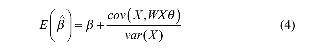
Therefore, the expected value of $\overset{\land}{β}$ when omitting the spatially lagged independent variable term is given by the true β plus $\frac{c o v (X, W X θ)}{v a r (X)}$ . If there is no assumed spatial dependence in X, then the $c o v (X, W X θ) = 0$ , so $E (\overset{\land}{β}) = β$ , which indicates there is no bias in the estimator. However, if spatial dependence exists, which is more theoretically plausible in the neighborhood and crime study, in particular, even with a small degree, $\frac{c o v (X, W X θ)}{v a r (X)}$ is not equal to zero, thus the estimator will have bias.

Moreover, the neglect of accounting for the spatial dependence can lead to underestimation of the uncertainty of parameter estimates. This arises from the failure to account for the spatial dependence captured by the spatial lag term in X, leading to an overestimation of the precision of the estimated coefficients. Consequently, hypothesis tests may be overly confident, leading to potential Type I errors (false positives) and unreliable conclusions about the significance of coefficients. To understand this, let us consider the expected value of $\overset{\land}{β}$ . If we neglect the spatial lag term in the calculation of $S E (\overset{\land}{β})$ , we end up with:

v a r (\overset{\land}{β}) \approx σ^{2} {(X' X)}^{- 1}

(5)

This approximation ignores the additional spatial dependence term, leading to inefficient standard errors. As a result, hypothesis tests and confidence intervals based on these standard errors may lack precision and reliability.² In summary, neglecting the spatial dependence in the model estimation not only introduces bias but also results in the underestimation of the precision of our estimators.

Uncertainty When Defining “Nearby”

Another critical issue when employing spatial modeling strategies in neighborhood and crime studies is about the definition of nearby. To be realistic, what constitutes nearby areas can be largely contingent on how a researcher defines and specifies the optimal spatial weight matrix, which ostensibly varies across research contexts and theoretical motivations. For instance, one might define neighbors of a given area based on the spatial contiguity of a given spatial boundary to other surrounding areas (Bernasco & Block, 2011; Browning et al., 2004; Morenoff et al., 2001; Sampson et al., 1997). Such a way defines neighbors as immediate surrounding areas that geographically share the physical boundaries with a given focal neighborhood based on spatial adjacency. However, a critical uncertainty regards to what spatial extent one should consider neighbors of a given focal neighborhood (e.g., the first or second order, rook, bishop, or queen contiguity); how to define a shared boundary; or how many of them should be considered as neighbors (e.g., K-nearest neighbors).

Others have turned to a distance-based approach when defining neighbors of a given neighborhood. The underlying assumption is that nearby areas matter but those closer in proximity matter more—the distance decay effect. Particularly, in a neighborhood and crime study context, the distance decay function provides important implications. Specifically, the formation of social ties follows the distance decay function as residents are more likely to socially interact and build social ties and trust with other residents living closer to their own home than to those farther away. Therefore, individuals are more likely to form social networks and ties with those who are in closer proximity in physical distance so that they can minimize the effort and cost. This has been consistently observed in previous studies that the physical distance with a distance decay effect is a strong factor in determining social networks and ties among residents (Rick, 2009; Hipp & Perrin, 2009; Mayhew & Levinger, 1976). Given that the formation of social ties, building social cohesion among residents, and further development of informal social control and collective efficacy are at the core of social disorganization theory for explaining neighborhood crime, incorporating the distance decay aspect when defining neighbors of a given neighborhood seems theoretically plausible.

However, an uncertainty regarding the definition of neighbors based on the distance decay function lies in the radius distance itself. That is, it is methodologically arbitrary how far distance a researcher should consider when defining nearby areas. One common methodological approach is to create spatially lagged measures based on an inverse distance function with a cutoff at a specific distance around a focal unit. Those beyond the distance cutoff will have a value of zero in the spatial weight matrix, W. Then the resulting spatial weights matrix is row standardized and is multiplied by the matrix of values in the focal neighborhood for the variables of interest. However, by nature, this approach requires an arbitrary and abrupt breakpoint at a certain distance (e.g., 1/4, 1/2, 1 mile, etc.) and areas within the defined distance from the focal area will be considered as neighbors while those beyond that distance will be treated having completely no spatial effect on the focal area. Although prior work commonly employed a 1/4- or 1/2-mile distance cutoff (Boessen & Hipp, 2015; Kim & Hipp, 2020; Rengert et al., 1999), it is largely uncertain what constitutes the optimal distance radius for defining neighbors based on distance decay, which arguably varies by research contexts and theoretical motivations and justifications.

In sum, we have outlined the theoretical and methodological advantages of employing spatial modeling strategies within the context of neighborhood and crime research. Building upon these foundations, our analysis seeks to demonstrate the empirical benefits of spatial models relative to their non-spatial counterparts. Furthermore, we discuss the extent to which these advantages remain robust when accounting for uncertainty in the specification of “nearby” areas used to model spatial dependence. The following sections describe the data and methods employed in the analysis, followed by the presentation of our empirical findings. More specifically, this study examines two related questions: (1) Do spatial modeling approaches yield stronger or more accurate estimates compared to non-spatial models? and (2) Are these advantages robust to uncertainty in the specification of “nearby” areas?

Data and Methods

Monte Carlo Simulation

To address the first question, we conduct a Monte Carlo simulation following the steps outlined below.³ We create a virtual geographical region in the shape of a square, comprising 400 constituent units, with dimensions of 20 units horizontally and 20 units vertically. The first unit on the bottom-left side has the longitude and latitude coordinates of (0, 0), and the unit on the top-right side has coordinates of (1, 1). After creating the virtual geography, we extract it as a shapefile and proceed to simulate the crime process 1,000 times. In this process, the crime variable Y is generated by an independent variable X, which is randomly generated with a mean of 10 and a standard deviation of 5 following a normal distribution. The value of X in a particular unit exhibits spatial dependency over nearby units. Consequently, the hypothetical variable Y is explained by the data-generating process specified in Equation 1, where $ϵ_{i}$ is independent and identically distributed with a mean of 0 and a standard deviation of 1 following a normal distribution.

Next, we estimate $\overset{\land}{β}$ , the estimator capturing the relationship between X and Y, with and without incorporating the spatial weight matrix term WXθ. In other words, the true crime data Y is generated from the process in Equation 1, but we estimate $\overset{\land}{β}$ with a model described in Equation 2—Ordinary Least Squares (OLS); and Equation 1—Spatial Lagged Model (SLX), respectively. The β is set to 1 so $\overset{\land}{β}$ should be close to 1 if there is no bias. We then plot the 1,000 $\overset{\land}{β}$ coefficients and standard errors for each model, with and without the spatial weight matrix term. We vary the degree of spatial dependency, θ, to observe the consequences of ignoring spatial dependency as the degree of spatial dependency increases from small to medium to large. This allows us to examine the outcomes under different scenarios and understand how spatial dependency influences the results across varying degrees of spatial dependency.

Empirical Case Study Using NYC Crime Data

Next, to answer the second research question we posed, if empirical advantages of spatial modeling approaches are robust to uncertainty in the specification of “nearby” areas, and to further empirically demonstrate how addressing spatial dependence may or may not outperform non-spatial models in practical neighborhood crime research context, we analyzed New York City crime data at the block group level. This case study links our theoretical framework and simulation results to empirical analysis to demonstrate that spatial modeling remains informative even under uncertainty in defining spatial proximity and, consequently, in the selection of spatial weights. For an empirical demonstration, we utilized two observed data sources at the Census block group level in the study site of New York City: (1) Official crime data in 2018 aggregated to block groups; and (2) American Community Survey 5-year estimates (ACS) to measure the structural characteristics at the block group level. Specifically, the dependent variable is the total count of UCR Part I crime incidents, aggregated to the block group level in 2018. These are official crime data reported by the police department of New York City. We included a list of independent variables to measure structural characteristics of the neighborhood such as the percent person at or below 125% of the poverty level, the percent African-Americans, the percent Latino, the percent aged 15 to 29, and the percent homeowners in block groups.

We estimated three sets of negative binomial regression models with the number of total crime as an outcome: (1) a model without accounting for any spatial dependencies as a model assumed to be at the risk of bias of omitting important explanatory variables; (2) SLX models with spatially lagged independent variables, which represents models properly accounting for the spatial dependency; and (3) SLX models with varying levels of errors introduced to the spatial weight matrix to incorporate the methodological uncertainty when defining neighbors of neighborhood. Specifically, for our SLX models of (2), we created a spatial weight matrix (W) specified based on an inverse distance function with various distance cutoffs from a 2.5 to 10-mile radius with each 2.5-mile distance increment and the resulting set of spatially lagged independent variables. Therefore, we have four different distance cutoffs to represent four different experimental settings that roughly capture micro- to macro-spatial surroundings based on varying distances from the focal block group (Hipp & Roussell, 2013; Hipp et al., 2017).⁴

To account for the methodological uncertainty noted above, we generated a deliberately misspecified spatial weight matrix and introduced different degrees of misspecification, adapting the procedure outlined by Betz et al. (2021). Specifically, we created another spatial weight matrix M based on a random draw of locations (and thus distances) within each distance cutoff. Then we generated a set of misspecified spatial weight matrices ( $\tilde{W}$ ) by combining the true (W) and false (M) matrices with an increment probability of errors introduced from M to W from 0% to 100%. Therefore, W is the spatial weight matrix with 0% error and no mix with M at all, while M represents the true mis-specified matrix with 100% errors. Then, we compare the coefficient estimators from the non-spatial models, spatial models with the correct spatial weight matrix, and models with a mis-specified weight matrix. We generated 1,000 data sets for each of the four settings by four distance cutoffs. Then, we estimated three sets of negative binomial regression models with the total crime as an outcome: (1) a non-spatial model without any spatially lagged independent variables; (2) SLX models with W; and (3) SLX models with $\tilde{W}$ with varying levels of errors introduced. Then, we record the coefficient estimates $\overset{\land}{β}$ and standard errors for each one of these models from (3) and compare them to those from (1) and (2).

Results

We begin with the results for our first research question if spatial modeling strategies offer empirical advantages over non-spatial models. Figure 1 shows the result. The first column (a and d) in Figure 1 shows the $\overset{\land}{β}$ and its standard errors when the degree of spatial dependency is small. The second column (b and e) shows the $\overset{\land}{β}$ and its standard errors when the degree of spatial dependency is medium. The third column (c and f) shows the $\overset{\land}{β}$ and its standard errors when the degree of spatial dependency is large. First, we find that even a small degree of spatial dependency may lead to incorrect hypothesis testing of our theory of crime if the spatial dependencies are ignored. Figure 1a and d show the consequences of ignoring the spatial dependency when it is small. While we find in Figure 1a that there is a very small gap between $\overset{\land}{β}$ s between a model without spatial dependency and with spatial dependency, we find in Figure 1d that a model without spatial dependency significantly underestimates the uncertainty of our $\overset{\land}{β}$ s. What this means is that we may reject the hypothesis that should not be rejected if we do not properly account for the spatial dynamics in our empirical model. Simply put, we may increase the risk of supporting the wrong hypothesis that should not be supported, a phenomenon referred to as Type I errors (false positive). Furthermore, we tend to have more bias as the spatial dependency increases from small to medium to large, while the standard errors are still underestimated. What these findings collectively suggest is that the risk of supporting biased results is increasing as spatial dependency increases.

Figure 1.

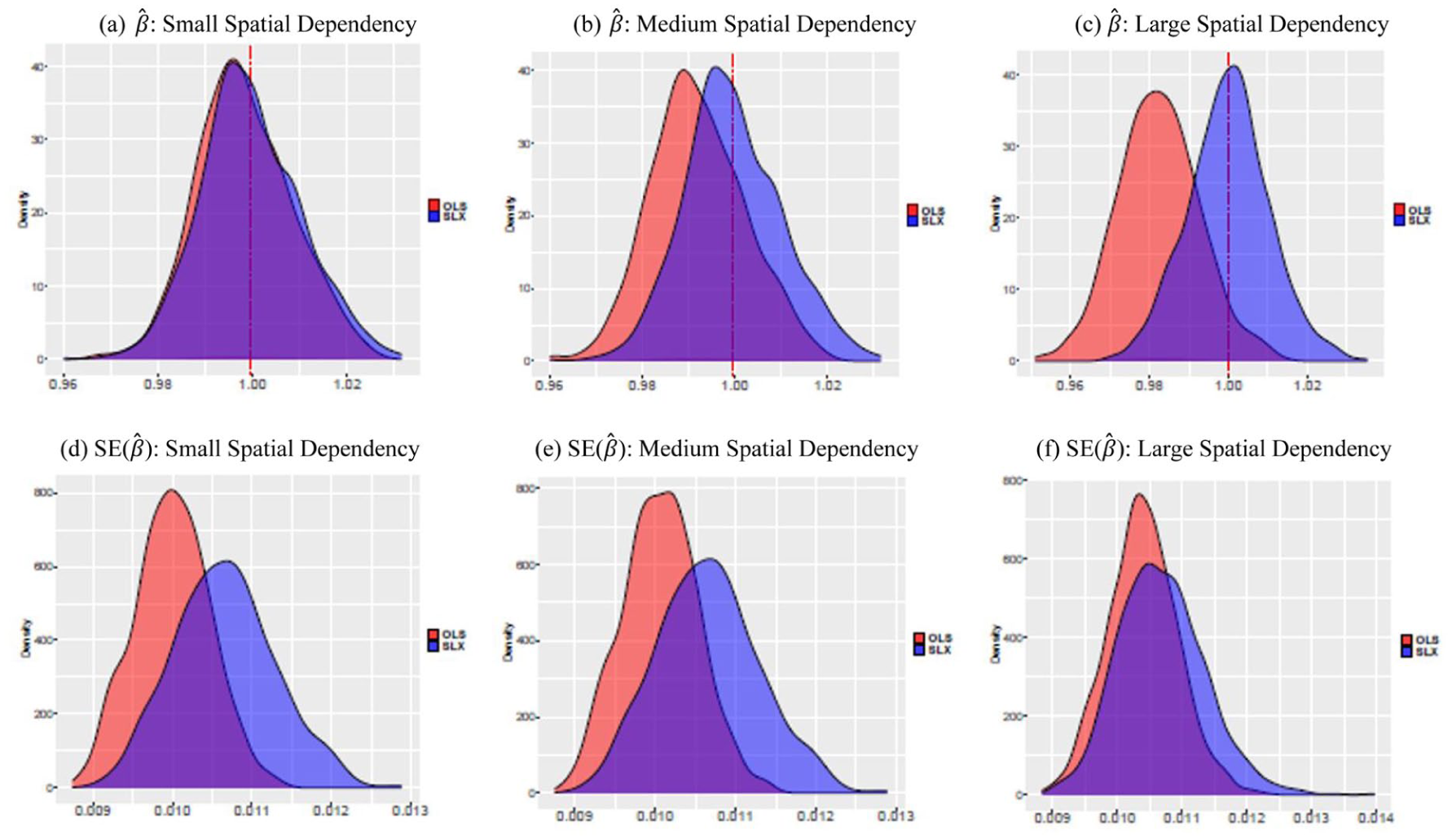
The (β) and SE (β) when spatial dependency increases: (a) $\overset{\land}{β}$ : small spatial dependency, (b) $\overset{\land}{β}$ : medium spatial dependency, (c) $\overset{\land}{β}$ : large spatial dependency, (d) SE( $\overset{\land}{β}$ ): small spatial dependency, (e) SE( $\overset{\land}{β}$ ): medium spatial dependency, and (f) SE( $\overset{\land}{β}$ ): large spatial dependency.

In this simulation, we set β = 1. However, as we will later show when discussing the consequences with real-world data, the findings in Figure 1 suggest that we may observe the opposite direction. For instance, we may obtain negative estimator values when the true β is positive, or vice versa, especially if we believe that our explanatory variable is expected to have a very small effect on crime. Furthermore, the risk of wrongly rejecting the null hypothesis also increases due to the ignorance of spatial dependency, which may lead to overconfidence in our estimator as it underestimates its uncertainty. In this paper, we focus on the SLX process for illustrative clarity and theoretical relevance for the study of crime. However, spatial dependencies may affect our analysis and hypothesis testing in various ways depending on the spatial dynamics inherent in our data. Spatial dependencies may exist in our dependent variable, independent variables, and even the error terms.

We report our next set of results for our second research question whether the empirical advantages of spatial model is robust to uncertainty in the definition of “nearby” areas. We present the models with no spatial lag in model (1) and those with lags by various distance cutoffs in models 2 to 5 in Supplemental Table A1. Of our primary interests, we displayed the results for the estimated coefficients and standard errors from no-spatial models, SLX models, and models with various misspecification rates for each increment of the distance cutoff. Specifically, we plot the densities of coefficient estimates and standard errors at varying levels of mis-specifications introduced and noted the coefficient values and standard errors for each distance cutoff for a comparison purpose. Our results yield patterns that are robust to different types of independent variables; therefore, we have chosen to highlight the representative patterns that can be inferred from the graph for % Homeowners, reported in Figure 2 for the estimated coefficients and Figure 3 for the standard errors. Figures for all other independent variables are reported in Supplemental Figures A1 to A8.

Figure 2.

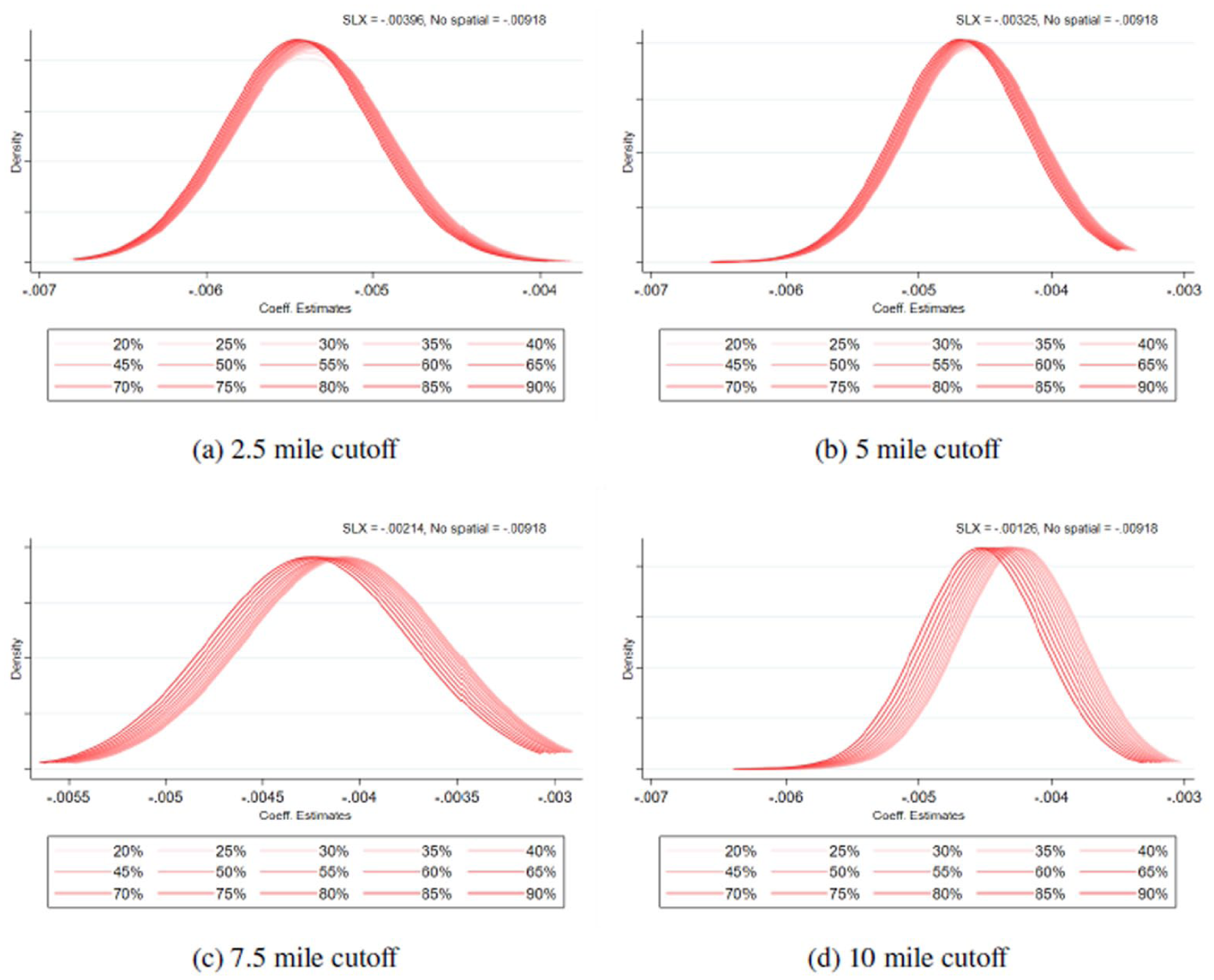
Coefficients with various misspecification probabilities in W based on inverse distance function in SLX models with different distance cutoffs: % Homeowners: (a) 2.5 mile cutoff, (b) 5 mile cutoff, (c) 7.5 mile cutoff, and (d) 10 mile cutoff.

Figure 3.

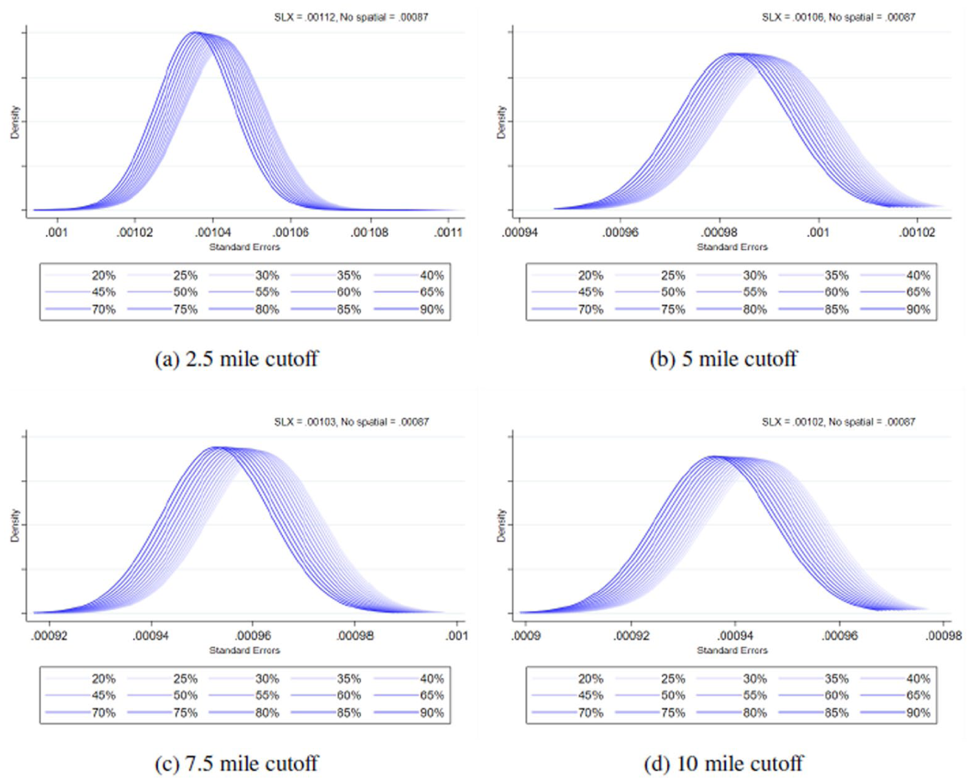
Standard errors with various misspecification probabilities in W based on inverse distance function in SLX models with different distance cutoffs: % Homeowners: (a) 2.5 mile cutoff, (b) 5 mile cutoff, (c) 7.5 mile cutoff, and (d) 10 mile cutoff.

There are a few important implications from the results. First, we found that as the misspecification probabilities in W increase, the coefficient density plots move further away from the SLX coefficient values. That is, as the uncertainty in measuring neighbors increases, the bias in β increases which is consistent with our theoretical expectation. However, we also observed that even with a high rate of misspecification in W, the bias is smaller than in the non-spatial models. For example, as shown in Figure 2a, the coefficient value estimated from the SLX model is about −0.004 whereas the coefficient densities from the models with various mis-specification rates in W are centered between −0.006 and −0.005. This suggests that the models with misspecified spatial matrix (about 25%–50% increase in magnitude compared to −0.005 and −0.006) overestimate the β for the measure of % Homeowners. Yet it is important to note that the non-spatial model is at greater risk of overestimation bias, as its coefficient for percent homeowners is approximately −0.009—about 1.25 times larger in magnitude than the corresponding estimate (−0.004) from the spatial model. This suggests that even with some degree of model misspecification or uncertainty in defining spatial dependence among units, the spatial modeling approach remains less susceptible to bias—in this case, the upward overestimation of the protective effect of homeownership. A similar pattern persists across different distance thresholds (ranging from 2.5 to 10 miles) used in constructing the spatial weight matrix.

Finally, we turn to our findings for the standard errors. We found that as the misspecification probabilities in W increase, the density plots for the standard errors move downwards from the standard error from the SLX model. That is, as the uncertainty in defining neighbors increases, models tend to underestimate the standard errors as theoretically expected. Yet again, even with higher misspecification rates in W, underestimation seems smaller than that of the non-spatial model. For example, as shown in Figure 3a, the standard error estimated from the correctly specified SLX model is approximately 0.00112, whereas the density plots from models estimated with varying degrees of misspecification in the spatial weights matrix are centered between 0.00102 and 0.00105 (about 6% to 9% decrease). This pattern suggests that inaccuracies in defining spatial relationships among units tend to lead to systematic underestimation of standard errors, likely due to the model’s failure to fully capture the covariance structure induced by spatial dependence. In other words, when the spatial weights matrix does not accurately represent the true spatial connectivity, the resulting parameter uncertainty is artificially suppressed. Yet, it is important to note that the non-spatial model exhibits an even greater degree of underestimation with a standard error of approximately 0.00087. This underscores that the omission of spatial dependence entirely—rather than merely specifying it imperfectly—poses a higher risk of biasing inferential precision. Collectively, these findings highlight the importance of incorporating spatial structure, even under conditions of moderate misspecification, as doing so yields more reliable estimates of uncertainty and reduces the risk of overconfident statistical inference.

Discussion

In the current study, we provide theoretical discussion why it is reasonable to assume that there are spatial spillover effects among neighborhood units when studying neighborhoods and crime. We also recognized that prior work has recognized the importance of accounting for the nearby area effects and has incorporated various methodological approaches to address spatial dependency in the study of neighborhoods and crime. Furthermore, we have provided a methodological discussion that ignoring the spatial dependency results in bias in the estimated β and inaccurate estimation in standard errors. In addition, we acknowledged another important challenge in defining neighbors in studies of spatial crime patterns is the methodological uncertainty regarding how to specify “neighbors” in a study of spatial crime patterns. That is, it is not readily clear to what spatial extent we can define neighboring areas for a given focal neighborhood. This uncertainty about the precise definition of neighbors can lead researchers to question whether spatial models are preferable for neighborhood and crime studies.

Although many studies have examined neighborhoods and crime while accounting for spatial dependency, less attention has been paid to providing empirical evidence on whether the spatial modeling approach is preferred. Therefore, we provide an in-depth theoretical and methodological discussion on the importance of addressing spatial dependency in the neighborhood and crime study context. At the same time, we empirically demonstrate how neglecting spatial spillover can lead to less accurate and efficient estimates of coefficients and standard errors, which may eventually result in bias in hypothesis testing.

The primary goal of this study was not to claim that spatial modeling is a novel approach. The methodology is well established, and prior research on spatial crime patterns has applied various spatial modeling strategies to address spatial dependence. Yet, despite its widespread use, less attention have been paid to explicitly and systematically demonstrate—through empirical evidence—that failing to account for spatial dependence can fundamentally alter research conclusions in neighborhood crime studies. Through simulation experiments as well as analyses using real crime data, we show that overlooking spatial effects can lead not only to shifts in the direction of estimated relationships but also to distortions in their magnitude.

Moreover, our findings also suggest that despite uncertainty in defining neighbors (or defining the W matrix), a kind of spatial modeling approach outperforms the non-spatial models. Even with a higher rate of misspecification introduced in the W, the bias in $\overset{\land}{β}$ and underestimation of standard errors are still smaller than those from the non-spatial models. Therefore, accounting for spatial dependency (even with potential errors in defining neighbors in the W) may be less susceptible to the risk of false hypothesis testing than omitting spatial terms altogether. This encourages the estimation of spatial models for a neighborhood and crime study, even with uncertainty and imperfect information for defining what constitutes nearby areas for a given neighborhood.

One important contribution of the current study is that it empirically demonstrates that ignoring spatial dependence can flip effect directions, distort effect sizes, and inflate statistical significance—ultimately producing biased and overconfident estimates. Such errors risk reinforcing false findings in the literature (publication bias) and misguiding crime policy by overlooking spatial spillovers. Our findings show that neglecting spatial dependence can not only inflate estimates but also reverse their signs producing misleading inferences that may reinforce false findings in the literature—a potential source of publication bias. As discussions in Nature⁵ emphasize, publication bias arises when research producing statistically significant or theoretically expected results is more likely to be published, while null or contradictory findings remain unreported. Such biases distort the cumulative scientific record, overstate effect sizes, and limit reproducibility. In spatial criminology, ignoring spatial dependence structures may yield results that appear robust but are in fact artifacts of spatial autocorrelation. This dynamic not only parallels but potentially feeds into publication bias as inflated or incorrectly signed effects are more publishable than null findings. Importantly, the patterns we identify align with theoretical expectations derived from our linear algebra illustration and are validated using crime data commonly employed in neighborhood research. By providing systematic empirical evidence, we show that accounting for spatial dependence is essential for both valid inference and sound policy.

In our data-generating process, both the dependent and independent variables are randomly generated, and only the treatment (or determinant) is structured to exhibit geographical dependence. Consequently, the simulation isolates the pure effect of model misspecification: any bias or sign reversal arises solely from the model’s failure to account for spatial processes, rather than from inherent spatial correlations in the data, which in real-world contexts are generated by several systematic social, economic, and environmental factors and their spatial dependencies. Our reported results reflect the average (or median) bias across 1,000 Monte Carlo iterations. While this summary captures the expected behavior of the estimator under repeated sampling, individual realizations can deviate more substantially. In real-research settings—where researchers observe only one realization of the data—the true bias may be larger than the mean simulation result depending on the specific configuration of spatial dependence and noise. Thus, the modest average bias we report should be interpreted as a conservative estimate of potential distortion, not an upper bound.

To further illustrate, consider the example of homeownership (findings we presented in Figures 2 and 3). In criminological research, homeownership is widely regarded as a key indicator of residential stability and collective efficacy, both of which are central control mechanisms through which neighborhood structural characteristics influence crime. This variable directly relates to a question often raised by scholars and policymakers namely, “Are more residentially stable neighborhoods safer?” Moreover, homeownership inherently exhibits spatial structure: the residential stability of surrounding neighborhoods may influence crime probabilities in focal neighborhood through spillover effects. Theoretically, homeownership is expected to have a crime-protective effect, but recognizing spatial spillovers adds complexity to how this relationship operates across space.

Our results demonstrate this dynamic. When spatial dependence is ignored, the non-spatial model tends to overestimate the protective effect of homeownership suggesting an inflated sense of its impact on crime. In contrast, the SLX model, which explicitly accounts for spatial dependence, produces more accurate coefficient estimates and standard errors. This indicates that ignoring the stability of adjacent neighborhoods can lead to biased and overly confident protective effects of residential stability on crime. A similar but little different pattern is observed for poverty (Supplemental Figures A1 and A5), but in the opposite direction: the effect size in the spatial model is larger than that estimated by the non-spatial model. Without properly addressing spatial dependency, the non-spatial model tends to underestimate the crime-producing effect of poverty. This distinction carries important policy implications, as it highlights how neglecting spatial interdependence may obscure the true magnitude of social disadvantage in shaping neighborhood crime.

These empirical demonstrations and findings have important policy implications. First, they suggest that neighborhood-level interventions focusing solely on internal characteristics—such as promoting residential stability or improving any local conditions—may overlook the broader spatial context that shapes neighborhood safety. Policies that fail to consider the influence of surrounding areas risk overestimating the benefits of local residential stability while underestimating the persistence and diffusion of socioeconomic disadvantage. Second, recognizing spatial spillovers implies that efforts to reduce crime may be more effective when coordinated regionally rather than implemented in isolation. Programs targeting residential stability or poverty reduction should therefore be designed with cross-neighborhood interdependencies in mind addressing not only focal neighborhoods but also their spatial associations of influence. In sum, our results provide empirical support for the importance of accounting for spatial dependence, which refines both our understanding of neighborhood effects and the design of place-based policy interventions.

One remaining question is whether our findings may be generalizable to other regional contexts with different samples as we utilized the sample data of NYC at the block group level. This is because different study area contexts and spatial scales (micro to macro spatial units) may provide different implications. We encourage future research to examine if spatial modeling is empirically preferred using other sample data and other spatial units frequently employed in previous studies of spatial crime patterns (i.e., street segment, block, or even larger units such as tracts) and how patterns may vary across and identify what precisely causes such variations. We also recognize that unmeasured local factors—such as regional subcultures, informal social networks, or other contextual influences—may operate simultaneously across adjacent neighborhoods, thereby contributing to spatial correlations among them. These latent processes often transcend administratively defined boundaries, shaping neighborhood dynamics in ways that are not fully captured by conventional socio-demographic indicators. For instance, shared cultural norms, collective behaviors, or localized economic conditions can diffuse through space, producing correlated outcomes even in the absence of direct interaction.

We also acknowledge the potential concern regarding crime reporting bias in neighborhood-level crime studies. However, prior research (e.g., Baumer, 2002) suggests that underreporting tends to be less problematic for more serious crime types. Our outcome variables are based on Uniform Crime Report (UCR) Part I offenses, which include the six most serious categories of crime, thereby minimizing the influence of differential reporting across neighborhoods. We also recognize the possible boundary issue that may arise when aggregating crime data to neighborhood units. Although addressing this issue is beyond the primary scope of our modeling objectives—and warrants a dedicated methodological study—spatial modeling provides a useful framework for mitigating its effects. Specifically, by incorporating spatially lagged terms for crime, researchers can partially account for boundary-induced spatial spillovers and improve the robustness of parameter estimates.

Also, we utilized an SLX approach as it is one of the most common and widely employed modeling strategies in neighborhood and crime studies. Yet, one remaining question is whether our findings remain similar when employing other types of spatial models such as the spatial lag model (SLM) or spatial error model (SEM). It is worth testing how other spatial modeling types may produce similar/different results compared to the one tested in the current study and discuss why so. In conclusion, we highlighted the theoretical and methodological importance of incorporating spatial modeling for a neighborhood and crime study. We also demonstrated that disregarding the spatial modeling approach may bring about bias in coefficients, inefficient standard errors, and thus potentially less precise and reliable hypothesis tests and confidence intervals. Our results confirmed our expectations that the spatial modeling approach is empirically preferred even with the presence of varying amounts of uncertainty in defining neighbors (or defining the W matrix).

Supplemental Material

sj-docx-1-cad-10.1177_00111287261416406 – Supplemental material for Spatial Modeling in Neighborhood and Crime Studies: An Empirical Examination

Supplemental material, sj-docx-1-cad-10.1177_00111287261416406 for Spatial Modeling in Neighborhood and Crime Studies: An Empirical Examination by Young-An Kim and Jongwoo Jeong in Crime & Delinquency

Footnotes

Declaration of Conflicting Interests

The authors declared no potential conflicts of interest with respect to the research, authorship, and/or publication of this article.

Funding

The authors received no financial support for the research, authorship, and/or publication of this article.

ORCID iD

Young-An Kim

Supplemental Material

Supplemental material for this article is available online.

Notes

Author Biographies

Young-An Kim is an Associate Professor in the College of Criminology and Criminal Justice at Florida State University, also a Faculty Affiliate at the Spatial Data Science Center (SDSC) at Florida State University. His research interests focus on various areas such as neighborhoods and crime, criminology of place, spatial analysis, immigration and crime, and quantitative research methods.

Jongwoo Jeong is an Assistant Professor of Political Science at Georgia State University. Grounded in political behavior, his research integrates perspectives from institutional analysis, public administration, and the politics of crime and criminal justice. Methodologically, he employs a broad range of approaches, including text-as-data methods, experimental design, causal inference, geographic and geopolitical analysis, and computational social science.

References

Anselin

(1988). Spatial econometrics: Methods and models. Springer.

Anselin

(2002). Under the hood issues in the specification and interpretation of spatial regression models. Agricultural Economics, 27(3), 247–267.

Anselin

Cohen

Cook

Gorr

Tita

(2000). Spatial analyses of crime. Criminal Justice, 4(2), 213–262.

Baller

R. D

Anselin

Messner

S. F.

Deane

Hawkins

D. F.

(2001). Structural covariates of us county homicide rates: Incorporating spatial effects. Criminology, 39, 561–588.

Baumer

E. P.

(2002). Neighborhood disadvantage and police notification by victims of violence. Criminology, 40(3), 579–616. https://doi.org/10.1111/j.1745-9125.2002.tb00967.x

Bernasco

Block

(2011). Robberies in Chicago: A block-level analysis of the influence of crime generators, crime attractors, and offender anchor points. Journal of Research in Crime and Delinquency, 48(1), 33–57.

Betz

Cook

S. J.

Hollenbach

F. M.

(2021). Bias from network misspecification under spatial dependence. Political Analysis, 29(2), 260–266.

Boessen

Hipp

J. R.

(2015). Close-ups and the scale of ecology: Land use and the geography of social context and crime. Criminology, 53(3), 399–426.

Boyd

Richerson

P. J.

(1985). Culture and the evolutionary process. The University of Chicago Press.

10.

Browning

C. R.

Feinberg

S. L.

Dietz

R. D.

(2004). The paradox of social organization: Networks, collective efficacy, and violent crime in urban neighborhoods. Social Forces, 83(2), 503–534.

11.

Cohen

Tita

(1999). Diffusion in homicide: Exploring a general method for detecting spatial diffusion processes. Journal of Quantitative Criminology, 15(4), 451–493.

12.

Cook

S. J.

Hays

J. C.

Franzese

R. J.

(2023). STADL up! The spatiotemporal autoregressive distributed lag model for TSCS data analysis. American Political Science Review, 117(1), 59–79.

13.

Felson

Boba

(2010). Crime and everyday life. SAGE Publications.

14.

Griffth

D. A.

(1996). Spatial autocorrelation and eigenfunctions of the geographic weights matrix accompanying geo-referenced data. Canadian Geographies, 40(4), 351–367.

15.

Haberman

C. P.

Ratcliffe

J. H.

(2015). Testing for temporally differentiated relationships among potentially criminogenic places and census block street robbery counts. Criminology, 53(3), 457–483.

16.

Hipp

J. R.

(2007). Block, tract, and levels of aggregation: Neighborhood structure and crime and disorder as a case in point. American Sociological Review, 72(5), 659–680.

17.

Hipp

J. R.

Kubrin

E. C.

(2017). From bad to worse: How changing inequality in nearby areas impacts local crime. RSF: The Russell Sage Foundation Journal of the Social Sciences, 3(2), 129–151.

18.

Hipp

J. R.

Perrin

A. J.

(2009). The simultaneous effect of social distance and physical distance on the formation of neighborhood ties. City & Community, 8(1), 5–25. https://doi.org/10.1111/j.1540-6040.2009.01267.x

19.

Hipp

J. R.

Roussell

(2013). Micro- and macro-environment population and the consequences for crime rates. Social Forces, 92(2), 563–595.

20.

Hipp

J. R.

J. C.

Kim

Y.-A.

(2017). Studying neighborhood crime across different macro spatial scales: The case of robbery in 4 cities. Social Science Research, 68, 15–29.

21.

Hunter

(1974). Symbolic communities: The persistence and change of Chicago’s local communities (Studies of urban society). University of Chicago Press.

22.

Janowitz

(1952). The community press in an urban setting (Glencoe, Ill). Free Press, 3, 473–493.

23.

Kim

Y.-A.

Hipp

J. R.

(2020). Street egohood: An alternative perspective of measuring neighborhood and spatial patterns of crime. Journal of Quantitative Criminology, 36, 29–66.

24.

Lee

J. Y.

Kwan

M.-P.

(2011). Visualisation of socio-spatial isolation based on human activity patterns and social networks in space-time. Tijdschrift voor economische en sociale geografie, 102(4), 468–485.

25.

LeSage

Pace

R. K.

(2009). Introduction to spatial econometrics. Chapman and Hall/CRC.

26.

Loftin

(1986). Assaultive violence as a contagious social process. Bulletin of the New York Academy of Medicine, 62(5), 550–555.

27.

Lynch

J. P.

Addington

L. A.

(2006). Understanding crime statistics: Revisiting the divergence of the NCVS and the UCR. Cambridge University Press.

28.

Mayhew

B. H.

Levinger

R. L.

(1976). Size and the density of interaction in human aggregates. American Journal of Sociology, 82(1), 86–110. http://www.jstor.org/stable/2777462

29.

Mears

D. P.

Bhati

A. S.

(2006). No community is an island: The effects of resource deprivation on urban violence in spatially and socially proximate communities*. Criminology, 44(3), 509–548.

30.

Messner

S. F.

Anselin

Baller

R. D.

Hawkins

D. F.

Deane

Tolnay

S. E.

(1999). The spatial patterning of county homicide rates: An application of exploratory spatial data analysis. Journal of Quantitative Criminology, 15(4), 423–450.

31.

Morenoff

J. D.

Sampson

R. J.

Raudenbush

S. W.

(2001). Neighborhood inequality, collective efficacy, and the spatial dynamics of urban violence. Criminology, 39(3), 517–559.

32.

Papachristos

A. V.

Wildeman

Roberto

(2015). Tragic, but not random: The social contagion of nonfatal gunshot injuries. Social Science & Medicine, 125, 139–150.

33.

Peterson

R. D.

Krivo

L. J.

(2010). Divergent social worlds: Neighborhood crime and the racial-spatial divide. Russell Sage Foundation.

34.

Ren

Kwan

M.-P.

(2009). The impact of the Internet on human activity–travel patterns: Analysis of gender differences using multi-group structural equation models. Journal of Transport Geography, 17(6), 440–450.

35.

Rengert

G. F.

Piquero

A. R.

Jones

P. R.

(1999). Distance decay reexamined. Criminology, 37(2), 427–446.

36.

Rick

(2009). From the ground up: Translating geography into community through neighbor networks. Princeton University Press.

37.

Rüttenauer

(2019). Spatial regression models: A systematic comparison of different model specifications using monte carlo experiments. Sociological Methods & Research, 51(2), 728–759.

38.

Sampson

R. J.

(2012). Great American city: Chicago and the enduring neighborhood effect. University of Chicago Press.

39.

Sampson

R. J.

Raudenbush

S. W.

Earls

(1997). Neighborhoods and violent crime: A multilevel study of collective efficacy. Science, 277(5328), 918–924.

40.

Weisburd

(2015). The law of crime concentration and the criminology of place. Criminology, 53(2), 133–157.

41.

Weisburd

Groff

E. R.

Yang

S.-M.

(2012). The criminology of place: Street segments and our understanding of the crime problem. Oxford University Press.

42.

J. C.

Hipp

J. R.

Boessen

(2016). Voluntary organizations and neighborhood crime: A dynamic perspective. Criminology, 54(2), 212–241.

Supplementary Material

Please find the following supplemental material available below.

For Open Access articles published under a Creative Commons License, all supplemental material carries the same license as the article it is associated with.

For non-Open Access articles published, all supplemental material carries a non-exclusive license, and permission requests for re-use of supplemental material or any part of supplemental material shall be sent directly to the copyright owner as specified in the copyright notice associated with the article.

0.00 MB

0.98 MB