
Abstract
Research has consistently revealed a link between involvement in adolescent delinquency and adult criminal behavior. Even so, there remains much that is unknown about this association, including the potential mechanisms that might explain it. The current study sought to add to this literature by examining the connection between being arrested as a juvenile and future self-reported involvement in adult criminal behavior. To do so, we analyzed data drawn from the National Longitudinal Study of Adolescent to Adult Health (Add Health). We employed propensity score matching analysis to examine whether participants who were arrested as juveniles had significantly different mean scores on measures of crime (violent, nonviolent, and total) at two different points in adulthood when compared to matched controls. The results of these analyses revealed that participants who had been arrested as a juvenile self-reported greater involvement on four of the six crime measures compared to matched controls although these mean differences were attenuated once participants were matched on key covariates, including adolescent delinquency, low self-control, delinquent peers, and neuropsychological functioning, among others. We discuss the interpretation of these results and draw attention to the role that labeling may play in accounting for the link between juvenile arrests and adult criminal involvement.
Introduction
The stability of antisocial behavior over the life course is one of the most consistent and robust findings to emerge from the criminological literature (Cairns & Cairns, 1994; Gottfredson & Hirschi, 1990; Wright et al., 2015). Children who engage in age-inappropriate behaviors are at-risk for developing into adolescents who engage in delinquency who, in turn, are at risk for becoming adults who commit criminal acts (Wright et al., 2015). Indeed, the best predictor of future misbehavior is a history of misbehavior (Tracy et al., 1990). As a result, it is not surprising that the vast majority of adult criminal offenders have a history of antisocial behavior that dates back to adolescence and even childhood (Benson, 2013). And, stability in antisocial behaviors is most likely to occur in the tails of the distribution—that is, the “worst of the worst” are the least likely to change their behaviors, and they are precisely the offenders who commit the majority of serious violent offenses (DeLisi, 2005).
The association between prior antisocial behavior and future antisocial is so well-established that it could be considered one of the few axiomatic laws within the criminological literature (Wright et al., 2010). Despite mounds of evidence underscoring the stability in antisocial behaviors, the mechanisms that are responsible for creating this stability have remained somewhat elusive and remain a matter of disagreement (Nagin & Paternoster, 2000). Some explanations, for example, have focused on lifestyle factors, some have focused on latent traits and other individual differences, and still others have focused on the social consequences that emanate from engaging in antisocial behaviors that embed individuals within criminogenic contexts (Gottfredson & Hirschi, 1990; Moffitt, 1993; Sampson & Laub, 1993; Wright et al., 2010). Another intriguing explanation that has been advanced is that labeling may be particularly salient for understanding the stability of antisocial behaviors over time (Sampson & Laub, 1992). The current study sought to address the possibility that labeling is involved in behavioral stability by examining males and females drawn from a nationally representative and longitudinal sample of adolescents.
Explanations of Behavioral Stability
A number of theoretical explanations have been consistently applied to explain stability in antisocial behaviors across different segments of the life course. These explanations can be broadly grouped into two overarching perspectives. The first perspective is known population heterogeneity (Nagin & Paternoster, 2000). This approach focuses on criminogenic traits or other individual differences in propensities that are thought to cause antisocial behaviors (Gottfredson & Hirschi, 1990; Wilson & Herrnstein, 1985). These traits/propensities are differentially distributed across people and thus people engage in crime and other forms of antisocial behaviors at different rates. At the same time, according to the population heterogeneity perspective, the traits/propensities that cause antisocial behaviors are typically viewed as being relatively stable throughout most of the life course. Since these traits cause antisocial behaviors, and since these traits are relatively stable, then the antisocial behaviors that are caused by the traits are relatively stable over time as well.
Perhaps the most well-known criminological theory that fits within the population heterogeneity perspective is Gottfredson and Hirschi’s (1990) low self-control theory. According to this theory, all crime, delinquency, and other forms of antisocial behaviors are the result of relatively low levels of self-control (in tandem with an opportunity). Since low levels of self-control are the cause of antisocial behaviors, all other correlates to crime are not causal, but rather are spuriously associated. A substantial amount of research has tested this part of the theory and the results have revealed support in favor of the theory (Pratt & Cullen, 2000; Vazsonyi et al., 2017; Tehrani & Yamini, 2020). Gottfredson and Hirschi’s theory also provides an explanation as to why antisocial behaviors are relatively stable. Specifically, they argued that low self-control is created by parental socialization and the level of self-control becomes relatively fixed by around the age of 12. Because variation in self-control is the cause of crime and antisocial behaviors, and because self-control remains relatively from early adolescence onward, the antisocial behaviors that are created by variation in self-control should remain relatively stable as well. Research has also tested the “stability hypothesis” extracted from their theory and the results of these studies have shown that levels of self-control remain relatively stable for most people (Coyne & Wright, 2014; Jo & Zhang, 2012; Turner & Piquero, 2002).
In stark contrast to the population heterogeneity perspective is the state dependence perspective. According to the logic of the state dependence perspective, stability in antisocial behavior occurs because initially engaging in a criminal act frequently creates a cascade of transformations in local life circumstances (Nagin & Paternoster, 2000). For example, committing crime likely reduces contact and exposure to prosocial persons, could result in unemployment, and may embed the offender in a criminalistic lifestyle that is typified by contact with antisocial peers, living in a disadvantaged community, and residing in poverty. These transformations work to increase the odds of future criminal involvement, a cycle that continues to repeat and results in the stability of antisocial and criminal behaviors over long swaths of the life course.
Sampson and Laub’s (1993) age-graded theory of informal social control is the theoretical perspective most often equated with state dependence in criminology. They argue that offenders become knifed off from conventional society when they engage in criminal behaviors. By losing bonds to conventional society, they are likely to persist with their criminal behavior in the future because they lack stakes in conformity and because they have less to lose from committing crimes. This explanation is in line with Lemert’s (1951, 1972) conceptualization and description of secondary deviance (Sampson & Laub, 1992). Specifically, secondary deviance is viewed as being part of a labeling process wherein once an individual engages in criminal behavior—and has been identified—a series of formal and informal reactions begin to occur. Their criminal label may prevent them from entering into conventional roles and may be significant obstacles to opportunities that are viewed as being necessary for being successful. These reactions may be at the institutional level and they also occur in individualized settings, where their criminal label causes them to be stigmatized, ostracized, and embedded in criminogenic environments and lifestyles. In short, the initial criminal act produces downstream criminogenic effects that make the stability of crime and antisocial behavior likely.
Current Study
Although there has been a long line of research testing various predictions derived from state dependence in general and Sampson and Laub’s (1993) theory specifically, there is a lack of research examining whether secondary deviance (labeling) may be responsible for producing stability in criminal behavior over the life course. Certainly, there has been research examining labeling as part of the reason why the risk for reoffending is so high (Chiricos et al., 2007; Liberman et al., 2014), but whether secondary deviance can explain part of the reason for the stability in criminal behavior when ruling out alternative explanations has been difficult to achieve. Part of the reason for this lack of research is because the labeling process typically has to be inferred once other rival explanations have been ruled out. As a result, the ability to identify labeling processes is contingent on whether the analytical strategy has effectively accounted for all other competing explanations which is not always the case. The current study sought to build upon this previous research by using an analytical approach that is capable of accounting for alternative explanations (i.e., population heterogeneity and state dependence) and thus is able to help isolate the effects of labeling from these alternative interpretations. Specifically, we estimated propensity scores matching (PSM) models to examine whether being arrested as a juvenile was associated with self-reported crime and delinquency throughout adolescence and into adulthood after taking into account measures derived from other explanations of behavioral stability. PSM is uniquely situated to address these issues as it is able to help isolate whether a juvenile arrest is associated with adult criminal behavior before and after accounting for the key measures derived from population heterogeneity and state dependence. If being arrested as a juvenile increases involvement in criminal behavior in adulthood even after accounting for (i.e., matching on) key measures drawn population heterogeneity and state dependence, then these results would be consistent with a labeling interpretation. However, if being arrested is not associated with adulthood criminal involvement after accounting for key measures from population heterogeneity and state dependence, then processes that are in line with these perspectives are likely a more viable interpretation of the results.
Methods
Data
Data for this study were drawn from the National Longitudinal Study of Adolescent to Adult Health (Add Health) (Udry, 2003). The Add Health is an ongoing, longitudinal, and nationally representative sample of middle and high school students during the 1994 to 1995 school year. All students attending one of the schools selected for inclusion in the study were administered a self-report survey on a specified school day. These surveys covered a wide range of topics, including topics related to family, peers, and school. Overall, about 90,000 adolescents participated in what is known as the Wave 1 in-school component of the study. A subsample of these participants was then selected to be reinterviewed in their homes (along with their primary caregiver) and asked more extensive questions, including questions that addressed sensitive topics. Youth, for instance, were asked about their involvement in acts of delinquency, their victimization experiences, and their social relationships. A total of 20,745 adolescents and 17,700 of their primary caregivers participated in what is known as the Wave 1 in-home component of the study (Harris et al., 2003).
The second wave of data collection occurred approximately one-and-a-half years after the initial data collection began. At this time, most of the participants were still adolescents and so the survey instruments remained relatively similar between waves. For instance, participants were asked about their involvement in risky sexual behaviors, their use of drugs and alcohol, and their relationships with their family and friends. In total, 14,738 adolescents participated in the Wave 2 component of the study. The third wave of data was collected in 2001 to 2002. At this data collection wave, most of the participants were young adults and, as a result, the questions asked and the topics covered were amended to be more reflective of this point in the life course. Participants, for example, were asked about their educational achievements, their employment, and their marriages. Overall, there were 15,197 participants included in the Wave 3 component of the study. In 2007 to 2008 the fourth wave of data was collected when most of the participants were in their late 20s and early 30s. At this wave, participants were asked questions that covered a wide range of topics germane to adulthood, including questions about their contact with the criminal justice system, their financial well-being, and their social relationships. A total of 15,701 participants were included in the Wave 4 component of the study.
Measures
Treatment Variable
Whether the participant had been arrested prior to their 18th birthday was the treatment variable for the study. Specifically, at Wave 3, participants were asked how many times they were arrested before they were 18 years old. For this study, responses to this question were recoded to be dichotomous, such that 0 = never arrested prior to turning 18 years old and 1 = arrested at least one time prior to turning 18 years old.
Outcomes
Six outcome measures were included in the study, all of which measured involvement in criminal behavior during adulthood. The first three measures were created from Wave 3 data. Specifically, a Wave 3 nonviolent criminal behavior scale was created, a Wave 3 violent criminal behavior scale was created, and a Wave 3 total criminal behavior scale was created. The Wave 3 nonviolent criminal behavior consisted of six items that measured involvement in acts of nonviolent offenses, such as damaging property and selling drugs (α = .68). The Wave 3 violent criminal behavior scale consisted of five items that indexed the degree to which participants were involved in violent acts of criminal behavior, including using a weapon in a fight and taking part in a group fight (α = .60). The Wave 3 total criminal behavior scale was created by summing together the Wave 3 nonviolent criminal behavior scale and the Wave 3 violent criminal behavior scale (α = .73). The next three outcome measures were duplicates of those created at Wave 3, but used Wave 4 data instead. In particular, the Wave 4 nonviolent criminal behavior scale consisted of eight items (α = .62), the Wave 4 violent criminal behavior scale consisted of five items (α = .60), and the Wave 4 total criminal behavior scale consisted of 13 items (α = .57). These scales have been used in previous research analyzing the Add Health data (Bekbolatkyzy et al., 2019).
Covariates
Ten covariates were used to create the propensity score. First, a total adolescent delinquency scale was included that is identical to a scale that has been used previously (Bekbolatkyzy et al., 2019). At Wave 1, participants were asked about their involvement in 15 acts of nonviolent and violent delinquency, including how frequently they were part of a physical fight, how often they had stolen something worth more than $50, and how often they had sold drugs during the previous 12 months. Responses to these items were summed to create the total adolescent delinquency scale (α = .84).
Second, a low self-control scale was included in the analyses. At Wave 1, participants responded to 23 different questions that measured individual variation in self-control. Specifically, participants were asked whether they had trouble keeping their mind focused and whether they would go with their “gut feelings” without reflecting too much about the consequences. Responses to these items were then summed with higher values indicating lower levels of self-control (α = .76). This scale is identical to the scale that has been used previously (Beaver et al., 2009).
Third, a delinquent peers scale was included in the analyses. At Wave 1, participants were asked three questions that measured their exposure and contact with delinquent peers. Specifically, they were asked how many of their three closes friends smoked marijuana more than once per month, consumed alcohol at least once per month, and smoked at least one cigarette per day. Responses to these items were summed with higher values reflecting a greater number of delinquent peers (α = .76). This scale has been used previously (Bellair et al., 2003).
Fourth, an adolescent victimization scale was included. At Wave 1, participants were asked to indicate how often in the preceding 12 months they had been show by someone, stabbed by someone, jumped by someone, or had a knife or gun pulled on them. Responses to these items were summed to create the victimization scale (α = .61). This scale and variants of it have been used previously (Alua et al., 2024; Haynie & Piquero, 2006; Mammadov et al., 2021)
Fifth, a measure of neuropsychological functioning was included. At Wave 1, participants completed an abbreviated version of the Peabody Picture Vocabulary Test, a test which has been shown to be a valid and reliable way to measure verbal aptitude and receptive vocabulary (D’Amato et al.’ (1988); Dunn & Dunn, 1981). Measures of verbal skills have been used to measure neuropsychological functioning and this exact measure has been used previously among researchers analyzing the Add Health to measure variation in neuropsychological functioning (Beaver et al., 2011). Importantly, higher scores on this variable reflect better neuropsychological functioning.
Sixth, a criminal mother variable was included. At Wave 4, participants were asked whether their biological mother had spent time in prison or jail. This variable was coded dichotomously (0 = no, 1 = yes), and this same measure has been used previously (Diana et al., 2023).
Seventh, a criminal father variable was included. At Wave 4, participants were asked whether their biological father had spent time in prison or jail. This variable was coded dichotomously (0 = no, 1 = yes), and this same measure has been used previously (Diana et al., 2023).
Eighth, gender was measured at Wave 1 and was included as a binary variable, wherein 0 = female and 1 = male.
Ninth, age was measured at Wave 1 and was created by using the participant’s birthdate along with the date that the interview was completed.
Tenth, race was based on three categories: White, Black, and Other Race.
Plan of Analysis
The analysis for this plan was centered on propensity score matching (PSM). PSM is a statistical approach that attempts to mimic a randomized control experiment with observational data (Guo & Fraser, 2010). To do so, participants are assigned to one of two groups: either a treatment group or a control group. Those in the treated group are then individually matched to another participant who is in the control group who has a similar “propensity” to have been treated, but was not. In the current study, the treatment group consists of participants who had been arrested prior to their 18th birthday while the control group consists of participants who had not been arrested prior to the age of 18. Participants were matched based on their propensity scores that were generated using the ten covariates described above and the outcome measures were then compared between participants from the treated and control groups to determine whether there are average differences between the two groups. Matching was accomplished by using one-to-one nearest neighbor with a .05 caliper (without replacement).
Results
We begin our analysis by examining mean differences between participants who had been arrested before the age of 18 and those who had not been arrested prior to the age of 18. Table 1 presents the results of these analyses. The left-hand columns of the table depict the average differences for the unmatched sample—that is, these are the differences that exist between the two groups without employing PSM. Of the ten covariates, all but race differed significantly between the treated and control groups. The right-hand side of the table shows mean differences after matching on propensity scores. As can be seen, there were no statistically significant differences in the means between the matched and control groups. These null effects indicate that the matching procedure worked as it eliminated statistically significant differences that existed prior to matching.
Mean Values for Pre- and Post-Matching to Examine Covariate Balance.
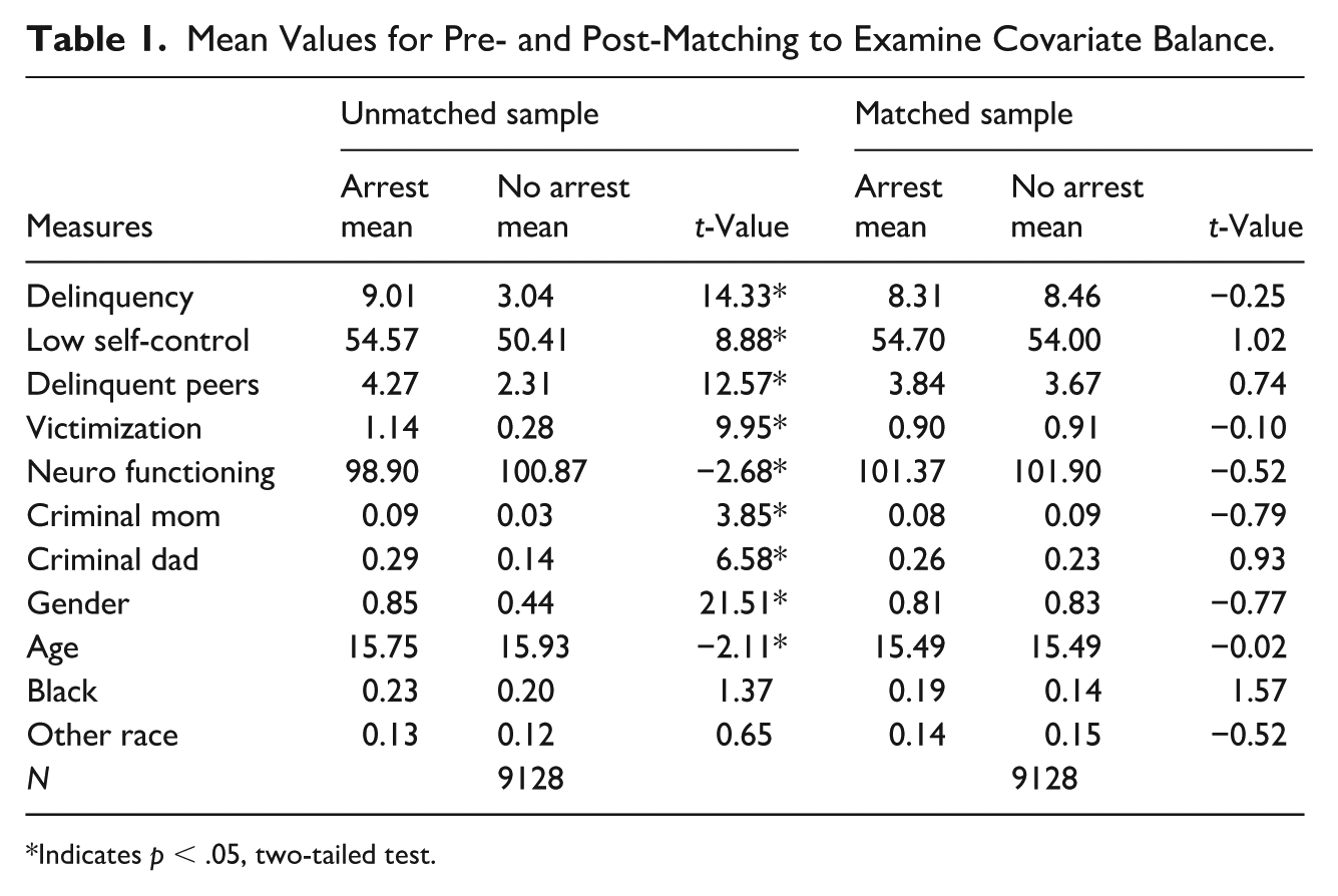
Indicates p < .05, two-tailed test.
With the two groups comparable on the covariates, it is now possible to examine whether the outcome measures differed after they have been matched on the covariates. Table 2 contains the results of these analyses. Once again, the results of the analyses for the unmatched sample are contained on the left-hand side of the table. These findings show statistically significant average differences between the treated and control groups on all six of the outcome measures. The right-hand side of the table shows the findings of the matched sample. Two results are particularly noteworthy. First, in these analyses, only four of the six outcome measures differed significantly between the treated and control groups. Second, of the four statistically significant differences, the differences were attenuated considerably when compared to the differences that existed in the unmatched sample. For example, in the unmatched sample, t-values ranged between 10.16 and 21.05 for these four measures, but the t-values only ranged between 2.37 and 5.42 in the matched sample for these four measures.
Pre- and Post-Matching t-tests Examining the Effect of being Arrested as a Juvenile on Adult Criminal Behavior.
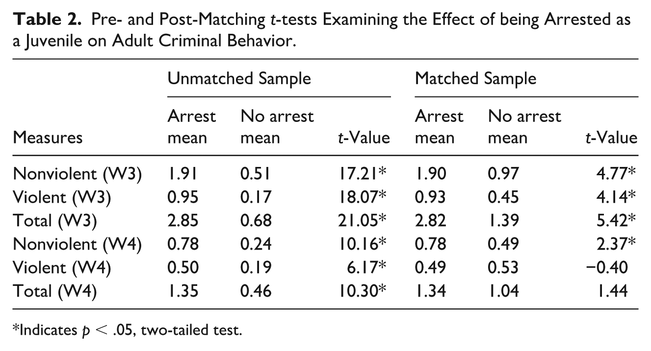
Indicates p < .05, two-tailed test.
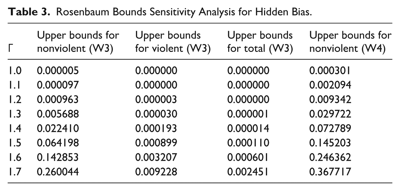
Last, we conducted sensitivity analysis to help determine the robustness of the statistically significant average differences that were detected in the matched sample. To do so, we calculated Rosenbaum bounds which are often used as a way to determine the degree to which hidden bias (or excluded confounders) may account for the statistically significant average differences that were detected in the matched sample (Rosenbaum, 2005). The interpretation of Rosenbaum bounds centers largely on Γ, a parameter that in this study indicates how much more likely participants in the treatment group would have to be arrested when compared to their matched control in order for the statistically significant mean differences to become null. Table 3 portrays the results of these analyses and show change in p-values that corresponds to an increase in Γ. For the Wave 3 nonviolent criminal behavior scale, the statistically significant difference that existed in the matched sample would disappear if a treated participant was about 1.5-1.6 times more likely to be arrested than their matched control because of unmeasured confounders. For Wave 3 violent criminal behavior and Wave 3 total criminal behavior, the value of Γ would have to exceed 1.7 in order for the statistically significant differences to become null. Last, for the statistically significant differences between the treatment and matched control groups for Wave 4 nonviolent criminal behavior would disappear if Γ was around 1.4-1.5.
Rosenbaum Bounds Sensitivity Analysis for Hidden Bias.
Discussion
Given that a relatively small proportion of all offenders account for the majority of all violent criminal offenses (DeLisi, 2005), it stands to reason that identifying these offenders would be particularly important for reducing criminal involvement. Moreover, these serious violent offenders tend to begin offending very early in the life course and then persist with their criminal behaviors throughout the life course (Moffitt, 1993). Identifying and understanding the mechanisms that might contribute to the stability in criminal behavior could go a long way towards creating policies and programs that might be able to disrupt behavioral stability and help to propel offenders onto a prosocial pathway. Although numerous explanations have been advanced to understand the stability in criminal behavior (Gottfredson & Hirschi, 1990; Sampson & Laub, 1993), and even though a large body of research has empirically examined the merits of these explanations, there still remains relatively little consensus on the underlying reasons for criminal stability (Wright et al., 2010). The current study sought to add to this literature by examining the connection between being arrested as a juvenile and self-reported involvement in crime and delinquency in adulthood. Analysis of the data revealed two key findings.
First, and not surprisingly, there were statistically significant mean differences across all of the covariates (except for race) between participants who had been arrested as a juvenile and those who had not been arrested as a juvenile. Keep in mind that we examined a wide range of covariates that have been previously linked to the development and persistence of criminal behavior, including self-reported delinquency, low levels of self-control, exposure to delinquent peers, and neuropsychological functioning, among others. Indeed, the included covariates cover most of the key explanations for behavioral stability. Just as importantly, however, was that all of these statistically significant mean differences were eliminated during the matching sample. After we employed PSM techniques, none of these previous covariates differed significantly between the arrested (treated) group and the non-arrested (control) group.
Second, prior to matching, there were statistically significant mean differences between participants who had been arrested as a juvenile and those who had not been arrested as a juvenile for all six of the self-reported criminal involvement scales at Waves 3 and 4. Again, not surprisingly, participants who had been arrested as a juvenile scored significantly higher on self-reported nonviolent criminal behavior (Waves 3 and 4), violent criminal behavior (Waves 3 and 4), and total criminal behavior (Waves 3 and 4) when compared to participants how had not been arrested as a juvenile. Of particular interest, however, were the mean differences on these six self-reported criminal behavior scales in the matched sample. Interestingly, after participants had been successfully matched, there were not any significant differences between the arrested and non-arrested groups for the Wave 4 violent criminal behavior scale and the Wave 4 total criminal behavior scale. The mean differences for the remaining four criminal behavior scales (all three at Wave 3 and the nonviolent criminal behavior scale at Wave 4) were significantly different between the two groups, but these differences were substantially reduced.
Given these results, the question remains how they should be interpreted? Remember that the PSM models included covariates that were designed to tap the key constructs derived from the most widely applied and verified explanations for the stability of criminal behavior. The included measures tapped explanations from Gottfredson and Hirschi’s (1990) theory, Moffitt’s (1993) developmental taxonomy, social learning theory as well as items that accounted for genetic and family-wide criminogenic influences. Perhaps most importantly, however, was that we included a measure of total delinquency measured at Wave 1. This measure captures all (or most) of the risk factors that initially caused a participant to engage in delinquency. In other words, the Wave 1 total delinquency scale is a catch-all measure that included all of the criminogenic influences that were pertinent to why the adolescent committed delinquency. This is particularly important for this study since we were measuring differences between participants who had been arrested as a juvenile those who had not. Since arrests are largely a function of criminal and delinquent involvement (Barnes, 2014; DeLisi, 2010), including this Wave 1 total delinquency scale should have captured the most salient criminogenic factors that differed between those who had been arrested as a juvenile and those who had not been arrested as a juvenile. Successfully matching on this Wave 1 total delinquency scale along with all of the other covariates included in the study should have provided a very stringent analysis.
Even with this conservative approach employed, the fact that four of the six self-reported adult criminal behavior scales differed significantly between the groups strongly suggests that there is something criminogenic about being arrested as a juvenile that contributes to stability in criminal behavior—at least into early adulthood—above and beyond typically measured criminogenic influences. While admittedly speculative, these results are consistent with a secondary deviance explanation or labeling more generally, wherein once an individual is arrested there are processes at play that may not be entirely measurable and have to be inferred via ruling out alternative explanations. In this case, perhaps juveniles who are arrested become known to law enforcement and are more likely to be arrested when a crime occurs in their neighborhood or perhaps juveniles who are arrested are subject to forms of discrimination that further embed them in a criminalistic lifestyle. The number of explanations that could be applied to explain this stability are in many ways limitless, but appear to be most consistent with a state dependence approach to understanding criminal stability (Nagin & Paternoster, 2000).
Policy Implications
Precisely how these results should be used for treatment and policy are not necessarily clear-cut. On the one hand, they indicate that being arrested is associated with increased criminal involvement in adulthood. These findings, therefore, could be used to justify punitive sanctions because “get-tough” policies would incapacitate these offenders who appear to remain involved in crime and delinquency even after being arrested. Keep in mind, however, that this might be too hasty of a conclusion as these statistical models did not provide any information about whether the participant received treatment as a part of their juvenile arrest (and potential conviction). Perhaps if this information was available, then it would have been possible to determine whether treatment and rehabilitation are able to attenuate the criminogenic effects of being arrested as a juvenile or may have even been beneficial by providing treatment services to at-risk youth. On the other hand, when comparing the results of the unmatched sample to the matched sample, it is clear that the criminogenic effects of being arrested as a juvenile are much less consistent and much less severe in the matched versus unmatched sample. These results suggest that perhaps having an adolescent criminal record does have a criminogenic effect (that cannot be explained by key covariates), but that it takes on less importance over time as other social and individual processes unfold through the maturation process. Regardless, there is no evidence available in the models that suggests being arrested for a crime as a juvenile is associated with reductions in future criminal involvement. This necessarily raises the possibility that perhaps taking a hands-off approach to adolescent offenders might lead to less crime, not more. While radical non-intervention approaches have been implemented previously (Miller, 1991; Schur, 1973), these approaches have not been shown to be effective at solving the crime and delinquency problem, and certainly have not been shown to be as effective as those that take a more treatment-oriented approach (Cullen, 2013; Travis & Cullen, 1984).
Limitations and Conclusions
Although this study provides some insight into the stability of criminal behavior, there are a number of limitations that need to be addressed in future research. First, the measure of juvenile arrest was a retrospective measure based on self-reports. Although self-reported criminal behavior has been shown to be valid and reliable (Thornberry & Krohn, 2000), this measurement approach nonetheless raises questions about the possibility that the results could be partially a function of recall bias. Second, even though covariates were included for most of the key explanations of criminal stability, PSM is a data-driven technique and thus the results are contingent on whether all of the appropriate covariates were included in the models. Based on the measured included to create the propensity scores, along with the results generated from the Rosenbaum bounds analysis, it appears as though the results are relatively robust, but replication research is needed to verify empirically the results reported here. Last, the Add Health is a nationally representative sample which makes these results generalizable to a large population, but whether these same findings would be detected in a criminal sample or other at-risk sample awaits future research.
The juvenile correction system is different than the adult criminal justice system and the focus is generally considered to be more progressive with a concerted effort to rehabilitate offenders and prevent future crime and delinquency. The results generated from this study suggest that the juvenile justice system does not necessarily reduce future criminal and delinquent involvement, but rather likely serves to further embed adolescents in a lifestyle where resorting to crime and delinquency is the norm. And, this effect is not confined solely to adolescence, but appears to extend into early adulthood. Understanding the precise ways that the juvenile justice system is criminogenic, and perhaps ways to correct these criminogenic effects, could go a long way towards making it truly rehabilitative for those who are processed through it, a goal that has been at the forefront of the juvenile justice system since its inception.
Footnotes
Acknowledgements
Wave VI of Add Health is supported by two grants from the National Institute on Aging (1U01AG071448, principal investigator Robert A. Hummer, and 1U01AG071450, principal investigators Allison E. Aiello and Robert A. Hummer) to the University of North Carolina at Chapel Hill. Co-funding for Wave VI is being provided by the Eunice Kennedy Shriver National Institute of Child Health and Human Development, the National Institute on Minority Health and Health Disparities, the National Institute on Drug Abuse, the NIH Office of Behavioral and Social Science Research, and the NIH Office of Disease Prevention. The content of this paper/presentation is solely the responsibility of the authors and does not necessarily represent the official views of the National Institutes of Health or the University of North Carolina at Chapel Hill. Add Health was designed by J. Richard Udry, Peter S. Bearman, and Kathleen Mullan Harris at the University of North Carolina at Chapel Hill. The project was funded by the Eunice Kennedy Shriver National Institute of Child Health and Human Development from 1994-2021, with cooperative funding from 23 other federal agencies and foundations. Add Health is currently directed by Robert A. Hummer; it was previously directed by Kathleen Mullan Harris (2004–2021) and J. Richard Udry (1994–2004).
Funding
The authors disclosed receipt of the following financial support for the research, authorship, and/or publication of this article: This article was prepared as part of the grant financing of scientific and (or) scientific and technical programs for 2024-2026, funded by the Science Committee of the Ministry of Science and Higher Education of the Republic of Kazakhstan (project AP23489588 “Improving the police service model in ensuring the safety of citizens in modern conditions”).
Declaration of Conflicting Interests
The authors declared no potential conflicts of interest with respect to the research, authorship, and/or publication of this article.