Leveraging Bayesian Statistics in Educational Leadership and Policy Studies

Abstract

Purpose

This paper examines the application of Bayesian statistics in educational leadership and policy studies. It explores the philosophical and methodological foundations, highlights the contributions to estimation thinking in quantitative research, demonstrates the implementation of Bayesian methods through a detailed case study, and proposes a heuristic for applying Bayesian techniques in educational research.

Research Approach

Building on the methodological discussion, this study presents a case study to illustrate the practical application of Bayesian statistics. The analysis investigates the relationship between teachers’ perceptions of school climate and their job satisfaction in U.S. middle schools, utilizing data from the 2018 Teaching and Learning International Survey. A Bayesian multilevel modeling approach is employed to analyze the data, incorporating Markov chain Monte Carlo (MCMC) techniques for estimating posterior distributions. Predictive mean matching is used for data imputation to address missing data.

Findings

The case study demonstrates that teachers’ job satisfaction is positively associated with better teacher-student relations and greater participation among stakeholders, while a better disciplinary climate is associated with higher job satisfaction. The Bayesian method yields robust statistical insights, demonstrating its advantages in estimation thinking and inferences.

Implications for Research and Practice

The findings suggest that Bayesian statistics can enhance methodological rigor and offer practical insights in educational leadership and policy studies. The proposed heuristic provides a structured approach for researchers to implement Bayesian methods, thereby promoting knowledge accumulation and advancement in the field.

Keywords

Bayesian statistics multilevel modeling estimation thinking educational leadership educational policy organizational environment

Introduction

There has been growing recognition of the need for robust statistical methods that support reliable and well-informed inference in the field of educational leadership and policy studies (Xia, 2024). Although traditional frequentist inferential approaches, such as null hypothesis significance testing (NHST), have long played a central role in educational research, scholars have noted limitations in these methods’ ability to fully capture the complexity and nuance of educational data in some contexts (Cohen, 1994; Fan, 2001; Wasserstein et al., 2019). In response to these concerns, the use of Bayesian statistics has increased appreciably as an alternative to frequentist methods, offering an informative and flexible framework for analyzing educational data (Kaplan, 2023; Levy & Mislevy, 2021).

Aligning with the paradigm shift to estimation thinking in quantitative research (Wasserstein et al., 2019; Xia, 2024), this paper (1) examines Bayesian statistics and their methodological underpinnings, (2) illustrates their implementation and application through a case study, and (3) proposes a heuristic for using Bayesian methods in educational leadership and policy studies. The paper first reviews the relevant statistical literature by comparing traditional frequentist methods with Bayesian statistics and discusses the key tenets and advantages of Bayesian methods. Next, Bayes’ theorem and its application in statistical analysis are explained. These sections are followed by a detailed case study illustrating the application of Bayesian statistics in educational leadership and policy studies. The case study section includes descriptions of the data and variables, the Bayesian multilevel modeling approach, and interpretations of the results from the Bayesian analysis. A step-by-step guide for implementing Bayesian methods in educational research is then proposed. The paper concludes with implications for educational leadership and policy studies.

This study situates Bayesian inference within the field of educational leadership and policy research by applying it to a nationally representative data set with a multilevel structure and survey weights. This provides a contextually grounded illustration of how Bayesian methods can be used to address common analytic challenges in educational leadership and policy studies, including hierarchical data structures and missing data. Thus, the study bridges methodological explanation and applied relevance in a way that is directly aligned with the empirical realities of the field.

Review of the Literature

Statistical inference based on traditional frequentist estimation approaches (e.g., maximum likelihood) has dominated educational research (Cumming, 2014; Wasserstein & Lazar, 2016). While frequentist inference based on the NHST paradigm has substantive contributions to quantitative studies, scholars have increasingly warned researchers of its limitations as well as the prevalent misuse and/or misinterpretation (Appelbaum et al., 2018; Wasserstein et al., 2019). For example, overreliance on calculating and reporting p-values has led to “dichotomous thinking,” where most attention is given to obtaining statistical significance to reject the null hypothesis, while other important aspects (e.g., effect size) are rarely emphasized (Fan, 2001). Furthermore, misinterpretation of point estimation (as opposed to confidence intervals) often leads to imprecise and uncertain findings (Cohen, 1994). Another example is the tendency to propose arbitrary null hypotheses that do not include prior, relevant knowledge (Levy & Mislevy, 2017).

Given these ongoing criticisms, applied quantitative scholars in the social and behavioral sciences have called for more comprehensive reporting and extended interpretation of statistical findings (Cumming, 2014). Furthermore, there has been increasing advocacy for the use of alternative statistical methods in the social sciences, particularly Bayesian statistics (Gelman et al., 2014).

In light of this trend, this section introduces Bayesian statistics, highlights their advantages, and discusses their application in research. There are several epistemological differences between Bayesian and frequentist statistics (Gelman et al., 2014; Kaplan, 2023; König & van de Schoot, 2018; Levy & Mislevy, 2017). First, frequentist statistics perceive probabilities as proportions of events from repeated (and ideally unlimited) experiments. From this point of view, parameters in statistical models are considered unknown, fixed-population quantities estimated from the observed sample data. In contrast, Bayesian statistics define probability as the degree of belief about events. From this perspective, parameters are treated as random variables with probability distributions (Kaplan, 2023). Building on this fundamentally different perception of parameters, one main goal of frequentist statistical approaches is to obtain point estimates for the unknown parameters of interest or to compute confidence intervals likely to contain these parameters with a particular degree of confidence. Bayesian statistics, on the other hand, use Bayes’ theorem to obtain a posterior distribution of each model parameter using a combination of the observed data (the likelihood) and distributions of parameters (prior distributions). Specifying prior distributions allows the incorporation of previous knowledge about these parameters to help inform the estimation of the posterior distribution (Gelman et al., 2014). Thus, frequentist statistics interpret results based on frequencies of events rather than directly quantifying the parameters or hypotheses themselves. In contrast, Bayesian statistics directly interpret the degree of uncertainty or belief about the parameters of interest in terms of probabilities through posterior distributions (Levy & Mislevy, 2017).

A Bayesian statistical approach has several advantages over frequentist statistics (Gelman et al., 2014; König & van de Schoot, 2018; Levy & Mislevy, 2021). First, rather than treating a parameter as an unknown and fixed quantity, Bayesian statistics focus directly on the distribution of the parameter from which quantities of interest are calculated. Second, because of their direct interpretation of parametric uncertainty, Bayesian statistics provide the capacity to incorporate prior knowledge or beliefs about parameters, which can improve statistical inferences (especially for cases such as meta-analysis and small samples). Third, by incorporating prior knowledge (prior distributions) and updating beliefs through the posterior distributions, Bayesian statistics support the progressive accumulation of knowledge (Gelman et al., 2014; Gill, 2015).

It is also important to acknowledge the potential challenges of using Bayesian methods. The first challenge is the computational intensity of Bayesian methods, particularly with large data sets and sophisticated models. Their reliance on techniques such as Markov chain Monte Carlo can be computationally demanding (Gill, 2015). The next challenge lies in the proper choice of prior distributions. While informative priors can support the analysis by incorporating existing knowledge, they can skew the inferences if the prior information is inaccurate (Gelman et al., 2014). Furthermore, interpreting Bayesian inference can be challenging for researchers accustomed to frequentist methods, requiring a shift in estimation thinking and in the use of probabilistic concepts (König & van de Schoot, 2018).

Although Bayesian statistics have been increasingly utilized in educational research, most work appear in certain subfields such as educational psychology (see, e.g., Fox, 2010; Gill, 2015; Levy & Mislevy, 2021). In comparison, this method has not been widely adopted in educational leadership and policy studies (Thum & Bhattacharya, 2001; Xia, 2024). Moreover, despite their growing popularity, the full potential of Bayesian methods has yet to be realized, often due to limited attention to prior distributions, specification of appropriate models, and posterior predictive checks (König & van de Schoot, 2018). Therefore, leveraging Bayesian statistics for quantitative research in this field can provide both methodological rigor and practical insights.

Bayes’ Theorem

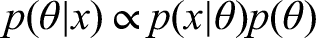
While Bayesian inference incorporates comprehensive statistical methods, its methodological approach originates from Bayes’ theorem:

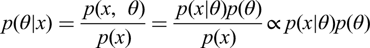
p (θ | x) = \frac{p (x, θ)}{p (x)} = \frac{p (x | θ) p (θ)}{p (x)} \propto p (x | θ) p (θ)

In this theorem, x denotes observed data while $θ$ denotes unobserved parameters. The conditional probability denoted by $p (θ | x)$ represents the probability of the unknown parameters $θ$ given the observed data x. In Bayesian statistics, it is also the posterior probability distribution of $θ$ given x. The denominator $p (x)$ is the prior probability or marginal probability of the observed data x without given conditions. The numerator $p (x, θ)$ is the joint probability distribution of the observed data x and unobserved parameters $θ$ . This joint distribution $p (x, θ)$ can be re-expressed as the product of the conditional probability distribution, $p (x | θ)$ and the marginal probability distribution $p (θ)$ . This conditional distribution represents the probability of the observed data x given the unknown parameters $θ$ and is frequently referred to as the likelihood of the unknown parameters $θ$ given the fixed, known data x. The marginal probability distribution, $p (θ),$ in Bayesian statistics, has been coined as the prior probability distribution of $θ$ , and represents our prior belief about the parameters before the data have been observed. Since $p (x)$ is based on known data and remains constant with different values of the unknown parameters $θ$ , it can be dropped from the equation, resulting in a proportional relation on the right side of the equation $p (θ | x) \propto p (x | θ) p (θ)$ .

Bayes’ theorem constitutes the foundation of modern Bayesian inference. When we interpret statistical probabilities as expressions of our beliefs, the posterior distribution represents our updated beliefs about the unknown parameter $θ$ after building and estimating statistical models with the observed data x. In contrast to dichotomous estimation in NHST (e.g., whether the effect is statistically significant or not), posterior beliefs are understood as distributions (Levy & Mislevy, 2021).

Case Study

We use a case study to illustrate the application of Bayesian statistics in educational leadership and policy studies. Our case study examines the relationship between teachers’ perceptions of school climate and their job satisfaction at U.S. middle schools.

Researchers have demonstrated the significant role of the organizational environment in K-12 activities (Aldridge & Fraser, 2016). Studies have examined the relationship between school climate and teacher job outcomes in different countries, such as Australia (Aldridge & Fraser, 2016), Cameroon (Bahtilla & Hui, 2021), and Norway (Zakariya, 2020). All studies use NHST and report different impact levels of the school climate. Therefore, a Bayesian statistical approach that examines a nationally representative U.S. data set can contribute to our understanding of the relationship between teachers’ perceptions of school climate and their job satisfaction in the U.S.

Data Source

We use data from the Teaching and Learning International Survey (TALIS) 2018. TALIS 2018 is the most recent survey conducted by the Organization for Economic Co-operation and Development (OECD). This survey involved around 260,000 teachers and principals across more than 15,000 schools in 48 countries/economies (OECD, 2019). As the third iteration following TALIS 2008 and TALIS 2013, the 2018 survey was developed using established research design principles, statistical quality checks, and psychometric evaluations (OECD, 2019). TALIS 2018 gathered data on various aspects such as the demographic backgrounds of teachers and principals, their preparedness, and professional outcomes.

This study focuses on the U.S. national data from the TALIS 2018 teacher survey with a sample size of 2560. The OECD conducted psychometric analyses to evaluate the measurement properties of the composite scales. These analyses support the precision of the scores (i.e., reliability) and the appropriateness of score interpretations (i.e., validity) (OECD, 2019). It is, however, important to note that reliability and validity are not fixed test properties. Instead, they are dependent on the sample and context where the test is used (Kane & Burns, 2013; Urbina, 2014).

Variables

To answer our research question, we use the composite scale scores for teachers’ job satisfaction as the response variable, a continuous composite variable based on three subscales: job satisfaction with the work environment, with the profession, and with target class autonomy. The target explanatory variables are three continuous composite scale scores about teachers’ perceptions of school climate. They include: (1) teachers’ perceived disciplinary climate; (2) teacher-student relations; and (3) participation among stakeholders. We also include control variables regarding teachers’ backgrounds and experiences to account for their potential influence. They include: (1) teachers’ gender (categorical: female or male); (2) employment status (categorical: full-time (more than 90% of full-time hours), part-time (71–90%), part-time (50–70%), and part-time (less than 50%)); (3) years of teaching in total (continuous); (4) number of students enrolled in the teacher's class (continuous); and (5) teachers’ self-efficacy (continuous composite variable based on three subscales: self-efficacy in classroom management, in instruction, and in student engagement).

The original questions from TALIS 2018, which were used to develop the selected variables, are detailed in Supplemental Material. The response variable, the teachers’ self-efficacy variable, and the variables about teachers’ perceptions of school climate are composite scale scores constructed from multiple TALIS 2018 questions. The TALIS 2018 technical report (OECD, 2019, pp. 217–430) includes the procedures to construct these scales, including confirmatory factor analysis (CFA) that was conducted separately for each scale using single-factor models with items as indicators. Table 2 in Appendix A presents selected global model fit indices from these CFA models (OECD, 2019), which provide preliminary evidence supporting the internal structure of the scales. It is important to note that global fit indices alone do not establish reliability or validity, and that the categorical nature of the data and local fit indices such as residuals should also be considered when evaluating model adequacy (Appelbaum et al., 2018; Rhemtulla et al., 2012; Stone, 2021).

Methods

Clustered Sampling Design and Bayesian Multilevel Modeling

TALIS 2018 employed a two-stage stratified sampling design to select a representative sample of teachers and schools. In the first stage, schools were sampled using a stratified systematic approach, with probability proportional to their size (number of teachers). Teachers were then randomly sampled within the sampled schools at stage two. An appropriate modeling approach for this hierarchical data structure in which teachers are nested within schools is multilevel modeling or hierarchical linear modeling (Raudenbush & Bryk, 2002). A multilevel model used in the empirical example can be formulated in level notation (Raudenbush & Bryk, 2002) as a system of two equations, one at Level 1, and two at Level 2. The following equations describe the multilevel structure of the model, beginning with the Level 1 (teacher-level) specification and extending to the Level 2 (school-level) formulation:

\begin{matrix} y_{i j} = β_{0 j} + β_{1 j} T 3 D I S C_{i} + β_{2 j} T 3 S T U D_{i} + β_{3 j} T 3 S T A K E_{i} + β_{4 j} T T 3 G 01_{i} + \\ β_{5 j} T T 3 G 10 A_{i} + β_{6 j} T T 3 G 11 B_{i} + β_{7 j} T T 3 G 38_{i} + β_{8 j} T 3 S E L F_{i} + e_{i j}, \end{matrix}

(1)

β_{0 j} = β_{0} + u_{0}

(2a)

β_{1 j} = β_{1} + u_{1}

(2b)

β_{2 j} = β_{2} + u_{2}

(2c)

β_{3 j} = β_{3} + u_{3}

(2d)

β_{4 j} = β_{4}

(2e)

β_{5 j} = β_{5}

(2f)

β_{6 j} = β_{6}

(2g)

β_{7 j} = β_{7}

(2h)

β_{8 j} = β_{8}

(2i)

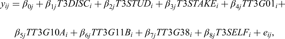
The same multilevel model in matrix notation can be written as,

y_{j} = X_{j} β + Z_{j} u_{j} + e_{j}

(3)

where

y_{j}

is an

n_{j} \times 1

vector of teachers’ job satisfaction scores in school j (

j = 1, \dots, J

X_{j}

is an

n_{j} \times p

design matrix of explanatory variables in school j associated with the p = 8 fixed effects,

β

, and

Z_{j}

is an

n_{j} \times q

design matrix associated with the q = 4 random effects,

u_{j}

. The

n_{j} \times 1

vector of regression errors,

e_{j}

is assumed to be normally distributed with zero mean vector, 0, and diagonal covariance matrix,

Σ

, whose diagonal elements are residual variances,

σ_{e}^{2}

, for each teacher in school j and are assumed to be equal. The random effects are also assumed to follow a normal distribution,

u_{j} \sim N (0, Φ)

, where

Φ = (\begin{matrix} φ_{u_{0}} \\ φ_{u_{1}, u_{0}} & φ_{u_{1}} \\ ⋮ & ⋮ & ⋱ \\ φ_{u_{q}, u_{0}} & φ_{u_{q}, u_{1}} & \dots & φ_{u_{q}} \end{matrix}) .

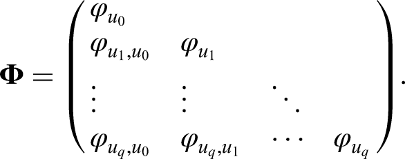
The diagonal elements of $Φ$ are variances of the random effects while the off-diagonal elements are their covariances. In typical applications, the set of q random effects (for random intercepts and slopes) is typically a subset of the p fixed effects, so $q < p$ . It is assumed that $e_{j}$ and $u_{j}$ are uncorrelated.

We implemented the Bayesian multilevel model in R using the rstanarm package (Goodrich et al., 2024), which interfaces with Stan via RStan (Stan Development Team, 2024). Multilevel modeling allows the variation in the response variable to be partitioned into within-school and between-school components. This has two immediate consequences: one statistical and one conceptual. Standard errors associated with fixed effects will be adjusted appropriately based on the hierarchical nature of the data, which will lead to more accurate inferences. Secondly, a model ignoring school-level variability may falsely attribute observed differences in teachers’ job satisfaction scores to individual behaviors without acknowledging that teachers within a school are more alike than what would be expected using a simple random sample. Furthermore, multilevel modeling can be used to understand the impact of explanatory variables at both the teacher and school levels separately and across levels (contextual effects), providing a more comprehensive understanding of the response-predictor(s) relations.

Missing Data and Imputation

TALIS 2018 contains missing data that can affect statistical inference if not addressed properly. We use predictive mean matching (PMM) for data imputation (Little, 1988; Rubin, 1986). PMM predicts the missing values by first building regression models based on the existing data, and then matching each missing value with the observed value that has the closest predicted value. PMM is a semi-parametric method that maximizes the information from the existing data and emphasizes that imputed values are within the realistic range of the observed data. To this end, this approach is different from other methods such as listwise deletion, maximum likelihood estimation (which models missingness directly under specific assumptions), or multiple imputation (which generates multiple data sets to reflect uncertainty). However, it is still important to acknowledge that without access to the true missing values, the accuracy of any imputation remains uncertain.

Weights

Given that the data set is a nationally representative sample, we use statistical methods to address the original stratified design of TALIS 2018 and ensure the findings are nationally representative. The final teacher weight (TCHWGT) is consistently incorporated into the statistical analysis. This means different weights are assigned to teachers based on their representation of the overall population.

In frequentist statistical approaches, the balanced repeated replication (BRR) method is often recommended to accommodate complex survey designs and estimate sampling variability (Jiang, 2021; OECD, 2019). BRR accurately measures variation in results based on sample collection and ensures the reliability of estimates through repeated sampling and calculations (Jiang, 2025; Rao & Shao, 1999).

However, since the robustness of BRR in Bayesian statistics has not been validated (Kaplan & Harra, 2024), we follow current recommendations by normalizing the sampling weights and applying the normalized weights to the data set. The normalization process includes adjusting the weights so that they sum to the sample size. The normalized sampling weights were incorporated directly into the Bayesian estimation through the weights argument in the stan_lmer function, such that each observation contributed to the likelihood proportional to its scaled survey weight. This approach improves convergence of the computing algorithm and helps maintain representativeness while acknowledging the limitations of applying traditional survey weights in Bayesian frameworks.

Prior Distributions

One advantage of Bayesian statistics is the incorporation of prior distributions of model parameters. The choice of a prior distribution in Bayesian inference can depend on different aspects of the data and model such as sample size, parameter type (e.g., regression coefficient, error covariance), and model type (Gelman et al., 2014). As Harring et al. (2017) note, prior distributions in Bayesian inference can be both beneficial and problematic. They allow researchers to incorporate background knowledge into the analysis, which can improve inference. However, inferences can be drawn that are not entirely data-driven if prior distributions are rather informative, if the sample size is modest or small, or the priors are inappropriate or misinformed.

Prior distributions in Bayesian inference can be classified on an “informative” continuum from diffuse (non-informative) to highly informative where the information may come from previous study findings or theoretical predictions. Most distributions used as priors fall into families depending on the kind of parameter to be estimated. For example, it is common to use a normal distribution as a prior for regression coefficients while a gamma or inverse gamma distribution is frequently used for variance components. There are of course multivariate analogs when considering a set of parameters simultaneously. The distribution notwithstanding, characteristics of each distribution include its mean and variance. Prior distributions with large variances are typically referred to as less (non- or weakly) informative than prior distributions with small variances which imply a great deal of information.

For our study, we adopt a decomposable covariance prior with a regularization parameter, a commonly used approach in multilevel models to improve the estimation of covariance structures (Armstrong et al., 2009). As a form of hierarchical prior, it encourages shrinkage in estimates of both correlations and variances of the effects and helps to stabilize estimates in multilevel modeling (Armstrong et al., 2009). Given the limited prior research on this topic within the U.S. context, we intentionally avoided specifying informative priors. Accordingly, no external data or study-specific prior values were included in specifying this prior. We acknowledge that, in the absence of a well-established body of validated research, empirical estimation of prior distribution can introduce risks, such as overfitting or circular reasoning, particularly when prior assumptions are not independently justified (e.g., König & van de Schoot, 2018; Sprenger, 2018). In light of these considerations, this study takes a cautious approach to prior specification to avoid such pitfalls in the multilevel modeling approach:

Fixed effects: $β_{k} \sim N (0, σ_{β}^{2})$ , where $σ_{β}^{2}$ is autoscaled based on the outcome's dispersion. This normal prior provides weak regularization and is centered at zero.

Residual SD: $σ \sim$ Student-t $(v = 3, 0, s_{σ})$ , where $s_{σ}$ is autoscaled. This prior allows for heavier tails and accommodates uncertainty in the residual variance (Gelman et al., 2014).

Random effects: $u_{j} \sim N (0, Σ)$ , where $Σ$ is the covariance matrix of the random effects. We placed a decomposable covariance prior on $Σ$ using decov(regularization = 3), which shrinks correlations among random effects toward zero and regularizes the variance components (Gelman et al., 2014).

We specified the priors to regularize estimation while allowing the data to remain the primary driver of inference. Specifically, these priors were selected to stabilize estimation in the multilevel context without imposing strong substantive assumptions. We examined model estimates under alternative reasonable prior scales and observed no substantive changes in the results, suggesting that findings were not sensitive to prior specification.

Posterior Distributions and Credible Intervals

A central goal of Bayesian inference is to obtain the posterior distributions of parameters from which inferences are drawn. According to Bayes’ Theorem, the posterior distribution of parameters, $θ$ , given the observed data is proportional to the likelihood of the data given these parameters multiplied by the prior distribution of $θ$ , and is expressed as:

p (θ | x) \propto p (x | θ) p (θ)

The fact that the result of a Bayesian analysis is a distribution implies that its characteristics can be expressed using graphical summaries such as histograms or density plots as well as numerical summaries such as measures of central tendency (i.e., median or mean) and variability (i.e., standard deviation). As Levy and Mislevy (2017, 2021), among others, have emphasized, the posterior distribution can also be summarized with an interval indicating the region that delineates a given percentage of the distribution, referred to as a credible interval.

The Bayesian construction of credible intervals contributes to estimation thinking (Gelman et al., 2014). Credible intervals describe the uncertainty related to the unknown parameters using a probability distribution, the posterior distribution, which represents all knowledge and evidence about the population distribution at the moment. It is important to note the differences between Bayesian credible intervals and frequentist confidence intervals. The frequentist approach uses a confidence interval to offer a range of values that is likely to encompass the true population parameter with a specified probability. To this end, the probability that the interval contains the target parameter is either 0 or 1. In contrast, Bayesian inference uses a credible interval to represent the probability that a parameter lies within a specified range. For instance, a 95% credible interval denotes that the probability that the value of the parameter lies within this range is 0.95.

Compared to the frequentist approach, the credible interval not only offers a more intuitive interpretation that aligns better with our common sense but also supports estimation thinking that transcends dichotomous reporting and conclusions. For example, a frequentist confidence interval that contains the value of 0 is widely reported as statistically insignificant in many applied quantitative studies without further investigating its effect size. In contrast, even if a Bayesian credible interval contains the value of zero, the distribution of credible values may show a significant difference between zero and the observed effect, which could be substantively important. This is especially relevant when evaluating how much the estimated effect differs from zero.

MCMC Algorithms

Estimating parameters within Bayesian statistics is typically carried out using Markov chain Monte Carlo (MCMC) methods such as Gibbs sampling, the random-walk Metropolis-Hastings algorithm, or the No-U-Turn sampler, an extension of the Hamiltonian Monte Carlo algorithm. MCMC methods finesse sampling directly from the joint posterior distribution, which is difficult to sample from, by sampling from the full conditional posteriors of each parameter conditioned on the data and the most recent value of all other parameters (e.g., Gelman et al., 2014; Levy et al., 2011). For our study, we sampled from the posterior using Stan's No-U-Turn Sampler.

Convergence

An important task in Bayesian analysis is assessing the convergence of the MCMC algorithm to the posterior distribution of the parameters. MCMC is an iterative process where values of each parameter (called chains) are estimated from several successive draws from the posterior distribution. Although no standard exists in the literature, conventional wisdom suggests that any MCMC algorithm starts from at least two (if not more) initial values of the parameters creating multiple chains. Monitoring the values of these chains through trace plots ensures the convergence of the iteration process to a stationary estimate of the posterior distributions. Convergence can be evaluated by calculating the potential scale reduction factor (PSRF, or R̂; Brooks & Gelman, 1998; Kaplan & Harra, 2024). Analogous to an ANOVA decomposition, the PSRF is computed as the ratio of total variance (the sum of between-chains and within-chain variance) across chains to the pooled variance within chains. Once this ratio reflects very little variance between chains when compared to within-chain variance (i.e., PSRF < 1.05) for each model parameter, estimation is halted, and convergence is claimed. The Kolmogorov-Smirnov test to assess the equivalence of posterior distributions across chains can be used in addition to the PSRF to assess convergence (Brooks et al., 2003). Effective sample size (ESS) is another convergence diagnostic and quantifies the amount of independent information present in the correlated samples inherent with all MCMC algorithms. ESS adjusts the raw sample size by taking into account the autocorrelation structure in the MCMC draws.

Posterior Predictive Checking

Bayesian inference often uses posterior predictive model checking (PPMC) to assess how well a model fits the actual data (Gelman et al., 2014). The PPMC method involves comparing the actual observed data x to data simulated from the model's posterior predictive distribution, xrep, to see if the observed outcomes are unusually extreme. A discrepancy measure, $D (x, θ),$ is defined and the posterior distribution of $D (x, θ)$ is compared to the posterior predictive distribution $D (x r e p, θ)$ with a substantial difference between them indicating model misfit. Although graphical plots can be used to compare observed and replicated discrepancy measures, a tail-area probability known as the posterior predictive probability (PPP)-value is often used instead. The PPP-values provide a quantitative measure of the degree to which observed data, such as the data in the sample, would be expected under the model. In this study, we used the sample mean as the discrepancy measure in posterior predictive checking. Specifically, for each replicated data set, the mean of the outcome variable was computed and compared to the observed mean, and the PPP-value was calculated as the proportion of replicated data sets in which this statistic exceeded the observed value. This provides a diagnostic of how well the model reproduces this key feature of the observed data. PPP-values representing extremely small probabilities (i.e., less than 0.05 or greater than 0.95) are very suggestive that the model does not capture the corresponding feature of the data while PPP-values close to 0.5 indicate that there are no systematic differences between the realized and predictive values, and thus an adequate fit of the model (Sinharay, 2006).

Results and Findings

In this section, we report the results of the Bayesian multilevel model. The model includes both teacher-level and school-level predictors, and estimates were obtained using MCMC methods. Following Kaplan and Harra's (2024) recommendation on MCMC, we ran the model using four separate chains, each with 5,000 iterations. The first half of these iterations (2,500) were used for burn-in samples, which helps the algorithm stabilize as it finds its way to the posterior distribution. We then applied a thinning interval of 10, meaning we only kept every 10th iteration from the remaining 2,500 iterations. This process resulted in a total of 1,000 iterations (250 iterations per chain) being used for our final analysis.

Model Fit and Convergence

Figure 1 presents the posterior predictive checking results. A PPP-value close to 0.5 indicates that the model-generated data closely resemble the observed data, whereas values near 0 or 1 suggest a poor fit. The PPP-value is 0.568, suggesting that the model-generated data are reasonably consistent with the observed data based on the chosen discrepancy measure (Gelman et al., 2014). To complement PPP, we also computed the Watanabe-Akaike Information Criterion (WAIC) using the loo package in R (Vehtari et al., 2017; Vehtari et al., 2024). WAIC provides an estimate of out-of-sample predictive accuracy, with lower values indicating better expected predictive performance. WAIC is reported to enhance transparency regarding model adequacy. The WAIC value was 11,357.6 (SE = 357.8), with an estimated effective number of parameters (p_waic) of 83.3 (SE = 16.6). Although 1.0% of p_waic estimates exceeded 0.4, the WAIC remains a reasonable indicator of model fit.

Figure 1.

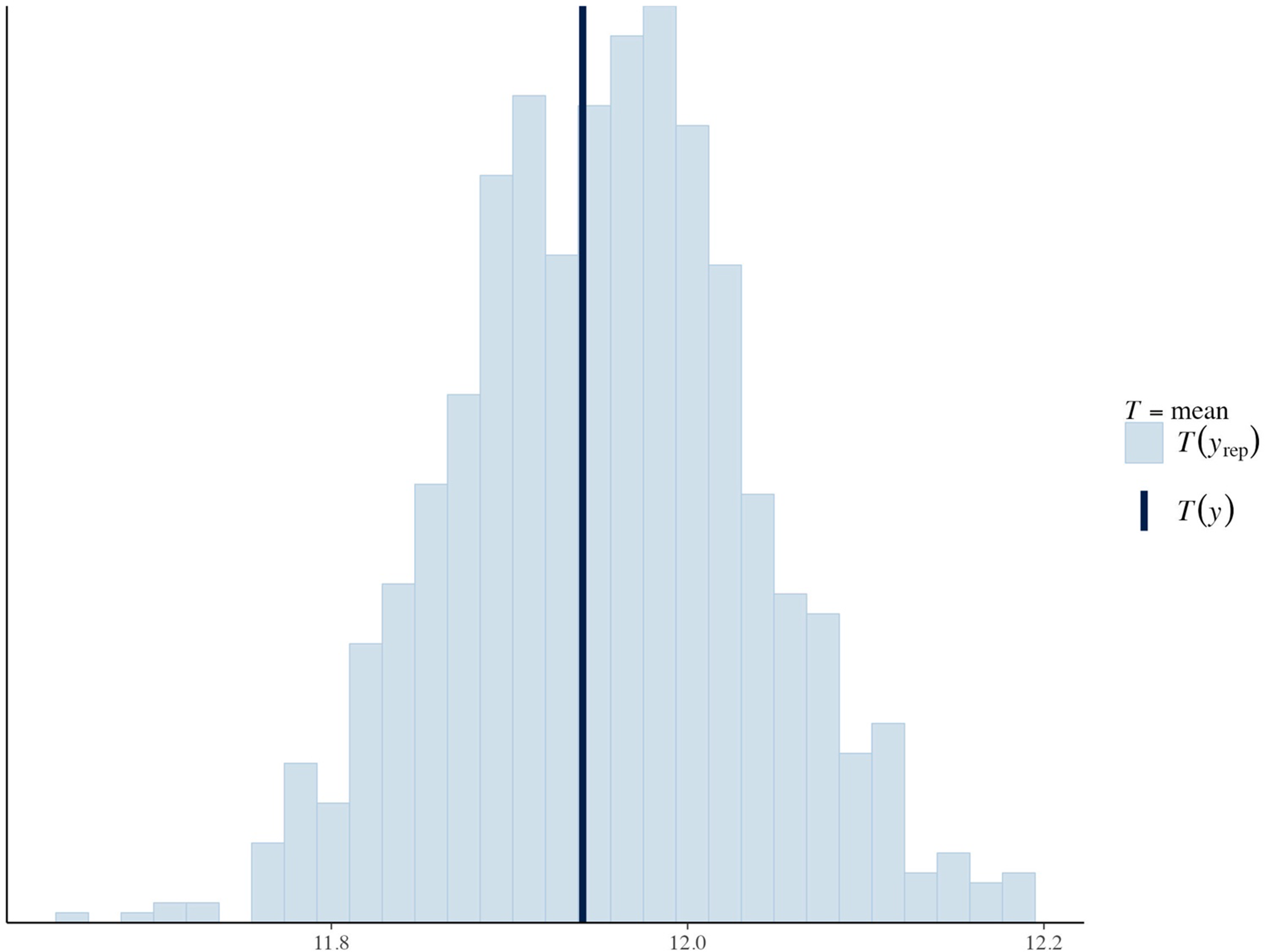
Posterior predictive checking plot (PPP-value = 0.568).

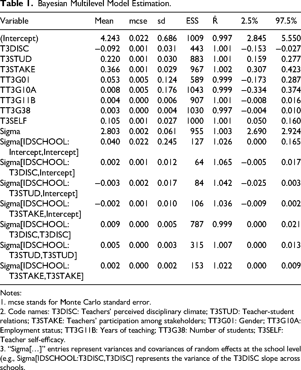
The convergence diagnostics in Table 1 show that the PSRF (R̂) values are close to 1 and the ESS are sufficiently large for most parameters, indicating that the MCMC chains have converged and the posterior estimates are stable. In addition to R̂ and ESS, we also visually inspected trace plots to confirm convergence.

Table 1.

Bayesian Multilevel Model Estimation.

Variable	Mean	mcse	sd	ESS	R̂	2.5%	97.5%
(Intercept)	4.243	0.022	0.686	1009	0.997	2.845	5.550
T3DISC	−0.092	0.001	0.031	443	1.001	−0.153	−0.027
T3STUD	0.220	0.001	0.030	883	1.001	0.159	0.277
T3STAKE	0.366	0.001	0.029	967	1.002	0.307	0.423
TT3G01	0.053	0.005	0.124	589	0.999	−0.173	0.287
TT3G10A	0.008	0.005	0.176	1043	0.999	−0.334	0.374
TT3G11B	0.004	0.000	0.006	907	1.001	−0.008	0.016
TT3G38	0.003	0.000	0.004	1030	0.997	−0.004	0.010
T3SELF	0.105	0.001	0.027	1000	1.001	0.050	0.160
Sigma	2.803	0.002	0.061	955	1.003	2.690	2.924
Sigma[IDSCHOOL:Intercept,Intercept]	0.040	0.022	0.245	127	1.026	0.000	0.165
Sigma[IDSCHOOL:T3DISC,Intercept]	0.002	0.001	0.012	64	1.065	−0.005	0.017
Sigma[IDSCHOOL:T3STUD,Intercept]	−0.003	0.002	0.017	84	1.042	−0.025	0.003
Sigma[IDSCHOOL:T3STAKE,Intercept]	−0.002	0.001	0.010	106	1.036	−0.009	0.002
Sigma[IDSCHOOL:T3DISC,T3DISC]	0.009	0.000	0.005	787	0.999	0.000	0.021
Sigma[IDSCHOOL:T3STUD,T3STUD]	0.005	0.000	0.003	315	1.007	0.000	0.013
Sigma[IDSCHOOL:T3STAKE,T3STAKE]	0.002	0.000	0.002	153	1.022	0.000	0.009

Notes:

1. mcse stands for Monte Carlo standard error.

2. Code names: T3DISC: Teachers’ perceived disciplinary climate; T3STUD: Teacher-student relations; T3STAKE: Teachers’ participation among stakeholders; TT3G01: Gender; TT3G10A: Employment status; TT3G11B: Years of teaching; TT3G38: Number of students; T3SELF: Teacher self-efficacy.

3. “Sigma[…]” entries represent variances and covariances of random effects at the school level (e.g., Sigma[IDSCHOOL:T3DISC,T3DISC] represents the variance of the T3DISC slope across schools.

Key Findings

We use Table 1 to interpret the estimated model that investigates the factors influencing teacher job satisfaction. The intercept of the model is estimated at 4.243 (95% Credible Interval (CrI): [2.845, 5.550]), indicating the baseline level of teacher job satisfaction when all other predictors are at their reference levels. The coefficient for the variable of teachers’ perceived disciplinary climate is −0.092 (95% CrI: [-0.153, −0.027]). As a larger value denotes a more negative perception of the disciplinary climate (see Supplemental Material for details), this coefficient implies that a better disciplinary climate is associated with higher job satisfaction. This suggests a more favorable disciplinary climate in schools is associated with higher levels of teachers’ job satisfaction. Next, the coefficient for the variable of teacher-student relations is 0.220 (95% CrI: [0.159, 0.277]), demonstrating its positive association with job satisfaction. Better teacher-student relations are linked to higher job satisfaction. Furthermore, the coefficient for the variable of teachers’ participation among stakeholders is 0.366 (95% CrI: [0.307, 0.423]), indicating its strong positive association with job satisfaction as well. Among these three explanatory variables, teachers’ participation among stakeholders has the largest effect size on their job satisfaction, followed by their relations with students and perception of disciplinary climate.

Table 1 also reports the results for the control variables. The coefficient for gender is 0.053 (95% CrI: [-0.173, 0.287]). This result shows a minimal effect with a wide credible interval, suggesting uncertainty in the estimate. The coefficient for current employment status is 0.008 (95% CrI: [-0.334, 0.374]), showing a negligible effect on job satisfaction. The coefficient for years of teaching is 0.004 (95% CrI: [-0.008, 0.016]), indicating a very small effect as well. The coefficient for the number of students is 0.003 (95% CrI: [-0.004, 0.010]), showing minimal impact on job satisfaction. The coefficient for teacher self-efficacy is 0.105 (95% CrI: [0.050, 0.160]), indicating a positive association. Higher self-efficacy is linked to greater job satisfaction. Sigma, or the residual standard deviation is estimated at 2.803 (95% CrI: [2.690, 2.924]), indicating the variability in job satisfaction not explained by the model.

For this estimated multilevel model, the variances and covariances of the intercepts and variables across schools provide insights into how they vary at the school level. For example, the covariance parameter Sigma[IDSCHOOL:T3DISC, Intercept] represents the extent to which schools with higher baseline job satisfaction (intercepts) tend to differ in the effect of disciplinary climate on job satisfaction. In our model, the estimated covariance is 0.002 (95% CrI: [-0.005, 0.017]), which is close to zero, suggesting little systematic relations between schools’ average job satisfaction and the strength of the disciplinary climate effect. In practical terms, this means that schools with higher or lower baseline satisfaction do not consistently show stronger or weaker associations between disciplinary climate and job satisfaction. Similarly, the other covariance estimates (e.g., between intercepts and T3STUD or T3STAKE slopes) are also close to zero. Likewise, the small variance estimates for these slopes indicate that the strength of these relations is fairly consistent across schools, with limited between-school heterogeneity. In practical terms, this means that the impact of disciplinary climate, teacher-student relations, and stakeholder participation on job satisfaction is fairly consistent across schools, with little evidence of strong school-level moderation. The relatively small between-school variance suggests that differences in teacher job satisfaction are driven more by individual-level perceptions than by structural differences across schools. This has implications for educational leadership practice, indicating that interventions targeting school climate may also need to focus on within-school processes (e.g., teacher-student relations and stakeholder participation) rather than relying solely on school-level structural reforms.

To compare the Bayesian approach with the frequentist approach, we also analyzed the same data with the maximum likelihood estimation using a quasi-Newton optimization routine and robust standard errors. The results of the estimated model are provided in Table 3 in Appendix B. Relative to the frequentist multilevel results, the Bayesian analysis provides full posterior distributions and 95% credible intervals for each parameter, enabling direct probability statements (e.g., the probability that an effect exceeds zero). Signs and rank-ordering of key climate effects are consistent across frameworks, but Bayesian intervals for variance components avoid implausible negative bounds and better respect parameter constraints. Posterior predictive checking complements WAIC, providing model-based evidence that the fitted model reproduces salient features of the outcome distribution. These features illustrate the practical advantages of Bayesian methods for multilevel modeling in complex survey data. Therefore, this comparison underscores the benefits of Bayesian inference: (1) coherent interval estimates that respect parameter constraints, (2) the ability to incorporate prior information, and (3) richer interpretation through posterior distributions. These advantages are particularly relevant for educational research using hierarchical data, where variance components and small-sample uncertainty are critical.

The findings in this case study provide practical implications for educational administration. First, schools may consider initiatives to enhance the disciplinary climate, as this factor is associated with higher levels of job satisfaction among teachers. Second, encouraging and fostering positive interactions between teachers and students can be linked to higher levels of job satisfaction among teachers. Third, schools may benefit from creating more opportunities for stakeholder involvement, which is related to higher job satisfaction among teachers. Furthermore, providing professional development opportunities that enhance teachers’ self-efficacy can be linked to higher job satisfaction among teachers as well.

In summary, we use the case study as a step-by-step example to illustrate how Bayesian statistics can be implemented in educational leadership and policy studies. This illustration provides readers with both a theoretical interpretation and a practical implementation of Bayesian statistics to complex, stratified survey data in education. The illustration also demonstrates the advantages of using Bayesian statistics in educational leadership and policy studies compared to traditional frequentist inferences. For example, Bayesian approaches allow the incorporation of past research to update our knowledge with new data, contributing to the accumulation of knowledge. Also, instead of using NHST that easily falls within the dichotomous thinking of reporting a p-value (Wasserstein et al., 2019), Bayesian approaches support the direct estimation of uncertainty about our beliefs (parameters). For instance, by reporting the results from Table 1, the analysis demonstrates a key benefit of using Bayesian methods for analyzing and reporting educational data: the ability to look at the entire posterior distribution of the effect. Compared to frequentist inference, this is particularly helpful when the NHST approach leads to a p-value larger than the threshold (or a confidence interval that contains zero) and a conclusion of statistical non-significance is then assumed. Furthermore, statistical diagnostics in Bayesian inferences, such as posterior predictive checks, also promote the robustness and power of the selected model. If prior knowledge influences the choice of prior distributions, it's standard practice to conduct a sensitivity analysis. This helps assess how much the results depend on those priors. Differences in outcomes under alternative priors are typically evaluated using model comparison metrics, such as WAIC or DIC (Deviance Information Criterion).

A Heuristic for Implementing Bayesian Inference

Based on our analysis, we provide a heuristic for implementing Bayesian inference in educational leadership and policy studies.

Identify the research problem and define research questions: Like most quantitative studies, clearly state the educational problem and propose research questions that guide the study.

Collect data: Obtain data from educational surveys, experiments, and/or evaluations. Data can come from different sources. For example, they can be primary data collected specifically to answer the research questions. They can also be secondary data sets from large-scale surveys, such as the one used in this case study.

Specify the statistical model: Select a Bayesian model that aligns with the characteristics of the data and fits the research design and questions. This could range from a simple linear regression model to a more complex model, such as the multilevel model used in this study.

Select distributions for priors of parameters: Choose prior distributions based on existing knowledge. The priors can be informative, weakly informative, or non-informative. If relevant, the informative or weakly informative priors should address previous research on the chosen topic.

Calculate the posterior: Apply Bayesian methods to update the prior distributions with the collected data and obtain posterior distributions. This analytical procedure often incorporates computational techniques such as MCMC.

Assess convergence and model diagnostics: Examine convergence diagnostics (e.g., trace plots, R̂, ESS, and autocorrelation) to ensure reliable posterior estimation. If necessary, adjust model specifications or sampling parameters and rerun the analysis.

Interpret results: Analyze and assess the posterior distributions to draw conclusions about the research question. In addition to the means, other statistics representing the posterior distributions, such as credible intervals, should also be reported.

Report and communicate: Present the findings in a clear and accessible manner, highlighting the probabilistic nature of the results and their implications for educational leadership and policy.

Iterate and refine: Consistently refine the model and approach based on feedback and new data. Use the posterior distributions as priors for future research so they can be updated with new posterior distributions.

Conclusions and Implications

In this paper, we present and apply Bayesian statistics within the realm of educational leadership and policy studies. We examine the conceptual and statistical foundations, provide practical illustrations, and offer a heuristic for implementing Bayesian methods in the field. By applying Bayesian techniques, we aim to enhance the quality, validity, and reliability of quantitative research in educational leadership and policy, thereby increasing the impact and applicability of these scholarly efforts. The Bayesian framework used in this study supports an estimation-focused approach by emphasizing the magnitude and uncertainty of effects rather than binary decision-making based on statistical significance. This perspective also aligns with recent calls for estimation thinking in educational leadership and policy research (Xia, 2024).

This paper offers guidance for quantitative researchers in educational leadership and policy on incorporating Bayesian statistics as a robust and informative approach in their work (Gelman et al., 2014). Beyond the case study presented, researchers can apply Bayesian methods to various data and topics, such as program evaluation, school administrator ratings, teacher assessment, and student performance. Additionally, similar Bayesian approaches can be utilized to analyze other complex survey data sets, such as the National Assessment of Educational Progress (NAEP), National Teacher and Principal Survey (NTPS), High School Longitudinal Study of 2009 (HSLS: 09), and state-level assessment data.

Supplemental Material

sj-odt-1-eaq-10.1177_0013161X261461704 - Supplemental material for Leveraging Bayesian Statistics in Educational Leadership and Policy Studies

Supplemental material, sj-odt-1-eaq-10.1177_0013161X261461704 for Leveraging Bayesian Statistics in Educational Leadership and Policy Studies by Lei Jiang and Jeffrey R. Harring in Educational Administration Quarterly

Footnotes

ORCID iD

Lei Jiang

Funding

The authors disclosed receipt of the following financial support for the research, authorship, and/or publication of this article: This work was supported in part by research funding from the University of Kansas Office of Research.

Declaration of Conflicting Interests

The authors declared no potential conflicts of interest with respect to the research, authorship, and/or publication of this article.

Supplemental Material

Supplemental material for this article is available online.

Author Biographies

Lei Jiang is an Assistant Professor in the Department of Educational Leadership and Policy Studies at the University of Kansas. His research focuses on educational leadership and policy, multilingual education, and research methodologies, including quantitative methods. He holds a Ph.D. in Education and an M.S. in Statistics from the University of Georgia, and an M.Ed. from Harvard University. He has recently published in journals such as Educational Policy, Educational Administration Quarterly, TESOL Quarterly, among others.

Jeffrey R. Harring is a Professor in the Department of Human Development and Quantitative Methodology at the University of Maryland. He holds a Ph.D. in Educational Psychology from the University of Minnesota. His recent work has appeared in journals such as Structural Equation Modeling: A Multidisciplinary Journal, Educational and Psychological Measurement, and Reading and Writing.

Appendix A

Table 2.

CFA Model-Data Fit for the Selected Composite Scales or Subscales.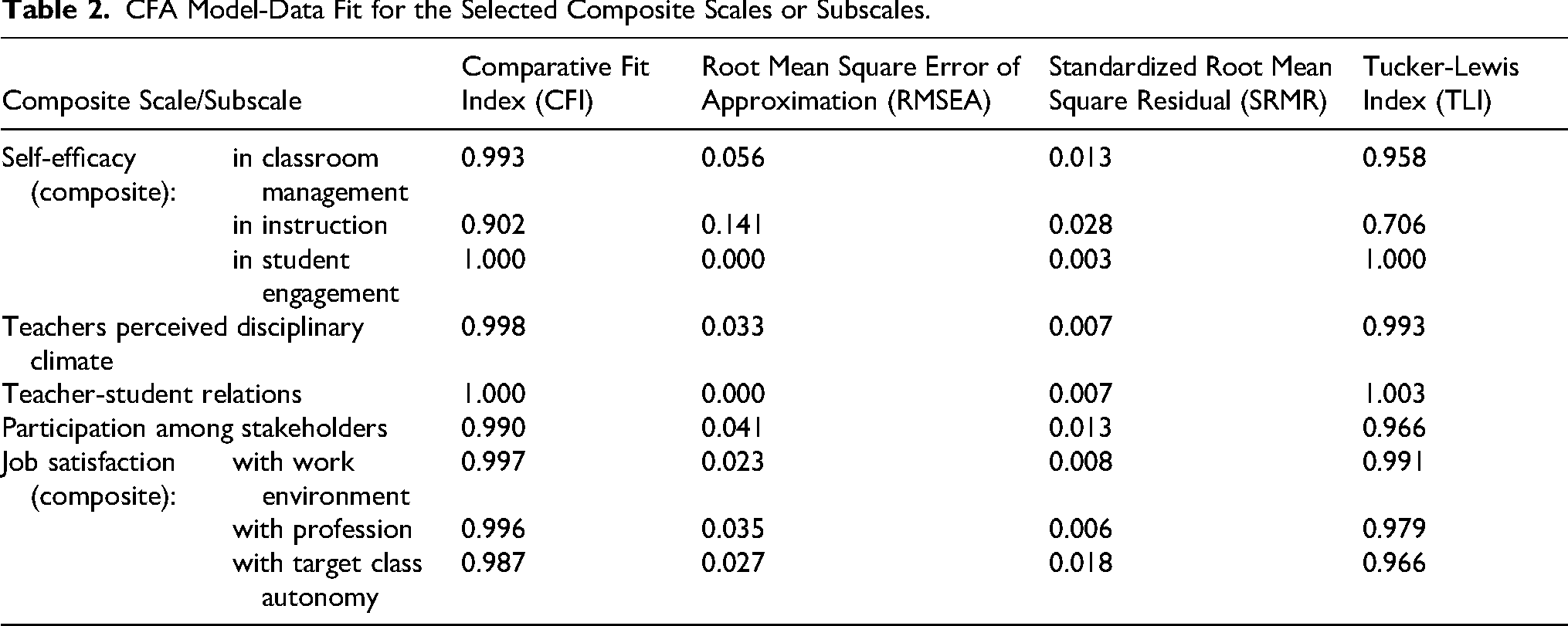

Composite Scale/Subscale		Comparative Fit Index (CFI)	Root Mean Square Error of Approximation (RMSEA)	Standardized Root Mean Square Residual (SRMR)	Tucker-Lewis Index (TLI)
Self-efficacy (composite):	in classroom management	0.993	0.056	0.013	0.958
	in instruction	0.902	0.141	0.028	0.706
	in student engagement	1.000	0.000	0.003	1.000
Teachers perceived disciplinary climate		0.998	0.033	0.007	0.993
Teacher-student relations		1.000	0.000	0.007	1.003
Participation among stakeholders		0.990	0.041	0.013	0.966
Job satisfaction (composite):	with work environment	0.997	0.023	0.008	0.991
	with profession	0.996	0.035	0.006	0.979
	with target class autonomy	0.987	0.027	0.018	0.966

Appendix B

Table 3.

Frequentist Multilevel Model (MLR): Estimates, SEs, P-values, and Wald 95% Cis.

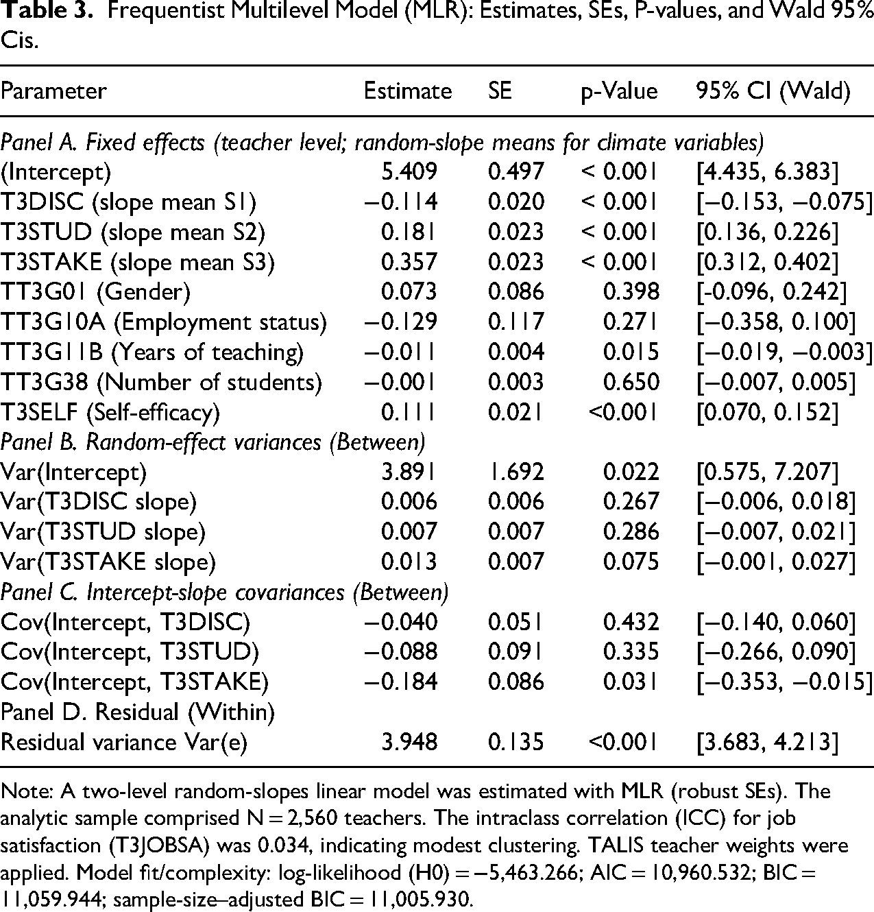
Parameter	Estimate	SE	p-Value	95% CI (Wald)
Panel A. Fixed effects (teacher level; random-slope means for climate variables)
(Intercept)	5.409	0.497	< 0.001	[4.435, 6.383]
T3DISC (slope mean S1)	−0.114	0.020	< 0.001	[−0.153, −0.075]
T3STUD (slope mean S2)	0.181	0.023	< 0.001	[0.136, 0.226]
T3STAKE (slope mean S3)	0.357	0.023	< 0.001	[0.312, 0.402]
TT3G01 (Gender)	0.073	0.086	0.398	[-0.096, 0.242]
TT3G10A (Employment status)	−0.129	0.117	0.271	[−0.358, 0.100]
TT3G11B (Years of teaching)	−0.011	0.004	0.015	[−0.019, −0.003]
TT3G38 (Number of students)	−0.001	0.003	0.650	[−0.007, 0.005]
T3SELF (Self-efficacy)	0.111	0.021	<0.001	[0.070, 0.152]
Panel B. Random-effect variances (Between)
Var(Intercept)	3.891	1.692	0.022	[0.575, 7.207]
Var(T3DISC slope)	0.006	0.006	0.267	[−0.006, 0.018]
Var(T3STUD slope)	0.007	0.007	0.286	[−0.007, 0.021]
Var(T3STAKE slope)	0.013	0.007	0.075	[−0.001, 0.027]
Panel C. Intercept-slope covariances (Between)
Cov(Intercept, T3DISC)	−0.040	0.051	0.432	[−0.140, 0.060]
Cov(Intercept, T3STUD)	−0.088	0.091	0.335	[−0.266, 0.090]
Cov(Intercept, T3STAKE)	−0.184	0.086	0.031	[−0.353, −0.015]
Panel D. Residual (Within)
Residual variance Var(e)	3.948	0.135	<0.001	[3.683, 4.213]

Note: A two-level random-slopes linear model was estimated with MLR (robust SEs). The analytic sample comprised N = 2,560 teachers. The intraclass correlation (ICC) for job satisfaction (T3JOBSA) was 0.034, indicating modest clustering. TALIS teacher weights were applied. Model fit/complexity: log-likelihood (H0) = −5,463.266; AIC = 10,960.532; BIC = 11,059.944; sample-size–adjusted BIC = 11,005.930.

References

(2016). Teachers’ views of their school climate and its relationship with teacher self-efficacy and job satisfaction. Learning Environments Research, 19(2), 291–307. https://doi.org/10.1007/s10984-015-9198-x

Appelbaum

Cooper

Kline

R. B.

Mayo-Wilson

Nezu

A. M.

Rao

S. M.

(2018). Journal article reporting standards for quantitative research in psychology: The APA publications and communications board task force report. American Psychologist, 73(1), 3–25. https://doi.org/10.1037/amp0000191

Armstrong

Carter

C. K.

Wong

K. F. K.

Kohn

(2009). Bayesian Covariance matrix estimation using a mixture of decomposable graphical models. Statistics and Computing, 19(3), 303–316. https://doi.org/10.1007/s11222-008-9093-8

Bahtilla

Hui

(2021). The impact of school environment on teachers’ job satisfaction in secondary schools. European Journal of Education Studies, 8(7), 16–43. https://doi.org/10.46827/ejes.v8i7.3799

Brooks

S. P.

Gelman

(1998). General methods for monitoring convergence of iterative simulations. Journal of Computational and Graphical Statistics, 7(4), 434–455. https://doi.org/10.1080/10618600.1998.10474787

Brooks

S. P.

Giudici

Philippe

(2003). Nonparametric convergence assessment for MCMC model selection. Journal of Computational and Graphical Statistics, 12, 1–22. https://doi.org/10.1198/1061860031347

Cohen

(1994). The earth is round (p<.05). American Psychologist, 49(12), 997–1003. https://doi.org/10.1037/0003-066X.49.12.997

Cumming

(2014). The new statistics: Why and how. Psychological Science, 25(1), 7–29. https://doi.org/10.1177/0956797613504966

Fan

(2001). Statistical significance and effect size in education research: Two sides of a coin. The Journal of Educational Research, 94(5), 275–282. https://doi.org/10.1080/00220670109598763

10.

Fox

J.-P.

(2010). Bayesian item response modeling: Theory and applications. Springer.

11.

Gelman

Carlin

J. B.

Stern

H. S.

Dunson

D. B.

Vehtari

Rubin

D. B.

(2014). Bayesian data analysis. Chapman and Hall/CRC. https://doi.org/10.1201/b16018

12.

Gill

(2015). Bayesian methods: A social and behavioral sciences approach. Chapman and Hall/CRC. https://doi.org/10.1201/9781420057478

13.

Goodrich

Gabry

Ali

Brilleman

(2024). rstanarm: Bayesian applied regression modeling via Stan. R package version 2.32.1. https://mc-stan.org/rstanarm

14.

Harring

J. R.

McNeish

Hancock

G. R.

(2017). Using phantom variables in structural equation modeling to assess model sensitivity to external misspecification. Psychological Methods, 22(4), 616–631. https://doi.org/10.1037/met0000103

15.

Jiang

(2021). English learner students and college access in the U.S.: Analyzing thirty years of evidence from the National Secondary School Longitudinal Studies (Publication No. 28548531) [Doctoral dissertation]. University of Georgia. ProQuest Dissertation and Theses Global.

16.

Jiang

(2025). Multicultural/multilingual preparation and professional outcomes: Exploring self-efficacy, instructional practices, and job satisfaction among STEM teachers of multilingual learners. Journal of Multilingual and Multicultural Development, 1–18. https://doi.org/10.1080/01434632.2025.2598442

17.

Kane

Burns

(2013). The argument-based approach to validation. School Psychology Review, 42(4), 448–457. https://doi.org/10.1080/02796015.2013.12087465

18.

Kaplan

(2023). Bayesian statistics for the social sciences. Guilford Press.

19.

Kaplan

Harra

(2024). A Bayesian workflow for the analysis and reporting of international large-scale surveys: A case study using the OECD teaching and learning international survey. Large-scale Assessments in Education, 12(2), 1–36. https://doi.org/10.1186/s40536-023-00189-1

20.

König

van de Schoot

(2018). Bayesian Statistics in educational research: A look at the current state of affairs. Educational Review, 70(4), 486–509. https://doi.org/10.1080/00131911.2017.1350636

21.

Levy

Mislevy

R. J.

(2017). Bayesian psychometric modeling. Chapman and Hall/CRC. https://doi.org/10.1201/9781315374604

22.

Levy

Mislevy

R. J.

(2021). A history of Bayesian inference in educational measurement. In Clauser

B. E.

Bunch

M. B.

(Eds.), The history of educational measurement (pp. 292–317). Routledge.

23.

Levy

Mislevy

R. J.

Behrens

J. T.

(2011). MCMC In educational research. In Brooks

Gelman

Jones

G. L.

Meng

X.-L.

(Eds.), Handbook of Markov chain Monte Carlo (pp. 531–545). Chapman and Hall/CRC.

24.

Little

R. J.

(1988). Missing-data adjustments in large surveys. Journal of Business & Economic Statistics, 6(3), 287–296. https://doi.org/10.2307/1391878

25.

Organization for Economic Cooperation and Development. (2019). TALIS 2018 technical report. OECD Publishing, https://www.oecd.org/education/talis/TALIS_2018_Technical_Report.pdf .

26.

Rao

J. N. K.

Shao

(1999). Modified balanced repeated replication for complex survey data. Biometrika, 86(2), 403–415. https://doi.org/10.1093/biomet/86.2.403

27.

Raudenbush

S. W.

Bryk

A. S.

(2002). Hierarchical linear models: Applications and data analysis methods. Sage.

28.

Rhemtulla

Brosseau-Liard

P. É.

Savalei

(2012). When can categorical variables be treated as continuous? A comparison of robust continuous and categorical SEM estimation methods under suboptimal conditions. Psychological Methods, 17(3), 354–373. https://doi.org/10.1037/a0029315

29.

Rubin

D. B.

(1986). Statistical matching using file concatenation with adjusted weights and multiple imputations. Journal of Business & Economic Statistics, 4(1), 87–94. https://doi.org/10.2307/1391390

30.

Sinharay

(2006). Model diagnostics for Bayesian networks. Journal of Educational and Behavioral Statistics, 31(1), 1–33. https://doi.org/10.3102/10769986031001001

31.

Sprenger

(2018). The objectivity of subjective Bayesianism. European Journal for Philosophy of Science, 8(3), 539–558. https://doi.org/10.1007/s13194-018-0200-1

32.

Stan Development Team. (2024). RStan: the R interface to Stan. R package version 2.32.6. https://mc-stan.org/

33.

Stone

B. M.

(2021). The ethical use of fit indices in structural equation modeling: Recommendations for psychologists. Frontiers in Psychology, 12, 1–4. https://doi.org/10.3389/fpsyg.2021.783226

34.

Thum

Y. M.

Bhattacharya

S. K.

(2001). Detecting a change in school performance: A Bayesian analysis for a multilevel join point problem. Journal of Educational and Behavioral Statistics, 26(4), 443–468. https://doi.org/10.3102/10769986026004443

35.

Urbina

(2014). Essentials of psychological testing (2nd ed.). Wiley.

36.

Vehtari

Gabry

Magnusson

Yao

Bürkner

Paananen

Gelman

(2024). loo: Efficient leave-one-out cross-validation and WAIC for Bayesian models. R package version 2.7.0. <https://mc-stan.org/loo/>

37.

Vehtari

Gelman

Gabry

(2017). Practical Bayesian model evaluation using leave-one-out cross-validation and WAIC. Statistics and Computing, 27(5), 1413–1432. https://doi.org/10.1007/s11222-016-9696-4

38.

Wasserstein

R. L.

Lazar

N. A.

(2016). The ASA statement on p-values: Context, process, and purpose. The American Statistician, 70(2), 129–133. https://doi.org/10.1080/00031305.2016.1154108

39.

Wasserstein

R. L.

Schirm

A. L.

Lazar

N. A.

(2019). Moving to a world beyond “p< 0.05”. The American Statistician, 73(sup1), 1–19. https://doi.org/10.1080/00031305.2019.1583913

40.

Xia

(2024). A paradigm shift to estimation thinking in quantitative research in educational leadership. Educational Administration Quarterly, 60(2), 269–271. https://doi.org/10.1177/0013161X241242599

41.

Zakariya

Y. F.

(2020). Effects of school climate and teacher self-efficacy on job satisfaction of mostly STEM teachers: A structural multigroup invariance approach. International Journal of STEM Education, 7, 1–12. https://doi.org/10.1186/s40594-020-00209-4

Supplementary Material

Please find the following supplemental material available below.

For Open Access articles published under a Creative Commons License, all supplemental material carries the same license as the article it is associated with.

For non-Open Access articles published, all supplemental material carries a non-exclusive license, and permission requests for re-use of supplemental material or any part of supplemental material shall be sent directly to the copyright owner as specified in the copyright notice associated with the article.

0.03 MB

0.00 MB