






Abstract
The one-parameter logistic model with ability-based guessing (1PL-AG) has been recently developed to account for effect of ability on guessing behavior in multiple-choice items. In this study, the authors developed algorithms for computerized classification testing under the 1PL-AG and conducted a series of simulations to evaluate their performances. Four item selection methods (the Fisher information, the Fisher information with a posterior distribution, the progressive method, and the adjusted progressive method) and two termination criteria (the ability confidence interval [ACI] method and the sequential probability ratio test [SPRT]) were developed. In addition, the Sympson–Hetter online method with freeze (SHOF) was implemented for item exposure control. Major results include the following: (a) when no item exposure control was made, all the four item selection methods yielded very similar correct classification rates, but the Fisher information method had the worst item bank usage and the highest item exposure rate; (b) SHOF can successfully maintain the item exposure rate at a prespecified level, without compromising substantial accuracy and efficiency in classification; (c) once SHOF was implemented, all the four methods performed almost identically; (d) ACI appeared to be slightly more efficient than SPRT; and (e) in general, a higher weight of ability in guessing led to a slightly higher accuracy and efficiency, and a lower forced classification rate.
Keywords
Computerized adaptive testing (CAT) and computerized classification testing (CCT) have drawn much attention in recent years. CAT aims to obtain accurate point estimates with a shorter test length than those of nonadaptive testing, whereas CCT aims to classify test takers into a few categories (e.g., pass or fail, normal, marginal, or abnormal). In many practical situations, a rough classification of test takers suffices. In this study, we developed CCT algorithms (including a variety of methods for item selection, termination, and item exposure control, and conducted a series of simulations to evaluate the performances of these algorithms) based on a relatively new item response theory (IRT) model, which is called the one-parameter logistic model with ability-based guessing (1PL-AG; San Martin, del Pino, & De Boeck, 2006).
The 1PL-AG
Most CAT or CCT algorithms apply to multiple-choice (MC) items. Two major procedures for responding to MC items can be classified (San Martin et al., 2006). One is the Process (P) procedure in which an examinee answers an MC item according to his or her knowledge (ability). The other is the Guessing (G) procedure in which an examinee guesses an answer to an MC item. There are two arrangements of P and G. In the first arrangement, P comes first and then, depending on the result, G follows. In this arrangement, an examinee first works on an MC item according to his or her knowledge. If the correct response is not found, then the examinee makes a guess. In the second arrangement, G comes first and then, depending on the result, P follows. In other words, an examinee first makes a guess, and if the guess is not correct, then the examinee starts to work on the item according to his or her knowledge. The first arrangement (P then G) seems to be more appealing than the second arrangement (G then P), because if an examinee makes a guess from the start, then it is unlikely that the examinee would apply his or her knowledge afterward.
The three-parameter logistic model (3PLM; Birnbaum, 1968), which has been widely fit to MC items, is defined as
where Pni is the probability of being correct on item i for person n; θ n is the latent trait of person n; ai, bi, and ci are the discrimination, difficulty, and pseudoguessing parameters, respectively. If one views ci as the G procedure and
as the P-procedure, then one finds that the 3PLM appears to be in line with the second arrangement (i.e., G then P). In addition, the G procedure in the 3PLM is item dependent, not person dependent, because the c parameter involves subscript i, not n. In other words, guessing is treated as a function solely of the item and independent of the ability that the test was designed to measure.
In reality, guessing is an interaction between item propensity to provoke guessing and person proclivity to guess. That is, guessing in MC items may involve ability. Examinees are often instructed to make a “wise” guess rather than a random guess, so that more capable examinees may have a greater chance of making a correct guess than less capable examinees. On the other hand, less capable examinees are more likely to be affected by distracters than capable examinees.
Considering that the first arrangement (i.e., P then G) is more appealing and guessing involves ability, San Martin et al. (2006) developed the 1PL-AG:
where the first term on the right-hand side of Equation (2) is the same as the Rasch model and can be viewed as the P procedure; the next term can be viewed as 1− P; the last term can be viewed as the G procedure, which involves ability in making a guess; ω is the weight of ability in making a guess; di describes the propensity to provoke guessing for item i; and the others are defined as above. The larger the value of ω, the larger the proportion of ability in guessing will be.
If ω = 0 (meaning that guessing does not involve ability), then the 1PL-AG reduces to a special case of the 3PLM where the slope parameters are all equal to unity, which is referred to as the 1PL-G, because
by letting
then it can be shown
When d = −1.098, c in Equation (4) will be 0.25. Figure 1 shows item characteristic curves (ICCs) under the 1PL-AG with b = 0, d = −1.098, and ω = 0, 0.2, 0.4, and 0.6. The larger the value of ω, the higher the probability of being correct for examinees with θ > 0, but the smaller the probability of being correct for examinees with θ < 0. Their item information is shown in Figure 2. In general, the higher the value of ω, the larger the amount of information.
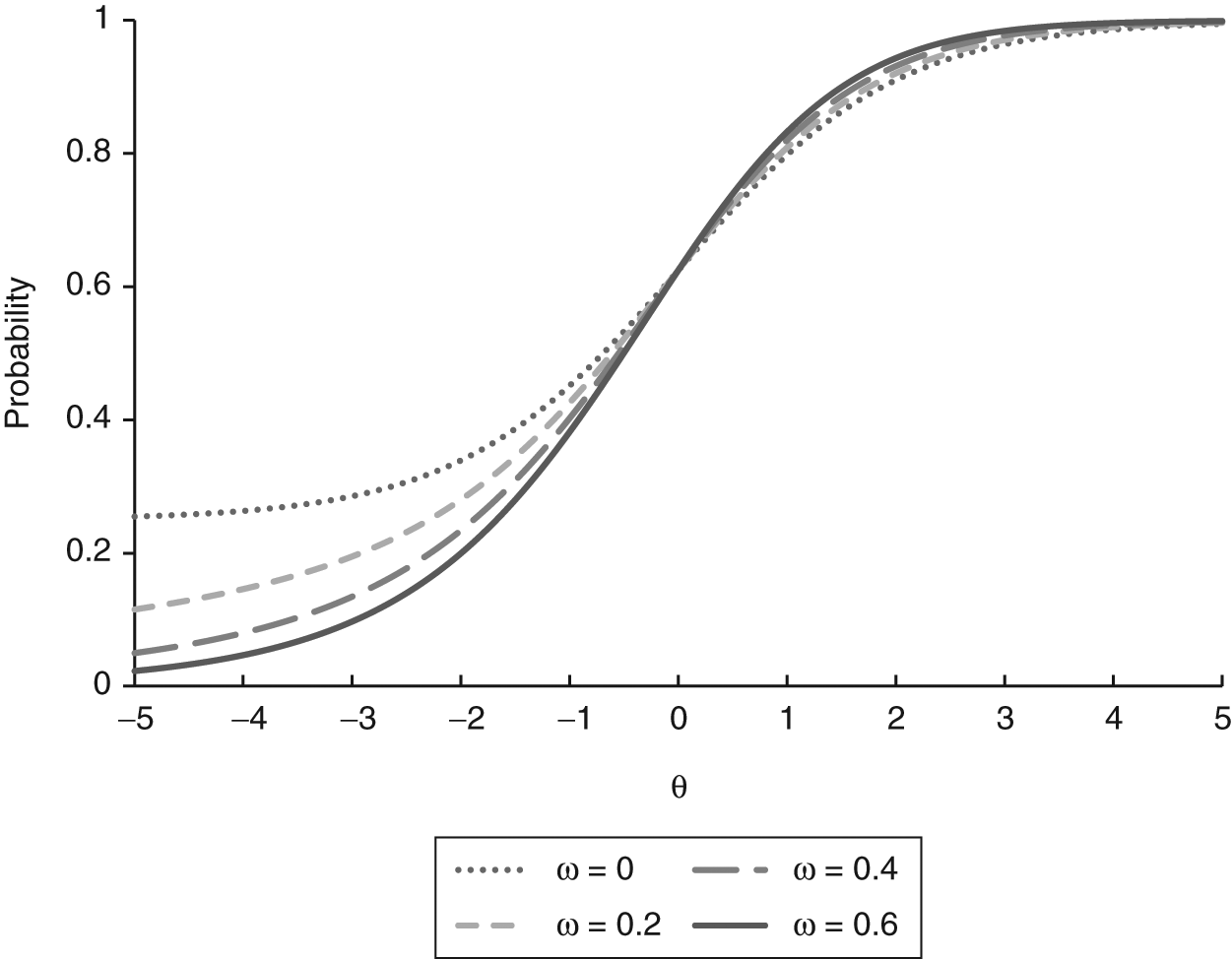
Item characteristic curves for the 1PL-AG (one-parameter logistic model with ability-based guessing) with b = 0, d = −1.098 and different ω values
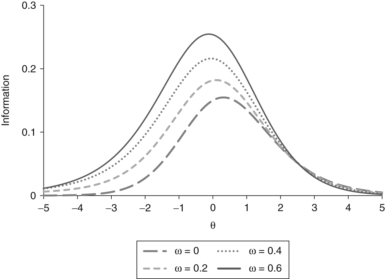
Item information for the 1PL-AG (one-parameter logistic model with ability-based guessing) with b = 0, d = −1.098 and different ω values
The 1PL-AG has ICCs that are very similar to those of the one-, two-, and three-parameter logistic models. This is expected because all models are developed to describe dichotomous item responses. However, the 1PL-AG is formulated in a very different conceptual framework from that of the 3PLM, because it is believed that ability plays a role in guessing. According to San Martin et al. (2006), the parameters of the 1PL-AG can be well recovered in a series of simulations using the SAS NLMIXED computer program (in our experiences, the parameters of the 1PL-AG can also be recovered very well using the freeware WinBUGS; Spiegelhalter, Thomas, & Best, 2003); the 1PL-AG has a better fit to eight empirical data sets of a language test and a mathematics test than the 1PL-G, and the ω values were between 0.036 and 0.246. For more properties of the 1PL-AG and the empirical examples, the reader is referred to San Martin et al. (2006).
Item Selection Procedures
There are many item selection procedures in CAT and CCT. In this study, we developed four major procedures for the 1PL-AG, namely, the Fisher information method (FI), the Fisher information with a posterior distribution method (FIP; Veerkamp & Berger, 1997), the progressive method (PG; Revuelta & Ponsoda, 1998), and the adjusted progressive method (APG; Barrada, Olea, Ponsoda, & Abad, 2008). In FI, an item is selected because it has the largest information about the provisional ability estimate. FI is effective if the provisional ability estimate is close to the true ability. In the early stages of CAT or CCT, the provisional ability estimate is often not very close to the true ability, so that FI may not be very efficient. A solution to this problem is to impose a posterior distribution as a weight function, so that the entire range of ability levels, instead of a point, is considered. This solution is the key idea of FIP.
FI is not capable of controlling the item exposure rate. Hence, a small portion of items in the item bank is often used excessively, whereas the other items are used rarely. PG resolves this problem of uneven item exposure by adding randomness to FI. In the early stages of adaptive testing, randomness plays an important role in item selection. As adaptive testing proceeds, randomness becomes less and less important, whereas the Fisher information criterion becomes more and more important. PG consists of the following steps:
Based on the provisional ability estimate, compute the Fisher information for all items not yet been administered in the item bank, denoted as Ii for item i. Draw a random number Ri from a uniform distribution between 0 and max Ii for each item.
Define the weight of location Wh = h/K, where h is the number of items that have been administered for the time being, and K is the fixed maximum test length. For example, for a test with 10 items, the weight of the first item W1 = 0/10, and the weight of the second item W2 = 1/10, and so on.
Compute the weight of an item not yet been administered in the item bank as
As can be seen in Equation (6), Wh defines the importance of the Fisher information component, relative to the randomness component. An item i with the maximum value of Wi is the candidate for administration.
Repeat Steps 1 to 3 until the maximum test length is achieved.
PG is able to reduce item overexposure and increase item bank usage, because it allows randomness to play a more important role in item selection at an earlier stage of adaptive testing. In PG, the importance of randomness in item selection reduces linearly as adaptive testing proceeds, because Wh is defined as h/K. To be flexible, the importance of randomness can reduce at different rates as adaptive testing proceeds. In APG, an acceleration parameter t is adopted to adjust the weight value Wh:
where t is the acceleration parameter that permits control of the speed with which Wh, moves away from 0 for the first item to reach 1 for the last item; b is a bound variable, used only for calculations; and K and h are defined as above. The larger the acceleration parameter, the smaller the value of Wh, and thus the longer the impact for the randomness component on item selection, as shown in Figure 3 where 10 items are administered. A zero of the acceleration parameter indicates a linear transition between the randomness component and the Fisher information component, that is, the PG method. If one wishes to increase the importance of randomness on item selection in order to increase bank usage and test security, then the acceleration parameter should be set at a larger positive value (e.g., 2). On the other hand, if one wishes to increase the importance of item information in order to increase measurement precision, then the acceleration parameter should be set at a larger negative value (e.g., −2).
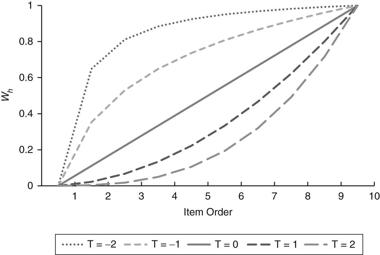
W h with different acceleration parameters for 10 items
Termination Criteria in Computerized Classification Testing
In addition to item selection methods, the termination criterion, which is an algorithm that determines whether an examinee can be classified (i.e., whether the test can be terminated), is another critical component in CCT. There are two major termination criteria in CCT. The sequential probability ratio test (SPRT; Eggen, 1999; Wald, 1947) formulates the decision process as a hypothesis test in which the examinee’s ability estimate is equal to a specified point above the cut score or another specified point below the cut score. On the other hand, the ability confidence interval method (ACI; Thompson, 2009), originally termed adaptive mastery testing (Kingsbury & Weiss, 1983), terminates the test when a confidence interval for the examinee’s ability estimate is completely above or below the cut score.
After reviewing several item selection algorithms in CCT, Thompson (2009) concluded that there is no substantial superiority of a single method, because some of the methods actually assess items very similarly despite different calculations and usually select the same item. Therefore, consideration of methods that assess information across a wider range is often unnecessary under realistic conditions (e.g., when item expose control, content balancing, or operations constraints are imposed), although it might be advantageous to use them in the early stages. In addition, the efficiency of item selection methods depends on the termination criteria that are used. In general, the current ability estimate item selection methods (an item with the maximum information at the current ability estimate should be administered) should be used together with the ACI, whereas the cut score item selection methods (an item with the maximum information at the cut score should be administered) should be used together with the SPRT. We followed this suggestion in this study.
Originally developed in 1947, the SPRT has become a popular classification criterion in CCT. As in hypothesis testing, there are a null hypothesis and an alternative hypothesis in the SPRT, H0: θ = θ0, and H1: θ = θ1, where θ0 and θ1 are the lower bound and upper bound of the cut score, respectively. The following likelihood ratio is then computed:
where
In the ACI, we compute 100(1 − α)% confidence interval of the ability θ:
where θ can be estimated as the expected value of the posterior distribution; SE is the standard error (i.e., the standard deviation of the posterior distribution); zα/2 = 1.96, if α = .05. If the cut score is smaller than the lower bound l, then the examinee is classified as in Category 2 (mastery); if the cut score is larger than the upper bound u, then the examinee is classified as in Category 1 (nonmastery); if the cut score falls between l and u, another item is administered until the maximum test length is reached. If at that time the cut score still falls between l and u, then the examinee will be classified as in Category 1 if
Since the SPRT goes together with the cut score based item selection, only a small subset of items in the item bank will be administered, resulting in a high item exposure rate for some items and a very low bank usage. In contrast, as the ACI goes together with the ability estimate–based item selection, a large subset of items will be administered, so that the item exposure rate will be lower and the bank usage will be higher than those in the SPRT. These differences between the SPRT and ACI are particularly obvious when FI is used and no item exposure control method is implemented.
Both the SPRT and the ACI are popular in CCT. However, their performances cannot be directly compared because they adopt very different settings. In the SPRT, one has to specify a lower bound and an upper bound of the cut score, in addition to the Type I error rate and the Type II error rate. All these settings can affect the performance of the SPRT. In the ACI, one has to specify the Type I error rate only. Kingsbury and Weiss (1983) observed that the SPRT had better efficiency (defined as mean test length) but the ACI had better accuracy (defined as percentage of correct classifications). Spray and Reckase (1996) observed that the SPRT has a better efficiency, given that its accuracy is similar to that of the ACI. Actually, efficiency and accuracy cannot be separated, that is, when comparing one criterion (e.g., efficiency) between the SPRT and the ACI, the other criterion (e.g., accuracy) has to be kept equal between methods. Wang and Liu (in press) compared the performances of the SPRT and ACI under the generalized graded unfolding model (Roberts, Donoghue, & Laughlin, 2000) and observed that the ACI requires a shorter test length than the SPRT to achieve approximately the same accuracy in classification, but at the expense of a higher forced classification rate.
Item Exposure Control Methods
There are many item exposure control procedures. In this study, we adopted the Sympson–Hetter online method with freeze (SHOF; Wu & Chen, 2008), which is an online and freeze extension of the Sympson and Hetter (1985) method. In this method, a random number is first generated from a uniform distribution between 0 and 1, and then it is compared with the item exposure parameter. The item is administered if its exposure parameter is greater than the random number; otherwise, another new item is selected from the item bank. This method requires intensive simulation prior to “real” adaptive testing. Moreover, the item exposure parameters are population dependent, that is, if the distribution of the “real” population does not match that of the population used to derive the item exposure parameters, then the item exposure may not be well controlled. To resolve these problems, Jhu and Chen (2008) developed the Sympson–Hetter online method, which is cost effective and population independent because the item exposure parameters are derived on the fly. However, because the Sympson–Hetter online method cannot control item exposure very well at early stages of CAT, Chen, Lei, and Liao (2008) developed the SHOF.
Let P(S) be the probability of an item being selected; P(A) be the probability of an item being administered; P(A/S), the item exposure parameter, be the probability of an item being administered conditional on being selected; and rmax be the prespecified maximum exposure rate (in this study, 0.2). Our goal is to make P(A), which is equal to P(S) × P(A/S), be no greater than rmax:
Set all item exposure parameters to 1 as an initial value. Then, the SHOF starts as follows:
When an examinee is to respond to the jth item, based on the recently estimated ability (
After administering the jth item, based to the examinee’s item response, update the ability estimate.
Repeat Steps 1 and 2 until the person completes the test (K items).
When an examinee completes the test, compute P(S) and P(A) for each item. Based on the updated P(S), reset P(A/S) for each item in the bank as follows: if P(A) > rmax, then set P(A/S) as 0 to freeze the item (i.e., no longer available for administration); if P(S) > rmax > P(A), then set P(A/S) as rmax/P(S); if
Repeat Steps 1 to 4 until all examinees complete the test.
Two Simulation Studies
We conducted two simulation studies to evaluate the performances of these CCT algorithms under the 1PL-AG. The SPRT and the ACI were implemented in both studies. Study 1 focused on the comparison of FI, FIP, PG, and APG across different weights of ability on guessing (ω). In Study 2, the SHOF was implemented to control item exposure, and the four item selection methods were compared across different weights of ability on guessing. The performances were evaluated with the following criteria: correct classification rate, forced classification rate, bank usage, maximum item exposure rate, and summary statistics (mean and SD) of test length across those examinees who had been classified before the maximum test length of 60 items was reached.
Study 1: Comparison of Four Item Selection Methods Without Item Exposure Control
Design
The item bank consisted of 360 items following the 1PL-AG. The difficulty parameters were generated from N(0, 1) and the d parameters from U(−3.16, −1.098). According to Equation (4), a d-parameter of −3.16 and −1.098 corresponded to a c-parameter of 0 and 0.25, respectively, under the 1PL-AG. A total of 10,000 examinees were generated from N(0, 1). The acceleration parameter of APG was set at 1, indicating a longer impact for the random component on item selection than PG, where the acceleration parameter was zero. The person ability was estimated with expected a posteriori. The value of ω was set at 0, 0.2, 0.4, and 0.6, representing zero to large effects of ability on guessing. The maximum test length was 60 items. There were two categories to be classified with a cut score of zero. In the SPRT, θ0 = −0.25, θ1 = 0.25, α = .05, β = .1; in the ACI, α = .05.
It was expected that the larger the value of ω, the better the classification would be. The four item selection methods (FI, FIP, PG, and APG) would produce similar degrees of accuracy in classification, but FIP, PG, and APG would have a better bank usage and a better item exposure control than FI.
Results
The upper part of Table 1 summarizes the results for the four item selection methods when the SPRT was used for classification. It appears that these four methods yielded almost identical correct classification rates (.91-.92) and forced classification rates (.20-.25), but very different degrees of bank usage. Out of the 30 items in the bank, FI used only 60 items, PG used 137 to 149 items, APG used 102 to 120 items, and FIP used 109 to 131 items; both FI and FIP yielded a maximum item exposure rate of 1, whereas PG and APG yielded a maximum item exposure rate of .77 to .88. The higher bank usage and lower item exposure rate in PG and APG were because randomness played a role in item selection. A closer look at those examinees who were forced to be classified or misclassified, we found that in general the closer the ability to the cut score, the higher the forced classification rate or misclassification rate (detailed results are not shown). For example, when ω = 0.4 and FI was used for item selection, among those who were forced to be classified, 88% of examinees had ability levels within a half standard deviation around the cut score (i.e., −0.5 to 0.5); among those who were misclassified, 96% of examinees had ability levels between −0.5 and 0.5. Similar percentages were found under the other conditions.
Summary Statistics for the Four Item Selection Methods in Study 1
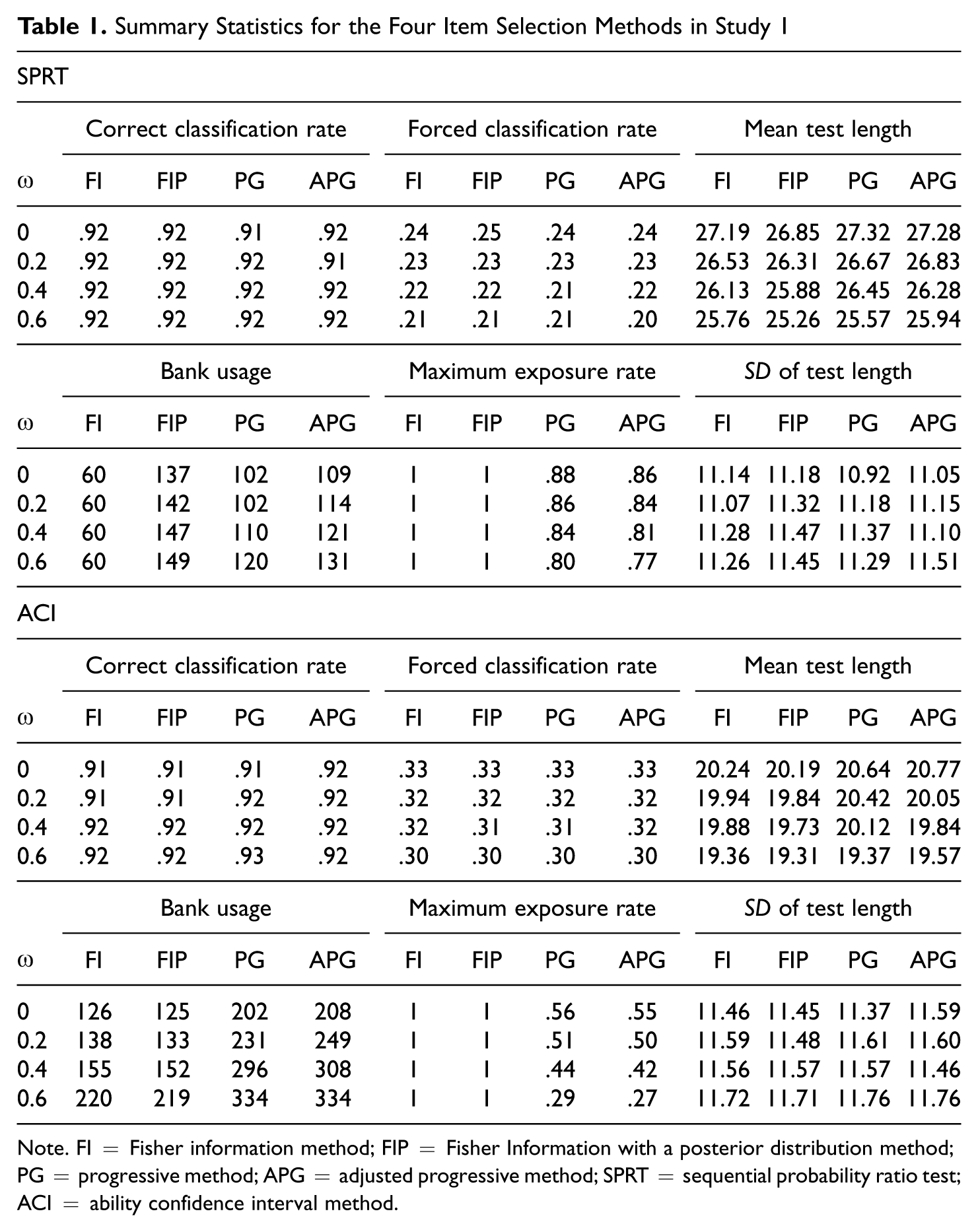
Note. FI = Fisher information method; FIP = Fisher Information with a posterior distribution method; PG = progressive method; APG = adjusted progressive method; SPRT = sequential probability ratio test; ACI = ability confidence interval method.
After removing those who were forced to be classified, we observed that the mean test lengths for the four item selection methods were almost identical: 25.76 to 27.19 items for FI, 25.26 to 26.85 for FIP, 25.57 to 27.32 for PG, and 25.94 to 27.28 for APG; the standard deviation of test lengths for the four methods were almost identical as well—between 10.92 and 11.51. All these findings suggested that FIP, PG, and APG were superior to FI in bank usage and item exposure control (for PG and APG), without sacrificing substantial accuracy (defined as correct classification rate) or efficiency (defined as test length). The difference between PG and APG appeared to be trivial. With regard to ω, in general, a larger ω led to a lower forced classification rate, a shorter test length, a better bank usage, and a smaller item exposure rate.
The lower part of Table 2 summarizes the results for the four item selection methods when the ACI was used for classification. As found in the SPRT, the four methods yielded almost identical correct classification rates (.91-.93) and forced classification rates (.30-.33), but different degrees of bank usage. Of the 30 items in the bank, FI used 126 to 220 items, FIP used 125 to 219 items, PG used 202 to 334 items, APG used 208 to 334 items. The maximum item exposure rate was 1 for both FI and FIP, but only .29 to .56 for PG and .27 to .55 for APG. Like the SPRT, the closer the ability to the cut score, the higher the forced classification rate or misclassification rate. For example, when ω = 0.4 and FI was used for item selection, among those who were forced to be classified, 82% of examinees had ability levels between −0.5 and 0.5; among those who were misclassified, 97% of examinees had ability level between −0.5 and 0.5. Similar percentages were found under the other conditions.
Summary Statistics for the Four Item Selection Methods With the SHOF in Study 2
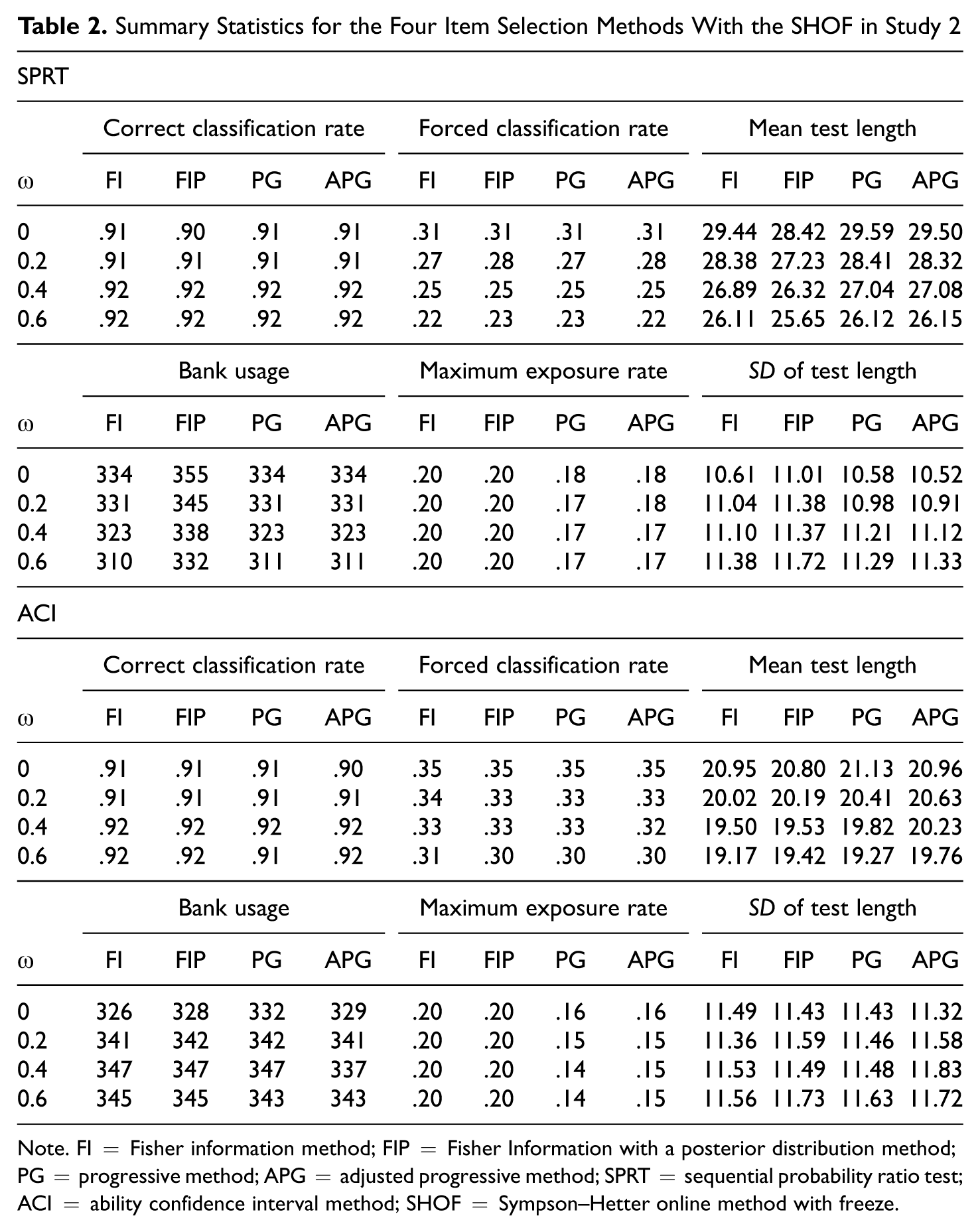
Note. FI = Fisher information method; FIP = Fisher Information with a posterior distribution method; PG = progressive method; APG = adjusted progressive method; SPRT = sequential probability ratio test; ACI = ability confidence interval method; SHOF = Sympson–Hetter online method with freeze.
After removing those examinees that were forced to be classified, we found that the mean test lengths for the remaining examinees were 19.36 to 20.24 items for FI, 19.31 to 20.19 for FIP, 19.37 to 20.64 for PG, and 19.57 to 20.77 for APG. The standard deviations of test lengths were 11.37 to 11.76 for the four methods. Thus, all the four item selection methods performed very similarly in accuracy and efficiency. However, PG and APG appeared to have better bank usage and item exposure control than FI and FIP. As found in the SPRT, in general a larger ω resulted in a lower forced classification rate, a shorter test length, a better bank usage, and a smaller item exposure rate (for PG and APG only). Moreover, it appeared that a larger ω generated a slightly higher correct classification rate as well, which was not as obvious in the SPRT.
The performance of the SPRT depends on the Type I error rate α, the Type II error rate β, cut score, and indifference region; whereas the performance of the ACI depends on the Type I error rate and cut score. Thus, their performances may not be directly comparable. To make a comparison between these two methods, a pilot simulation study was conducted to explore these parameters α, β, cut score, and indifference region so that the correct classification rates of the SPRT and ACI would be similar. Given that the SPRT and ACI performed very similarly in correct classification rate (i.e., accuracy), the test lengths can be used to compare the efficiency of the two methods. Compared with the SPRT, the ACI had a shorter test length, a larger bank usage, a lower item exposure rate, but a larger forced classification rate. Thus, the ACI seemed to be slightly more efficient than the SPRT, but at the expense of a larger forced classification, which is consistent with the literature (Wang & Liu, in press).
The correct classification rates were approximately .91 to .93 for the SPRT, indicating there were approximately 7% to 9% error rates, which were much lower than the sum of the Type I and Type II error rates in the SPRT. This was consistent with the literature (Eggen, 1999; Eggen, & Straetmans, 2000), suggesting there are other factors than the nominal error rates that affect the performance of the SPRT (e.g., cut score).
Study 2: Comparison of Four Item Selection Methods With the SHOF for Item Exposure Control
Design
The simulation design was identical to that of Study 1, except that the SHOF was implemented with a maximum item exposure rate of .2 here. It was expected that the item exposure would be better controlled; all item selection methods would perform more similarly; the bank usage would be increased; the correct classification rate would not decrease substantially but the test length would perhaps increase slightly, as compared with those in Study 1, where no item exposure control was implemented.
Results
The upper part of Table 2 summarizes the results for the four item selection methods when the SPRT was used for classification. As expected, the maximum item exposure rates for the four methods were controlled at the prespecified value of .2. The four methods performed almost identically. They yielded very similar correct classification rates (.91-.92), forced classification rates (.22-.31), and bank usage (310-355 items). After removing those examinees that were forced to be classified, we found that the test lengths for the remaining examinees were very similar across the four methods, with means between 25.65 and 29.59 items, and standard deviations between 10.52 and 11.72.
The lower part of Table 2 summarizes the results for the four item selection methods when ACI was used for classification. The maximum item exposure rates were well controlled at the prespecified value of .2. The four methods performed very similarly in correct classification rates (.90-.92), forced classification rates (.30-.35), bank usage (326-347 items), and mean (19.17-21.13 items) and standard deviation (11.32-11.83) of test lengths. Given that the SPRT and the ACI performed very similarly in accuracy, we were able to compare their relative efficiency. Compared with the SPRT, the ACI required a shorter test length but generated a larger forced classification rate.
As found in Study 1, in general, a larger ω resulted in a lower forced classification rate, a shorter test length, and a slightly higher correct classification rate; the closer the ability to the cut score, the higher the chance of forced classification or misclassification. A comparison of Tables 1 and 2 reveals that the implement of the SHOF generated little loss in accuracy and efficiency in that the correct classification rates and the test lengths remained almost unchanged.
Conclusions and Discussion
Most CAT and CCT algorithms were developed for MC items, because MC items rather than constructed response items can be scored by computers in real time. In addition, most CAT and CCT algorithms assume the 3PLM, because the 3PLM is widely fit to MC items. The major justification of the 3PLM for MC items is the incorporation of the pseudoguessing parameter, which is an item characteristic and independent of a person’s ability. In reality, guessing often involves ability: The more capable an examinee, the wiser the guessing. In other words, guessing depends on ability. The 1PL-AG was developed to address this concern.
As an IRT model, the 1PL-AG is eligible for CAT and CCT, which has not yet been implemented in the literature. In this study, we have successfully developed CCT algorithms under the 1PL-AG, including the cut score–based SPRT and the ability estimate–based ACI termination procedures; the FI, FIP, PG, and APG item selection methods; and the SHOF item exposure control procedure. Two simulation studies were conducted to assess the performances of these algorithms. Several conclusions are drawn. First, both the SPRT and ACI are feasible with correct classification rates above .90, but the ACI requires a shorter test length than the SPRT to achieve the same level of accuracy, at the expense of a higher forced classification rate. Second, FI, FIP, PG, and APG perform very similarly in accuracy and efficiency of classification, but FIP, PG, and APG outperform FI in terms of better bank usage and item exposure control. Third, the SHOF can maintain item exposure at a prespecified rate, without compromising substantial accuracy and efficiency. Fourth, once the SHOF is implemented, FI, FIP, PG, and APG perform almost identically in every aspect. Fifth, in general, a higher weight of ability in guessing generates both higher accuracy and efficiency and a lower forced classification rate. Finally, the closer the ability to the cut score, the higher the probability of forced classification or misclassification.
Several issues need to be investigated further before CAT and CCT under the 1PL-AG are put into operation. There are only two categories (e.g., mastery and nonmastery) in this study. In some cases, more categories may be required (e.g., A, B, C, and D grades). It would be of great value to develop the SPRT and ACI and evaluate their performances when there are more than two categories. CAT under the 1PL-AG has not yet been developed. Issues in simultaneous control of item exposure and test overlap (Chen et al., 2008; Chen & Lei, 2005), content balancing, and other practical constraints (Cheng, Chang, & Yi, 2007; van der Linden & Veldkamp, 2004) need to be revisited under the 1PL-AG. Recent modifications in the SPRT are also noteworthy (Bartroff, Finkelman, & Lai, 2008; Thompson, 2010).
Footnotes
The authors declared no potential conflicts of interests with respect to the authorship and/or publication of this article.
This work was supported by a start-up research grant No. RGB32/2008-2009 from The Hong Kong Institute of Education.