
Abstract
Standard setting is a method used to set cut scores on large-scale assessments. One of the most popular standard setting methods is the Bookmark method. In the Bookmark method, panelists are asked to envision a response probability (RP) criterion and move through a booklet of ordered items based on a RP criterion. This study investigates whether or not it is possible to end up with the same cut scores if one were to apply the Bookmark method with two different RP values. Analytical formulas and two hypothetical examples from a large-scale state testing program indicate that it is rarely possible to obtain the same cut score estimates with two different RP values because of the presence of item difficulty gaps present when applying the procedure in practice. Results indicate that if the same group of panelists applied the Bookmark procedure as it is traditionally explained, then cut scores should be lower with the second chosen RP value than they were with the first RP value. This result holds whether or not the second RP value is higher or lower than the first RP value. The examples also reveal that differences in cut score estimates with different RP values can lead to changes in the percentage of examinees at or above the cut scores that may have important practical impacts.
Keywords
Introduction
Recent years have seen the increased use of large-scale assessments for high-stakes decision making. Specifically, assessments are increasingly being used for making licensure, certification, school accountability, and retention/promotion decisions. Most of these high-stakes decisions are based on cut scores established through the application of a standard setting procedure. Among the available methods for setting cut scores, the Bookmark standard setting procedure (Lewis, Mitzel, & Green, 1996; Lewis, Mitzel, Green, & Patz, 1999; Mitzel, Lewis, Patz, & Green, 2001) has become increasingly popular, primarily because of the ease of application and the perceived simplicity of the standard setting task (Karantonis & Sireci, 2006) in comparison with other commonly used standard setting methods, such as the Angoff procedure (Angoff, 1971).
In the Bookmark method, panelists move through a booklet of test items ordered from the easiest to the hardest according to a specific probability level to indicate a cut score (Lewis et al., 1996; Lewis et al., 1999; Mitzel et al., 2001). The booklet of ordered test items is called an ordered item booklet (OIB) and it serves as the stimuli that panelists use when providing their judgments. The specific probability level used to order the items in the OIB is known as the response probability (RP) criterion. It is the probability level at which a minimally competent examinee (MCE), an examinee who just possesses the necessary knowledge, skills, and abilities to meet the standard, should obtain that score or higher. For example, if the RP value is 0.67 and the items are multiple-choice items that are scored correct or incorrect, then the MCE should have at least a 67% chance of getting the items correct if the items are before the bookmark and a less than 67% chance of getting the items correct if the items are after the bookmark.
The first step in Bookmark standard setting is to consider the performance level descriptors (PLDs) for each cut score that needs to be set on the assessment. The PLDs describe that which MCEs should be able to do if they were classified into that performance category (Perie, 2008). After discussing the PLDs and what they mean, the Bookmark standard setting process is typically explained. This process consists of explaining the concept of the RP criterion and how it is used to move through the OIB and indicate a cut score. Specifically, panelists are usually instructed that the items are in order from the easiest to the hardest and that their task is to consider each test item, the PLDs, and the MCEs that they are familiar with and ask themselves whether or not they think that the MCEs have a probability of obtaining that score or higher that is greater than or equal to the RP criterion. If the answer is no, they bookmark the item. If the answer is yes, they move to the next item and ask the same question.
Since in operational settings locating the item to bookmark is a difficult task, panelists are often encouraged to move a couple of items past their initial bookmark to make sure that the bookmark represents their best judgment of the cut score (ACT Inc., 2005). The ultimate task of the panelists is to select the item in the OIB that they think separates what the MCE should know and be able to do from what they should not know and be able to do. The θ value of the bookmarked item is the panelist’s cut score estimate. The group cut score estimate is either the mean or the median of the individual panelists’ cut score estimates. This process is typically repeated over several rounds with various forms of feedback provided after each round (Reckase, 2001).
Even though the Bookmark procedure is perceived to be simpler than some other standard setting methods (Karantonis & Sireci, 2006; Lewis et al., 1996; Lewis et al., 1999; Mitzel et al., 2001), it is still a very difficult process for panelists, and there are complications and challenges associated with its application. One such challenge is that there is not one unique criterion that underlies test performance (Haertel & Lorié, 2004). In particular, it is possible to design the OIB based on any RP level between 0 and 1. In practice, an RP value greater than or equal to 0.50 is typically chosen since values greater than or equal to 0.50 are assumed to represent mastery (Haertel & Lorié, 2004). The decision to use a particular RP value is often made by the policy makers responsible for setting standards and defining standard setting policy. The two most common RP values are 0.50 (RP50) and 0.67 (RP67; Huynh, 2006), but values between 0.50 and 0.80 have been used (Huynh, 2006; Karantonis & Sireci, 2006; Um, Way, Fitzpatrick, & Kreiman, 2009; Zwick, Senturk, Wang, & Loomis, 2001).
There are two critical observations associated with the choice of a RP value. First, there is the possibility that the order of the items in the OIB will change with different RP values (Beretvas, 2004; Kolstad, 2002; Kolstad et al., 2001; Skaggs, 2007; Skaggs & Tessema, 2001; Um et al., 2009) when the Rasch model is not used to scale the test. For example, if an item is the sixth most difficult item under one RP value, it may not be the sixth most difficult item under a different RP value. Second, the use of a RP value creates gaps along the score scale where it is not possible for an individual panelist to set a cut score. These gaps are referred to as item difficulty gaps or score gaps (Cizek & Bunch, 2007; Reckase, 2006). An important realization has been that these gaps can impact estimated cut scores. Cizek and Bunch (2007) point out that when there are large item difficulty gaps, it can make it difficult to accurately estimate cut scores. They call for more research into the impact of item difficulty gaps.
An important and yet unanswered question in this context is how the item difficulty gaps interact with changing the RP values to impact estimated cut scores. Is it possible to obtain the same cut score when different RP values are chosen? Hambleton and Pitoniak (2006) state that:
In theory, panelists using a lower RP value such as 0.50 would place the bookmark later in the ordered item booklet than panelists using a higher RP value such as 0.80. However, the performance standard connected with the bookmarked items would theoretically be equivalent, leading to identical standards. (p. 443)
They further observed that empirical research with different RP values resulted in disparate cut scores. They cite a study by the National Research Council (2005) using RP values of 0.50, 0.67, and 0.80 and another study by Williams and Schulz (2005) using RP values of 0.50 and 0.67 as examples of studies where empirically derived cut scores turned out to be discrepant with different RP values. These researchers observed that higher RP values tended to lead to higher estimated cut scores. This suggests that the question or whether or not it is possible to obtain the same cut scores with different RP values still remains.
The purpose of this article is to clarify Hambleton and Pitoniak’s (2006) statement and provide the exact conditions under which identical cut scores can be obtained with the Bookmark procedure when using different RP values. This includes showing that certain parameters are required of items in the OIBs to obtain identical cut scores. Since OIBs used in practice rarely satisfy these conditions, the question of how close the cut scores can be with different RP values is also investigated. Two empirical examples based on data from a large-scale state testing program, one using the Rasch model and the other using the three-parameter logistic (3PL) model, guide these investigations. These examples demonstrate an important finding that if the same group of panelists was instructed to use the Bookmark procedure as it has traditionally been explained with two different RP values, one should expect that cut score with the second RP value to be lower than the cut score with the first RP value. This result is a function of the definition of a RP value and is contrary to what has been observed in the National Research Council (2005) and Williams and Schulz (2005) studies. Results also suggest that differences between the cut scores and the percentage of students who would be at or above the cut scores (percentage at or above cut [PAC]) with alternate RP values in some cases may be larger than one might expect and may have important practical impacts. The article concludes with discussion and some additional considerations when applying the Bookmark method in the future.
Determining Bookmark Locations
To theoretically investigate whether or not cut scores can be identical with different RP values, one can examine the analytical Bookmark location formulas presented by Beretvas (2004). Beretvas outlined a series of formulas that could be used to determine the θ locations for the Rasch model, the 2PL model, the 3PL model, the generalized partial credit model (GPCM) with up to five score categories, and the graded response model (GRM). These formulas are found by solving for θ in the formulas for each of the item response theory (IRT) models, respectively, assuming a particular RP value. A unique feature of these formulas is that they are a function of both the RP value and the item parameters of the item.
Specifically, Beretvas (2004) showed that the Bookmark location of an item in the OIB under the Rasch model is

where RP is the RP criterion chosen (e.g., 0.50, 0.67, 0.80) and b is the Rasch difficulty parameter. For the 3PL model, the formula for the Bookmark location of the item is

where RP again is the RP criterion chosen (e.g., 0.50, 0.67, 0.80), a is the discrimination parameter, b is the difficulty parameter, c is the pseudo-guessing parameter, and D is a scaling constant that is approximately equal to 1.7. The analytical formulas for the 2PL, GRM, and GPCM are discussed in Beretvas (2004). For simplicity, only the formulas for Rasch and 3PL models are presented in this article.
Implications of Bookmark Location Formulas
One expects then, if the statement by Hambleton and Pitoniak (2006) universally holds, that cut scores with different RP values should be identical no matter the RP value chosen because a panelist should be able to move his or her bookmark back in the OIB with the lower RP value and bookmark an item that would result in the same cut score. However, Equations (1) and (2) suggest that it is not always the case. For example, consider a Rasch item with a b parameter of 1.000. This item would be located at a scale location of 1.000 with RP50. The same item would be located at a scale location of approximately 1.708 with RP67. This implies that if one were to bookmark this item under the two different RP values, it would result in two different cut scores. It also implies that if a person bookmarked this item with RP67 to end up with the same cut score with RP50, the RP50 OIB must contain an item with a difficulty parameter of approximately 1.708. Bookmarking the item with a difficulty parameter of 1.708 in the RP50 OIB would translate into the same cut score as bookmarking the item with a difficulty parameter of 1.000 in the RP67 OIB. This shows that to end up with the same cut score under different RP values, the OIB must contain items with specific sets of item parameters or else the cut scores will differ. The appendix shows the formulas of items needed with the Rasch and 3PL models to end up with the same cut scores with two different RP values.
A key realization is that in practice OIBs do not typically contain items that will be located at the same scale locations with different RP values. This means that in practice, where the OIBs typically contain less than 100 items, differences in θ values and cut scores should be expected if different RP values are applied. These differences occur because of the presence of the item difficulty gaps along the score scale when using a RP value to locate items in the OIB and the fact that there may not be items at the same locations with different RP values.
The examples that follow investigate the important question of how similar the cut scores could be with different RP values. Given the findings in National Research Council (2005) and Williams and Schulz (2005) studies, one predicts that the cut scores would be higher with a higher RP value. One might also predict that different RP values would result in fairly similar cut scores since one RP value is not universally preferred in research or practice.
Standard Setting Data
To examine how close cut scores could be with different RP values and whether the cut scores should be expected to be higher with a higher RP value; two examples of possible cut scores with RP50 and RP67 from a large-scale assessment program are provided. These examples were chosen because they are representative of the Bookmark standard setting processes used in the state from which they were drawn in terms of the number of items, IRT models applied, and number of cut scores that need to be set. Other testing programs may use slightly different Bookmark standard setting processes than this state, but as a whole, the examples are fairly typical of many applications.
The first example is drawn from a fifth grade science assessment. The Grade 5 science assessment contains 35 multiple-choice items, which are scaled with the Rasch model. When cut scores were set, the Bookmark standard setting procedure was used with RP50. A group of 14 teachers, parents, and administrators from the state participated in the Bookmark standard setting. These panelists recommended two cut scores with the first cut score used for school accountability purposes.
The standard setting process included three rounds with discussion and feedback between each round. Between the first and second round, panelists were given information on the p values of the items, their own cut score rating, and the cut score estimate for the group of panelists. Between the second and third round of judgments, panelists received additional information on the PAC. In the example that follows, information on the panelists’ bookmarked page from the third rounding of standard setting as well as representative item parameters from the science assessment are used to show the similarity of potential cut score estimates with RP50 and RP67. Information on the PAC is also used to quantify the practical impact of the differences in RP50 and RP67 cut scores for the group of panelists.
The second example is drawn from a Grade 11 reading assessment. The reading assessment has 70 multiple-choice items, which are scaled using the 3PL model. Similar to the Grade 5 science assessment, panelists who participated in the Bookmark procedure applied RP50. The standard setting panel included 15 teachers, parents, and administrators from the state. The panelists recommended three cut scores to separate students into four performance categories. The second cut score is used for school accountability purposes.
The standard setting process for the reading assessments was very similar to the process used for the science assessments in terms of the number of rounds and the types of feedback used in the standard setting. Similar to the science assessment, information on the page panelists bookmarked in the third rounding as well as representative item parameters from the reading assessment were used to determine the potential similarity of cut scores with RP50 and RP67. Information on the PAC is also used to quantify the practical impact of the differences in RP50 and RP67 cut scores for the group of panelists.
Item Locations and Difficulty Gaps
Science Assessment
The scale locations for the 35 multiple-choice items from the Grade 5 science assessment are shown graphically in the item map (i.e., a picture that shows the items and their relationship to the θ locations) in Figure 1 for RP50 and RP67. Since the IRT model applied in this standard setting was the Rasch model, the scale locations are uniformly shifted upward with RP67 in comparison with RP50, and the order of the items in the OIBs do not change. The gaps between consecutive items in the OIBs also stay the same, although the locations of the gaps are again shifted upward with RP67. These are well-known properties of the Bookmark procedure when applying the Rasch model. The upward shifting for RP67 shows that to end up with a similar cut score, a panelist must place his or her bookmark earlier in the OIB with RP67 than he or she does with RP50. Additionally, it is apparent that there are many values on score scale under RP50 that are not present with RP67 and vice versa.
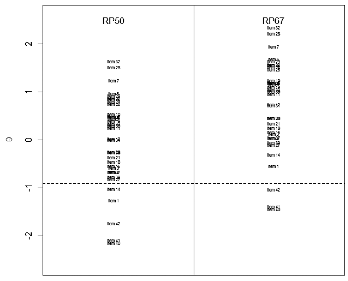
Item map of RP50 and RP67 bookmark locations for science
The dotted line in Figure 1 shows a cut score location of θ = −0.9. Since there is no item handle for RP50 or RP67 that lies directly on the dotted line, it is not possible for a panelist to set his or her cut score at θ = −0.9 with these two RP values. This cut score location lies in an item difficulty gap for both RP50 and RP67.
The specific scale locations of the items and the gaps from Figure 1 are provided in Table 1. The gaps are found by taking the difference between the scale locations of consecutive items in the OIB. For example, the item difficulty gap between the first two items in the OIB is 0.053 since the difference between the scale locations of these two items is 0.053. The gaps reported are uniformly positive and range from approximately 0.000 to 0.485 with a mean of 0.111 and a standard deviation of 0.115.
Bookmark Locations Rasch Science Standard Setting for RP50 and RP67
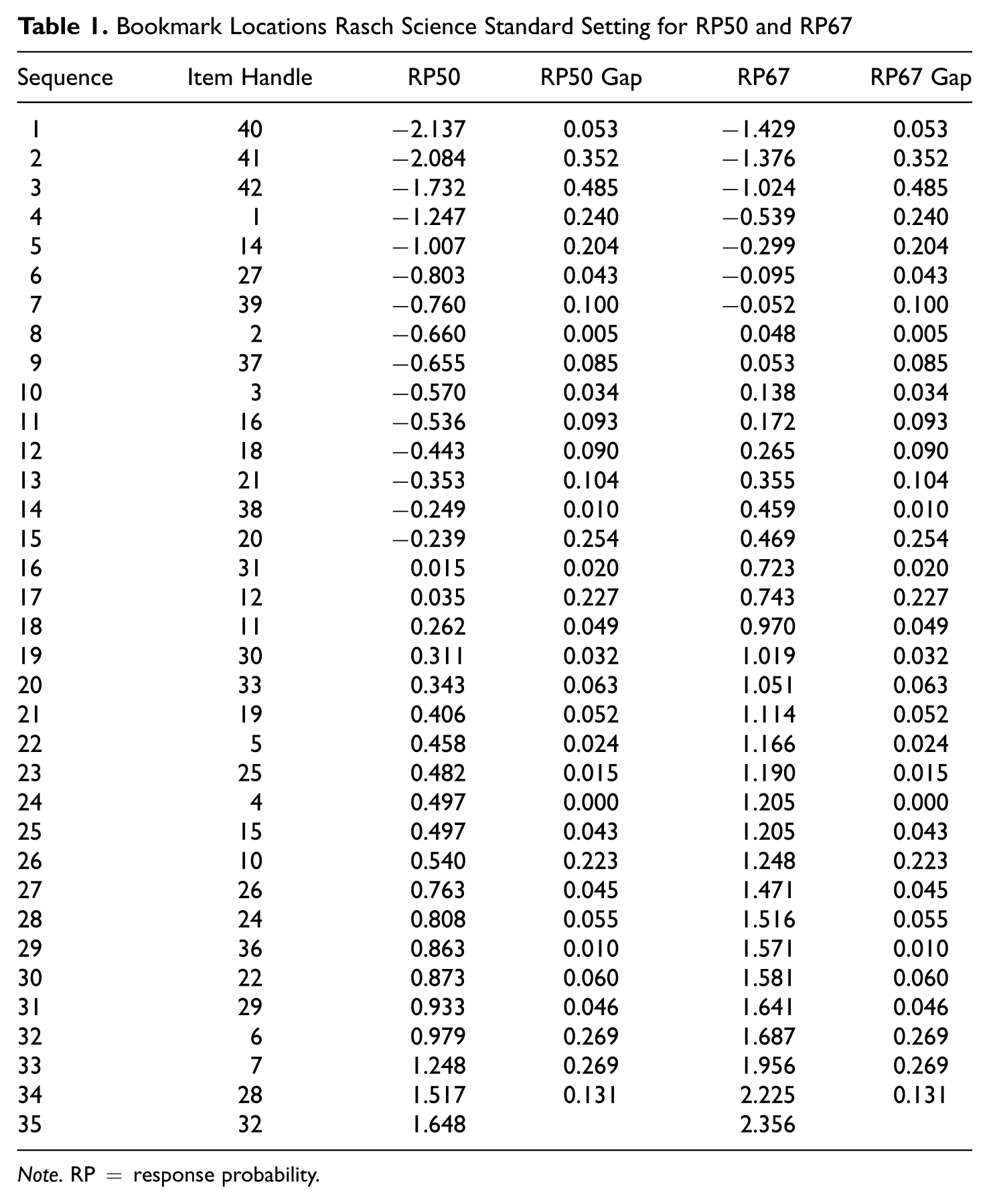
Note. RP = response probability.
Eleventh Grade Reading Assessment
The scale locations for the 70 multiple-choice items from the Grade 11 reading assessment are displayed in the item map in Figure 2. Since the 3PL model is applied as opposed to the Rasch model, the items are shifted upward with RP67 in comparison with RP50 but not necessarily by the same amount. The amount of the upward shift depends on the a and c parameters of items as can be seen in Equation 2. Since the upward shifting of the items depends on a and c parameters, the gaps between consecutive items in the OIBs change under different RP values. Similar to the scale locations in Figure 1, the upward shifting for RP67 shows that to end up with a similar cut score, a panelist must place his or her bookmark earlier in the OIB with the higher RP value. An important observation from Figure 2 that contrasts that in Figure 1 is that the order of the items in the OIBs changes with different RP values. This is a well-known property of OIBs when the IRT model includes a discrimination parameter. Again, similar to Figure 1 many values on the score scale are not present with both RP50 and RP67.
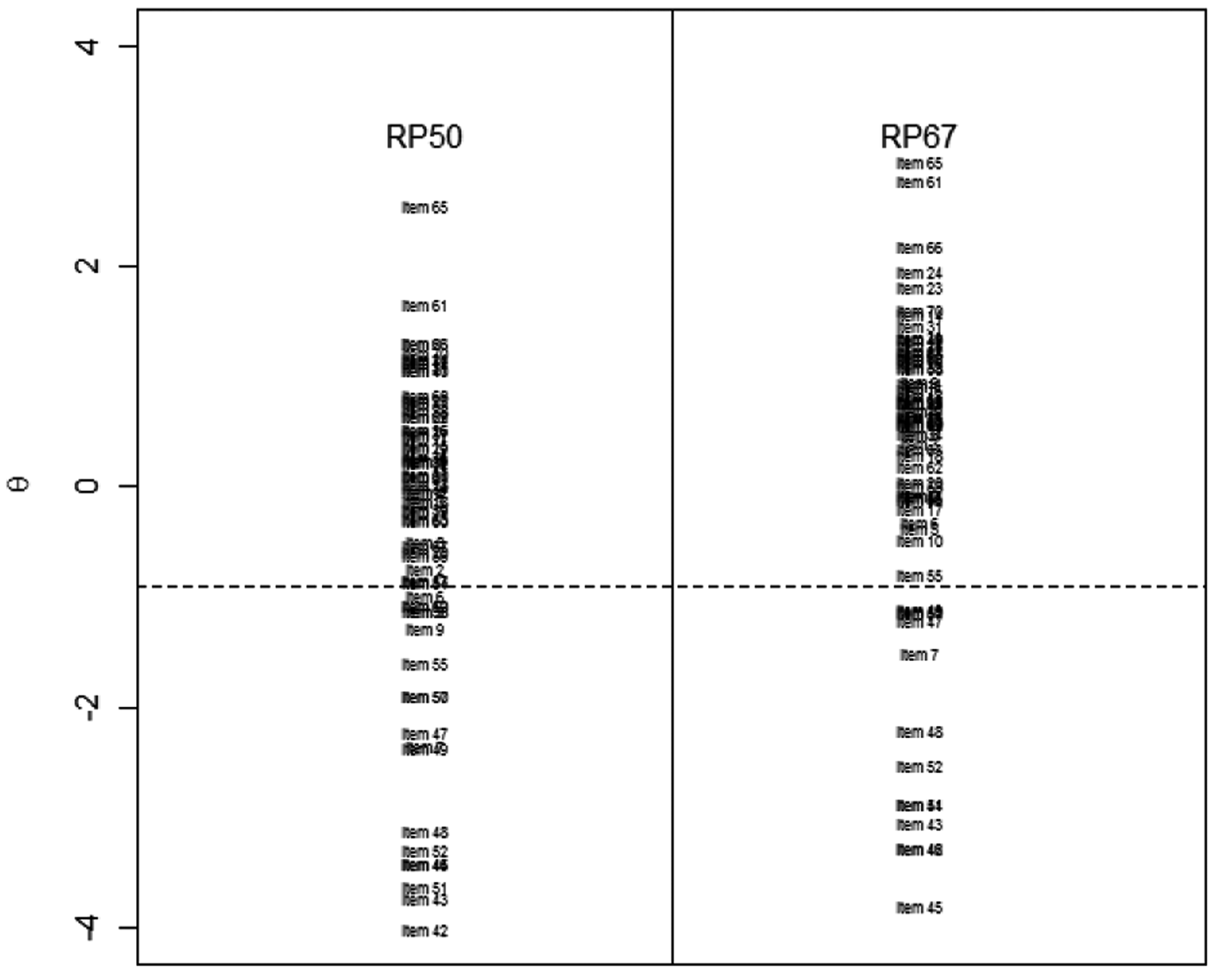
Item map of RP50 and RP67 bookmark locations for reading
The dotted line in Figure 2 again shows a cut score location of θ = −0.9. Since there is no item handle for RP50 and RP67 that lies directly on the dotted line, it is not possible for a panelist to set his or her cut score at θ = −0.9 with these two RP values for the reading assessment. The closeness of the items to the dotted line in the graph is a function of the size of the text used to display the item locations and the actual scale location of the items.
The specific scale locations of the items and the gaps from Figure 2 are provided in Table 2. The gaps again are uniformly positive. The RP50 gaps ranged from approximately 0.000 to 0.904. The RP67 gaps ranged from approximately 0.000 to 0.703. The means and standard deviations were 0.095 and 0.153 and 0.098 and 0.142 for RP50 and RP67, respectively.
Bookmark Locations 3PL Reading Standard Setting for RP50 and RP67

Note. RP = response probability.
The gaps in Tables 1 and 2 are positive as opposed to negative because when a panelist understands the Bookmark task, the location of his or her cut score can be anywhere between the item he or she bookmarked and the next higher item in the OIB. The positive difficulty gap signifies that when the panelist understands the Bookmark task, the actual cut score that the panelist could be conceptualizing could be higher than the cut score that is estimated for them. These positive difficulty gaps are consistent with the simulation results of Reckase (2006), which indicated that there is the potential for the Bookmark procedure to exhibit negative bias.
Method for Determining Cut Scores
To illustrate how the cut scores may be expected to change under different RP values, it was assumed that the cut scores for RP50 were the cut scores recommended in the third round of standard setting for both science and reading. The cut scores for RP67 were then found by assuming that the same panelists performed the Bookmark procedure in the usual way and that they were trying to set their cut scores at their RP50 cut scores but were instead instructed to use RP67 with the same items. For example, if the panelists’ estimated cut score for RP50 was θ = −0.9, it was assumed that this would be the cut score they were trying to set with RP67, and the items were cycled through to determine if the probability of obtaining correct response was equal to or greater than .67 based on this cut score. The first item on which it was found that probability of getting a correct response was less than .67 was taken as the panelist’s bookmark and cut score.
For the cut score estimates for the group of panelists, both the mean and median were used. The mean and median were investigated for the group of panelists because in practice both approaches have been applied to determine cut scores. It is well known that the mean and median can yield different results when the distribution of examinees is not symmetric and there are outliers in the data set. It is expected that there will be differences between cut scores estimated based on the mean and median since these data are not symmetric.
It should be realized that the examples presented here are purely hypothetical, and that in practice, it is highly unlikely that the same group of panelists would be asked to provide cut score recommendations for two different RP values on the same assessment. This does not take away from points of the illustrations, which are to empirically demonstrate what one should expect to happen if a different RP value was chosen, show the similarity of the possible cut scores, and to provide greater clarity into the theoretical properties of the Bookmark method. These points are fundamental given that the Bookmark method is among the most popular standard setting methods used in practice.
Results
Science Assessment
The results for the panelist cut score recommendations for the RP50 and the hypothetical RP67 cut scores for the first and second cut score placements for the science assessment are presented in Tables 3 and 4, respectively. The tables display the estimated cut scores with RP50 and the item difficulty gap associated with the RP50 cut score as well as the hypothetical RP67 cut scores and item difficulty gaps. The mean, median, and standard deviation of the item difficulty gaps, the estimated cut scores with RP50, and hypothetical cut scores with RP67 are also provided in both Tables 3 and 4.
Round 3 Bookmark Science Standard Setting Judgments for First Cut Score
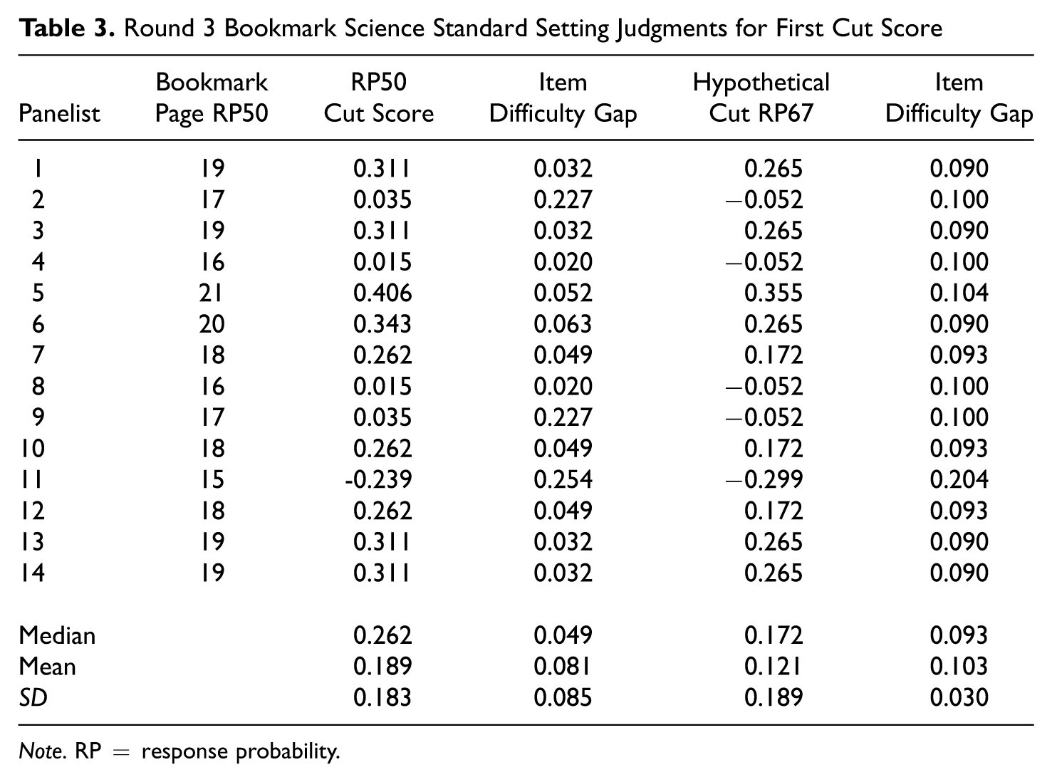
Note. RP = response probability.
Round 3 Bookmark Science Standard Setting Judgments for Second Cut Score

Note. RP = response probability.
A closer examination of Tables 3 and 4 shows that the estimated cut scores under RP67 were uniformly lower than the cut scores estimated with RP50; a finding that is opposite of what one might expect. This occurs because the first item in which the probability will be less than .67 is the first item whose scale location is less than the RP50 cut scores. It is easy to see why this is the case because if the cut score for RP67 was greater than RP50 it would mean that panelists should have placed their bookmark earlier in the OIB for RP50. This means that by definition the scale location of the item for RP67 must be less than RP50. Notice if the panelists started with RP67 and tried to match the RP50 cut score to this cut score then the opposite would be true, the RP67 cut score would be greater than RP50. This result is purely a function of the definition of the RP value and the process that the panelists should use if they were performing the Bookmark method in the traditional manner.
The mean, median, and standard deviation of item difficulty gaps and the panelist cut score estimates provide an indication of the potential impact that the item difficulty gaps and the differences in scale locations have on the cut scores estimated for the group of panelists. For the first cut score with RP50, the group cut score estimate using the mean was 0.189 with a standard deviation of 0.183. For the second cut core, the group cut score estimate was 0.821 with a standard deviation of 0.160. The median group cut score estimates were 0.262 and 0.763 for the first and second cut scores with RP50, respectively. In the context of the cut score estimates, the value of the standard deviations suggests that there is some variation in the cut scores estimated using RP50. The differences between the mean and median show the impact of using different measures of central tendency when the group of panelists’ cut scores is not symmetrically distributed. These differences are common in practical settings. The decision to use the mean or median to determine the group cut score often is a policy decision. The median is often used if one is concerned about the effect of potential extreme panelists, and the mean is often used if one wants all the judgments to contribute to the cut score estimate equally.
The group cut score estimates again were uniformly lower with a higher RP value. This finding again is the opposite of the general findings in the National Research Council’s (2005) report and the study conducted by Williams and Schulz (2005) who observed that the cut scores were higher with higher RP values. The fact that cut scores for the group were lower with RP67 in this example again is a function of the way the cut score is computed. The cut score for a panelist was determined from the first item in which probability of obtaining a correct response is less than .67. The scale of location of this item is less than RP50. Since the panelists’ cut scores were uniformly lower, this means that the group cut scores also were lower with RP67. It is important to point out again that the opposite would be the case if the RP67 was the assumed cut score and one was trying to match the RP50 cut score to this assumed value.
One can quantify the practical impact that using RP50 or RP67 would have on the group cut scores by using information on the PAC observed on the assessment. With the Rasch model, there are a limited number of θ values that are observed (one for each number correct score). This means that one needs to round the hypothetical RP67 cut scores in Tables 2 and 3 to the closest observed θ value. The potential changes in the PAC can then be found by taking the difference in PAC for RP50 and RP67 for each cut score. For the first cut score, the median cut score was 0.262 with RP50 and the median cut score was 0.172 with RP67. This translates into 6.63% more students being at or above the cut score with RP67 on the science assessment. In comparison, the difference in the mean cut scores of 0.189 and 0.121 with RP50 and RP67 translates into 7.98% more students being at or above the cut score with RP67. For the second cut score placement, the differences between the mean and median cut scores translate into 5.88% and 0.00% more students being at or above the cut score with RP67, respectively. The finding that there was no change in the PAC when using the median for the second cut score was a function of the small change in the cut scores (0.763 compared with 0.743) and the fact that these scores end up being rounded to the same θ value when looking up the PAC. The possible 5.88 to 7.98% differences in PAC with RP50 and RP67 for some of the group cut scores are larger than one might expect and suggest that the choice to use RP50 or RP67 could have a big impact on the PAC for these data. Whether or not using RP50 or RP67 will lead to a large or small difference in the PAC in any situation is a function of the cut scores that panelists recommend, the range of θ values that are observed on the assessment, and the distribution of students across those θ values.
Reading Assessments
The results for the panelist cut score recommendations for the RP50 and the hypothetical RP67 cut scores for the three cuts for the reading assessment are presented in Tables 5, 6, and 7. The format and information in the tables is very similar to the information displayed in Tables 3 and 4 for the science assessments.
Round 3 Bookmark Reading Standard Setting Judgments for First Cut Score

Note. RP = response probability.
Round 3 Bookmark Reading Standard Setting Judgments for Second Cut Score
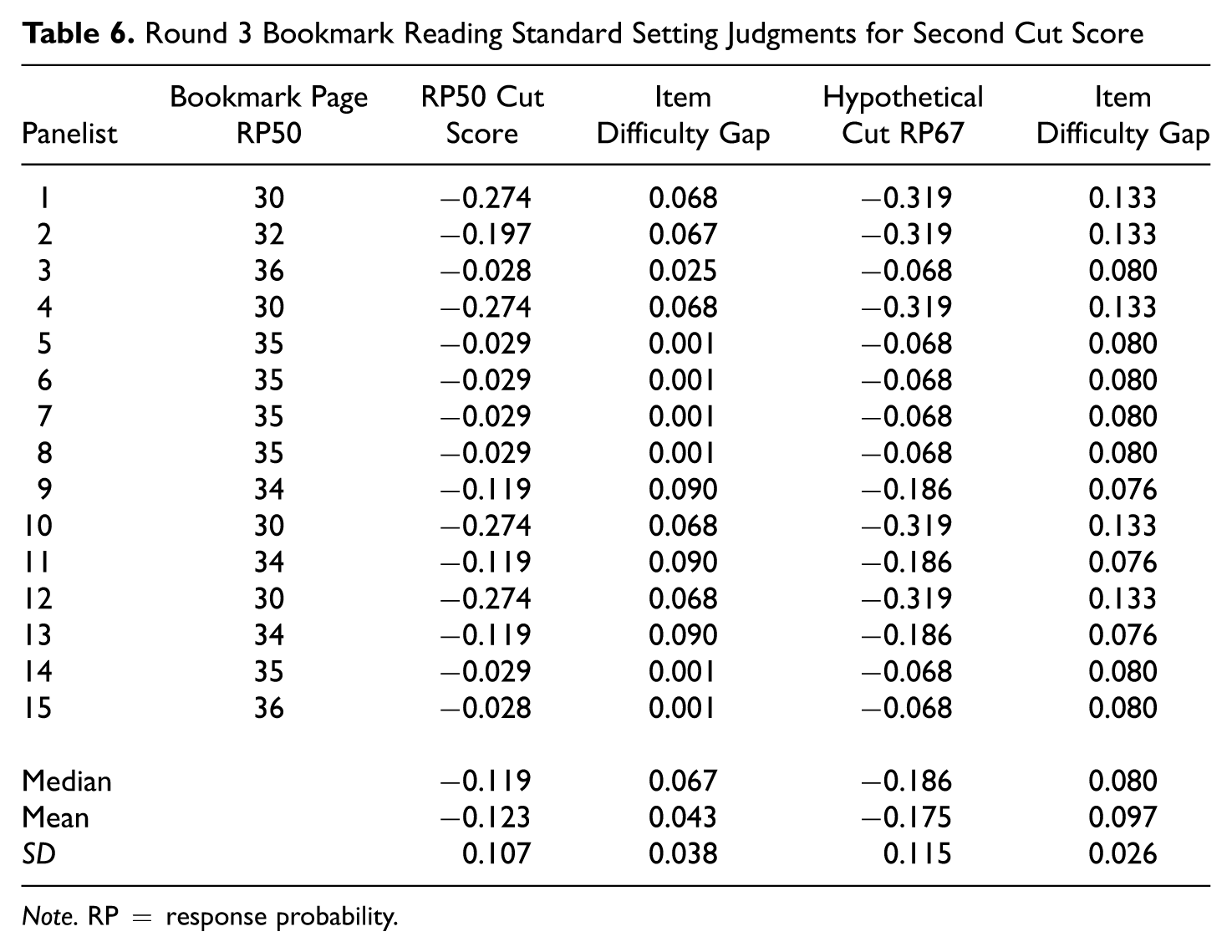
Note. RP = response probability.
Round 3 Bookmark Reading Standard Setting Judgments for Third Cut Score
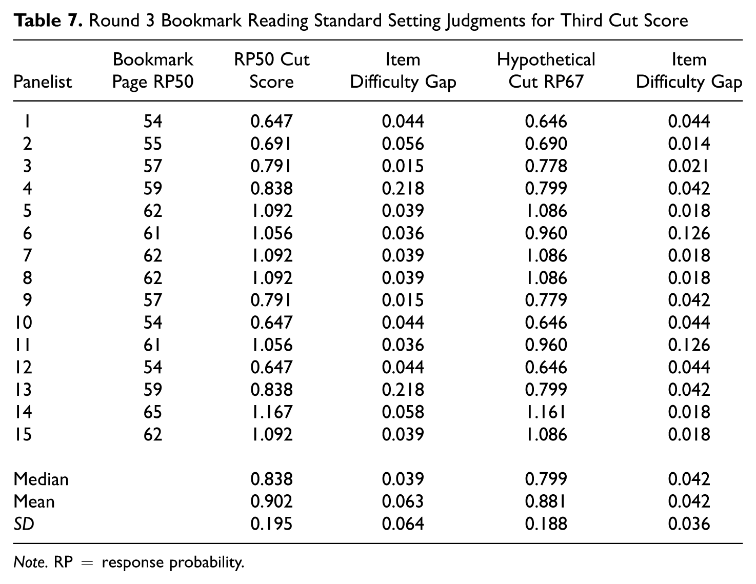
Note. RP = response probability.
Many of the patterns observed with the science assessments were again observed with the reading assessments. Most notably, the individual and group cut scores were again uniformly lower with RP67 compared with RP50. This again is opposite of what one might expect and is a function of the process that a panelist would use if they were employing the traditional Bookmark procedure to recommend cut scores with two different RP values. The mean, median, and standard deviation of item difficulty gaps and the panelist cut score estimates also show some of the variation in the cut scores that panelists recommended and the differences between cut score estimates when using the mean and median. For example, for the first cut score placement, the mean and median were −1.125 and −1.157 with RP50 compared with −1.136 and −1.206 with RP67.
The tables also suggest that there were the potential for some large item difficulty gaps near the locations of the cut scores. There was also the potential for large item difficulty gaps for the science assessments in Tables 3 and 4. Somewhat interestingly, the mean item difficulty gaps for some of the cut score recommendations were larger for some of the cut score placements for the reading assessments than the mean item difficulty gaps in the science assessments. This occurred despite the fact that the number of items used in the reading assessment example was twice the number used in the science assessment example. These data serve to illustrate that the potential for item difficulty gaps to impact cut scores is not necessarily isolated to a particular IRT model. They also suggest that simply increasing the numbers of items used in standard setting does not necessarily ensure that item difficulty gaps will be smaller and that cut scores when using different RP values will be more similar.
The tables also illustrate that even if there are small gaps under one RP value, there will not necessarily be small gaps under a different RP value with the 3PL model. For example, Panelist 11 has a relatively small item gap 0.004 for the panelist’s first cut score placement under RP50 on the reading assessment, but this value would be quite a bit larger at 0.703 with RP67. The panelist’s cut score also goes down by 0.304 in this case. Other differences between gaps and cut scores can be found in some of the other tables.
The PAC from the operational assessment can again be used to quantify the practical impact of the different RP values. For the first cut score, if median were used to compute the cut score, 0.17% more students would be at or above the cut score with RP67 compared with 0.74% more students being at or above the cut score when using the mean. For the second cut score, the differences are 2.03% and 1.41% more students being at or above the cut score with RP67 for the median and mean group cut scores, respectively. For the third cut score, the differences are 1.01% and 0.71% more students being at or above the cut score with RP67 for median and mean cut scores. With the expectation of the 0.00 difference in PAC for the second cut score based on the median for the science data, the differences for the reading data were smaller than those for the science data. This may be a function of the fact that the 3PL model has many more possible scores that are observed on the assessment, and it allows closer matching of estimated cut scores when computing the PAC. However, the observed differences with the reading data may be still of practical concern. For example, a potential one or two percent change in the PAC from using a different RP value is quite large given the stakes that are often attached to these cut scores. This magnitude of a potential change in the PAC is larger than one might expect.
Discussion and Conclusion
One persistent question in Bookmark standard setting is related to whether or not it is possible to end with the same cut scores with different RP values. The formulas and examples presented in this article show that it is theoretically possible to end up with the same cut scores with different RP values, but rarely is it possible to end up with the same cut scores in practice. This occurs because OIBs are not designed so that panelists could place their bookmarks to end up with the same cut score estimates because of the presence of item difficulty gaps. The appendix shows the formulas of items needed with the Rasch and 3PL models to end up with the same cut scores with two different RP values. The finding that it is not universally possible to obtain identical cut scores with different RP values unless the items have specific properties is a unique contribution of this study, which clarifies Hambleton and Pitoniak’s (2006) statement regarding when one should expect cut scores to be identical with different RP values.
This might lead one to suggest that OIBs should be designed so that cut scores under different RP values could turn out to be identical. However, this suggestion presents challenges in many practical situations. These challenges occur in practical situations because the restrictions that need to be satisfied to end up with the same cut scores under different RP values are hard to maintain. Specifically, there is typically only a fixed set of items from which one can design an OIB. In many circumstances, these items come from an intact test form that has been administered operationally. These items often do not have properties that would yield exactly the same cut scores under different RP values.
Moreover, the important concern in designing an OIB is with the item difficulty gaps between items where panelists intend to set their cut scores. If one just designed OIBs to end up with identical cut scores at different RP values, this might result in large item difficulty gaps between items. These gaps could create large potential biases in cut scores. As an extreme and purely hypothetical example, one could design two OIBs using the Rasch model where items were spaced at approximately 0.708 intervals so that the cut scores under RP50 and RP67 could be identical. This would create gaps of 0.708 units along the θ scale, which could potentially bias a panelist’s cut score by as much as 0.708.
Therefore, the important concern in designing an OIB is that the gaps in the regions where panelists intend to set their cut score are small. It is only when the items are well targeted to the desired cut score recommendations that the item difficulty gaps will be small and the cut scores will be well estimated. Ironically, even though it is easy to make this rather obvious point, it is impossible to know from the outset where panelists will set their cut scores. This means that in practice, all one can do is take the best guess at where one thinks the cut scores will be located and try to select items so that the gaps in these regions are small. This implies that it is not realistic to expect that OIBs can be designed to yield exactly the same cut score placements at all possible cut score locations with different RP values or that cut score would be identical if a different RP value was applied with the same items.
The empirical illustrations provided examples of what the impact of the item difficulty gaps could be on cut score estimates with RP50 and RP67 in a state testing program assuming that the same panelists applied the Bookmark procedure as it would be traditionally explained on the same set of items. It is important to recognize that the same group of panelists would typically not be asked to set cut scores with two different RP values. However, to answer the question of how close the cut scores could be if one used different RP values, one needs to make an assumption that the panelists are trying to set the same cut scores.
An important and somewhat unexpected finding from these examples was that if panelists applied the Bookmark procedure as is typically explained to attempt to match a previous cut score, cut score estimates would be lower with the second RP than with the first RP value. This is contrary to the Williams and Schulz (2005) study and the National Research Council report. The Williams and Schulz (2005) and the National Research Council (2005) studies differed from the current work in that panelists were not asked to set multiple cut scores where they conceptualized one RP value and then were asked to conceptualize another RP value. These studies used separate groups of panelists who conceptualized different RP values. These differences and other factors, such as the facilitators, the composition of the standard setting panels, or the specific implementations of the Bookmark procedure, could explain the differences between the hypothetical examples in this study and the findings presented in these operational situations. The important finding presented in this article is that differences in cut scores will undoubtedly be present if a different RP value was chosen with the same group of panelists. The cut scores would be expected to be lower with the second RP value no matter what the RP value.
Future research should investigate whether this theoretical finding holds in practice. In particular, an interesting future study would be to ask the same group of panelists to recommend two sets of cut scores on the same assessment conceptualizing different RP values. This would be very beneficial because it would provide essential insight into how panelists understand different RP values and the processes that panelists use to apply the Bookmark method with different RP values in practice. To date, a very limited amount of research has investigated the actual processes that panelists use in the Bookmark procedure or how they comprehend and use the RP criterion. Some of the qualitative research work by Hein and Skaggs (2009, 2010) is a notable exception. Research from Davis, Buckendahl, and Gerrow (in press) has also indirectly investigated this issue. They studied the impact of randomly ordering the OIB versus ordering the OIB correctly and found that cut scores were quite similar under both item orderings. They questioned some of the panelists’ perceptions when performing the Bookmark method in practice.
Deviations from the way that Bookmark procedure is typically designed to be implemented or their understanding of the RP criterion may mean that the theoretical results presented here may not necessarily hold in practice. The approach used in this article assumed that panelists understood the RP criterion and would apply Bookmark method with an alternate RP value in the way the Bookmark method is typically explained.
It is also important to point out that the differences that were observed in the cut scores with different RP values were function of the cut scores and the items that were used in the examples. Other assessments or group of panelists may yield different results from those in this article. These differences will occur in other situations since the characteristics of the OIBs and item difficulty gaps may be dissimilar and/or the panelists may choose to recommend different cut scores. The items and panelists’ cut scores that were used in this article were selected because they are representative of typical standard settings used in the state from which data came. Many other states use similar standard setting processes as those described in this article.
A key result from this research is that it extends the point made by Cizek and Bunch (2007) that when item difficulty gaps are present near where panelists want to set their cut scores, this can dramatically impact estimated cut scores. This research further indicates that item difficulty gaps can also affect the potential similarity of cut scores under different RP values and that the differences in cut scores with different RP values can translate into changes in the PAC that may have important practical impacts.
Footnotes
Appendix
The author declared no potential conflicts of interests with respect to the authorship and/or publication of this article.
The author received no financial support for the research and/or authorship of this article.