






Abstract
Multilevel structural equation modeling (MSEM) allows researchers to model latent factor structures at multiple levels simultaneously by decomposing within- and between-group variation. Yet the extent to which the sampling ratio (i.e., proportion of cases sampled from each group) influences the results of MSEM models remains unknown. This article explores how variation in the sampling ratio in MSEM affects the measurement of Level 2 (L2) latent constructs. Specifically, we investigated whether the sampling ratio is related to bias and variability in aggregated L2 construct measurement and estimation in the context of doubly latent MSEM models utilizing a two-step Monte Carlo simulation study. Findings suggest that while lower sampling ratios were related to increased bias, standard errors, and root mean square error, the overall size of these errors was negligible, making the doubly latent model an appealing choice for researchers. An applied example using empirical survey data is further provided to illustrate the application and interpretation of the model. We conclude by considering the implications of various sampling ratios on the design of MSEM studies, with a particular focus on educational research.
Keywords
Clustered data structures can present challenges for general linear models that assume independence of observations (Bentler & Chou, 1987; Raudenbush & Bryk, 2002). Yet clustered data structures can provide an opportunity for understanding how variables are related at more than one level. Multilevel modeling (MLM) adjusts for the violation of the homoskedasticity (or exogeneity) assumption of single-level linear regression, in which residual variance are no longer independent (Bentler & Chou, 1987; Rabe-Hesketh & Skrondal, 2008; Raudenbush & Bryk, 2002). MLM is frequently used to account for clustered data, where data are often clustered within higher level units, and thus continues to grow in popularity among applied researchers in the social and behavioral sciences (Raudenbush & Bryk, 2002; Snijders & Bosker, 1999). For instance, students may be clustered within schools, teachers may be clustered within districts, and individuals may be clustered within neighborhoods. By partitioning variation at different levels, multilevel modeling allows researchers to explore relationships among variables at two or more levels, and at the same time control for violations of independence that can have an adverse impact on the standard errors of model parameter estimates.
While observed variable multilevel analysis has a long-standing history in the social sciences, multilevel structural equation modeling (MSEM) continues to make substantial progress both in theory and application (see Hox & Maas, 2001; Jia & Konold, 2019; Muthén & Asparouhov, 2011; Preacher et al., 2010). MSEM is useful in accounting for measurement and/or sampling error, where Level 1 (L1) and Level 2 (L2) substantive latent constructs are estimated from a set of manifest observed variables. MSEM has spurred a number of theoretical and methodological research investigations that have focused on the performance of these models in applied settings. Some examples include estimating reliability of the L2 construct (Bliese, 2000), as well as formulating latent substantive constructs on the basis of latent-manifest variables (Lüdtke et al., 2011; Marsh et al., 2009).
One critical issue that has been underexamined in the MSEM literature is the sampling ratio. The sampling ratio represents the proportion of L1 cases sampled out of the total number of L1 cases within each L2 group that are potentially available. Often in educational and social sciences, researchers utilize cluster sampling designs to obtain a random sample of units from within each cluster, such as randomly sampling students in schools (Konold, 2018). Prior research by Lüdtke et al. (2008) and Marsh et al. (2009), for example, has explored measurement issues related to the sampling ratio in multilevel models, with focus on sampling error that arises when individual responses are aggregated to manifest L2 variables. Findings by Lüdtke et al. (2008) suggest that the sampling ratio may be related to bias in contextual effect estimates, in which an aggregated L2 variable has some effect on an outcome after controlling for L1 characteristics. This work was based on a formative aggregation process in which L1 units (e.g., individuals) respond to variables as they personally relate to themselves (e.g., I have been bullied this year). By contrast, reflective L2 constructs are measured through variables in which the referent is at L2 (e.g., ratings obtained by L1 students that are asked about the climate of their L2 school). Moreover, they focused on contextual effect estimates, in which aggregated group-level effects for an outcome are compared with individual-level effects. However, it has yet to be explored how sampling ratios are related to the measurement of L2 latent constructs themselves.
The overarching goal of this article is to more fully explore the sampling ratio in terms of how it is related to estimates of L2 factor loadings based on latent aggregations of L1 data. Toward that end, we build upon prior research by Lüdtke et al. (2008) who considered the role of the sampling ratio on sampling error in MSEM models. Specifically, we leverage previous research that has focused on L2 unreliability in contextual effect estimates due to sampling error, which includes both bias and efficiency. To address these gaps, we explored the role of the sampling ratio in MSEM models, by specifically examining the average relative bias and variability in estimates of L2 factor loadings through Monte Carlo simulations.
We begin by first considering how manifest multilevel models can be extended to MSEM for purposes of accounting for sampling error, measurement error, or both. Next, we discuss variability and reliability in MSEM models. We then distinguish between reflective and formative L2 constructs and consider theoretical and the modeling implications. Finally, we consider the interchangeability assumption and its relationship with the sampling ratio and the measurement of L2 latent constructs. After describing the setup of the simulation study, we summarize the various results. Last, we provide a general discussion of the findings, offering guidance for applied researchers, while also proposing future directions for additional research.
Multilevel Structural Equation Model Framework
The general MSEM framework proposed by Preacher et al. (2010) integrates confirmatory factor analysis (CFA)/structural equation modeling (SEM) and MLM into a single approach. A particular advantage of MSEM is that it decomposes observed individual ratings into two orthogonal L1 and L2 latent components, allowing for a more nuanced understanding and modeling of error sources. The terms latent components, latent constructs, and latent factors are used interchangeably throughout the text, and are akin to the concept of a latent trait in the context of item response theory (IRT) models. When evaluating L2 group effects through L1 responses, Lüdtke et al. (2011) argue that two types of unreliability may be present: measurement error in the indicators of L1 and L2 constructs, as well as sampling error due to the sampling of L1 individuals within each L2 group that are obtained for the purpose of responding to the manifest variables. They described a 2 × 2 taxonomy of ML models that account (or fail to account) for these different types of unreliability that may be present. We outline these four models below in relation to a two-level structure in which individuals (e.g., students) nested within groups (e.g., schools) respond to four manifest variables (e.g., individual students responding to four questions about the climate of their respective schools). Figure 1 provides a graphic representation of all four models.
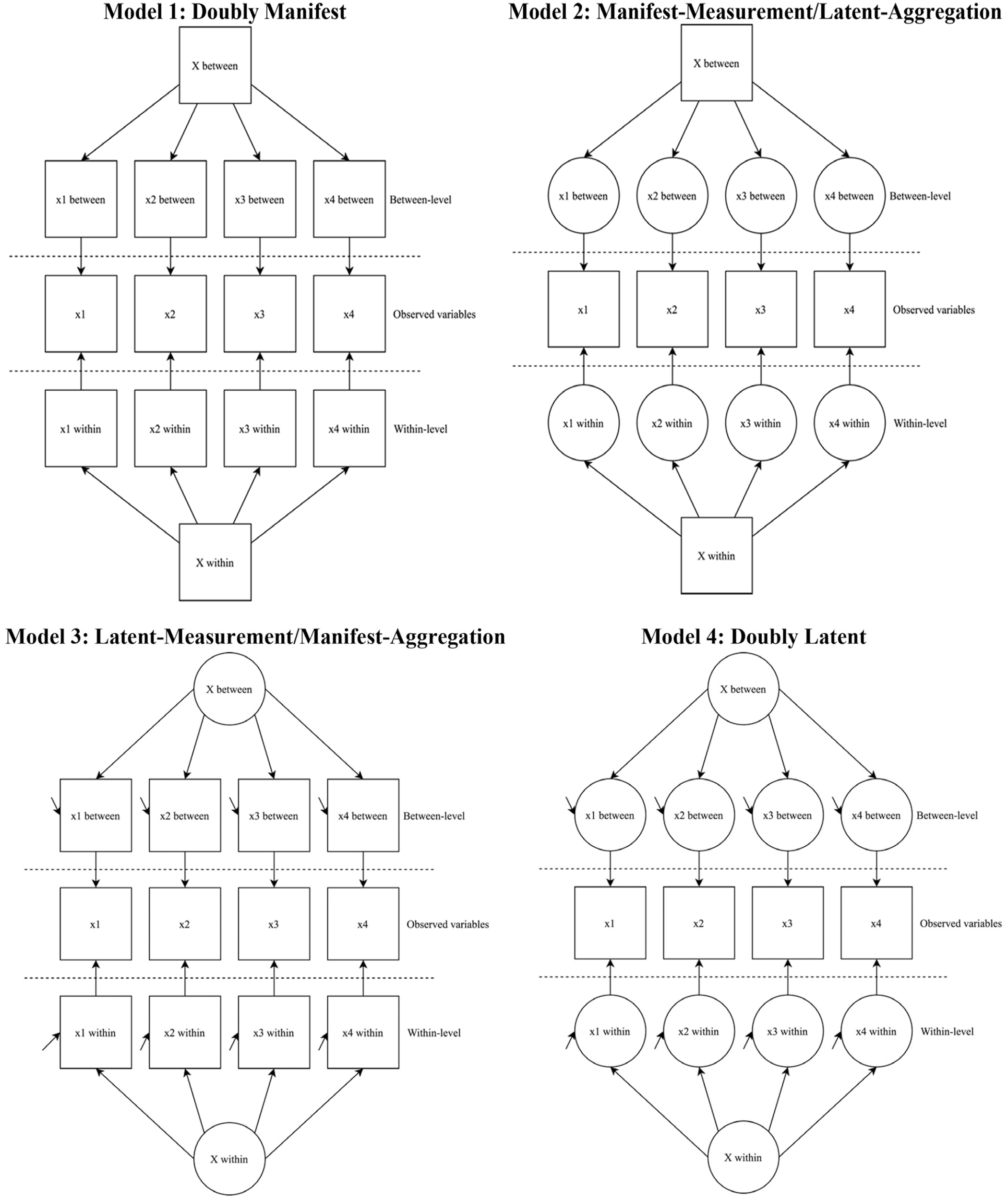
Graphic path diagrams of four MSEM measurement models. Circles represent latent variables; squares represent observed or manifest variables. Within and between levels are separated by a dashed line.
The doubly manifest model (Model 1) is the most basic model in that it assumes both measurement and sampling error are zero by failing to explicitly take these sources of variance into account. Here, the manifest observed variable is decomposed into two orthogonal L1 and L2 components. At the within-level, a single observed composite score
At the between-level, a single observed composite score
Model 1 in Figure 1 provides a graphic representation of this hypothetical model. This model is doubly manifest in that it combines observed variables to create a composite score (i.e., ignores measurement error) and that it uses a manifest aggregation from L1 to L2 (i.e., ignores sampling error). Moreover, this model “may be a highly unreliable measure of the unobserved group average” when a small number of L1 individuals are sampled from within each L2 group (Lüdtke et al., 2011, p. 450).
The issue of sampling error arises when individual responses are averaged within L2 units to compute an observed group-mean that is then used to represent L2 constructs (Nagengast & Marsh, 2011). Because L2 reflective traits are typically assessed through ratings obtained on a sample of L1 informants (e.g., students or teachers), different random samples may produce different estimates of the L2 trait. The sampling error inherent in a sample estimate like the mean can lead to bias in estimating substantive associations between L2 school climate constructs and other L2 outcomes (Shin & Raudenbush, 2010). This bias can become increasingly pronounced as the absolute size of the L1 units vary across L2 units. Here, greater weight is given to schools with a larger number of informants when ratings are aggregated across schools (Wang & Degol, 2016). According to Marsh et al. (2012), sampling error in L2 constructs obtained through aggregation of L1 response ratings are “a function of the average agreement among individuals in the same group and the number of sampled individuals in each group” (p. 111). When there is strong agreement on a large number of items among informants within the same school, estimates of sampling error will be smaller. Consequently, these L1 responses will provide better estimates of the L2 school trait being measured.
To help control for sampling error, the manifest-measurement/latent-aggregation model (Model 2) separates the manifest observed variable into two orthogonal latent components at L1 and L2 (B. O. Muthén, 1989, 1990, 1994) that are then aggregated to obtain the L1 and L2 substantive trait variables. However, this model is still manifest-measurement in that it assumes no measurement error through the aggregation of the indicators. In this model, each observed indicator variable is measured at the within level, and may be decomposed as the sum for each group plus an individual deviation from the group average (Asparouhov & Muthén, 2007a; L. K. Muthén & Muthén, 2017):
where
where
where
Figure 1 also represents a hypothetical latent-measurement/manifest-aggregation model (Model 3), with a single factor structure at both the within-level and between-level. This model can be conceived of as an extension of model 1 in that the L1 and L2 trait indicators are manifest, but substantive traits are formed as latent variables in a manner consistent with confirmatory factor analysis. This model accounts for measurement error in the indicators as the substantive trait factors represent shared variance across indicators, and residual sources of variance in the indicators modeled. The model is latent-measurement in that it takes into account measurement error at both L1 and L2 by estimating latent substantive factors that are measured by multiple L1 and L2 indicators. However, it is manifest-aggregation in that the observed group mean L2 indicators are the result of manifest aggregations from L1 to L2, thus not taking into account sampling error.
In the latent-measurement/manifest-aggregation model, the L2 latent factor
Letting
where
where
Model 4 in Figure 1 represents a hypothetical doubly latent model. This model builds on the latent-measurement/manifest-aggregation model (Model 3) by not only controlling for measurement error at L1 and L2 but also controlling for L2 sampling error through the latent L2 indicator aggregation process described for Model 2. In classical test theory, an individual’s observed score X is equal to the sum of the (unobserved) true score
while the between-level model is
Equations 8 and 9 may be combined into a single model:
In contrast to Model 3, the L2 indicator means are no longer manifest observed aggregations from L1, but rather are considered latent indicator variables with random intercepts. Thus, each observed indicator in the doubly latent approach is decomposed as is shown in Equations 8 and 9. Identification of this model may be achieved in multiple ways, depending on the central research question. For instance, to estimate the latent factor variance at both levels, the first factor loading at both levels may be fixed to one. Conversely, estimation of all factor loadings at both levels may be achieved by constraining the factor variance at both levels.
All four models can be understood in relation to their corrections for unreliability. Model 1 implicitly assumes there is no measurement error and no sampling error and is thus considered to be a no correction model. Models 2 and 3 both represent partial correction models, where Model 2 corrects for sampling error in the aggregation of an L1 construct to form an L2 construct, and Model 3 corrects for measurement error by using multiple observed indicators to estimate L1 and L2 constructs. The doubly latent model can be considered a full correction model, in that it simultaneously corrects for both measurement error and sampling error.
ICC and Reliability
A common measure to conceptualize variation in multilevel models is the intraclass correlation coefficient (ICC). Depending on the MSEM model, there may be both a latent factor ICC (
where
where n represents the average number of L1 units sampled from group j. The reliability of the aggregated L2 construct is sometimes referred to as ICC(2) in organizational psychological literature (Bliese, 2000). Thus, it can be seen that as the
In MSEM models with latent factors, the
Clearly, the
When an identical model structure is assumed at both the within and between levels, researchers may further calculate the
where
A second measurement issue concerns sampling errors that arise when averaging individual responses to form L2 constructs. Equations 8 and 9 provide the multilevel extension of classical test theory, in which an observed indicator at L1 is decomposed into two uncorrelated L1 and L2 latent variables, as well as separate error scores at each level. Consequently, reliability at L2 is defined by two kinds of error: (1) measurement error of
Construct Meaning and Implications
Group-level constructs are typically estimated through the collection of information on individuals within each group. In organizational psychology, for example, each individual’s rating of job satisfaction may be combined to form an overall group average of job satisfaction within a company. Early work by Cronbach (1976) highlighted potential problems and noteworthy methodological issues that may arise when obtaining group-level estimates through the aggregation of individual observed responses. One issue relates to the referent of L1 ratings, and the nature of the construct under study. Prior work by Lüdtke et al. (2008) and Stapleton et al. (2016), among others, distinguishes between formative and reflective L2 constructs, sometimes referred to in the literature as configural and shared constructs, respectively. The main distinction between the two constructs lies in the reference group, where the individual is the referent in the aggregation process for formative constructs, while the group itself is the referent in the aggregation process for reflective constructs. Moreover, prior research has established various recommendations regarding appropriate modeling of these differing constructs (Jak, 2019; Kim et al., 2016; Stapleton et al., 2016). These considerations are described in detail below.
Reflective Constructs
Consider a process in which student ratings of a common organizational trait like school safety are aggregated to form an overall school-level safety construct. This represents a reflective L2 aggregation process because each student is providing an estimate of a common trait. Observed indicators of reflective constructs are considered isomorphic across units within a given cluster, where responses to items are seen as interchangeable (or exchangeable), an important concept in multilevel modeling and organizational theory (Bliese, 2000; Bliese et al., 2007; Stapleton et al., 2016). Individuals within an L2 group may be considered interchangeable if their observed indicator responses all have the same relationship to the unobserved group mean
Furthermore, for reflective L2 constructs, the within-component is often not of interest, as there should in theory be no variability at L1 for a reflective construct. For reflective constructs, Stapleton et al. (2016) have proposed fitting a saturated model at the within-level for reflective constructs. However, Jak (2019) argues that the same result could be achieved by fitting a two-level factor model with factor loadings constrained to be equal across both levels, in which the variance of the L1 factor is assumed to be zero. Jak (2019) further demonstrates the two-level factor model with cross-level invariance to be less parameterized than the saturated model.
Reflective aggregations of L1 constructs may conflate multiple sources of variance, including variability associated with the measurement of the L2 construct, as well as residual variance unique to each individual (Marsh et al., 2012). Consider the example in which student ratings of school safety are aggregated to form an L2 overall school safety construct. It is likely that student ratings of school safety are influenced by both the student’s personal experiences of safety as well as their shared experiences and the perceptions generally held among his or her peers. Failing to disaggregate residual variance components in aggregated L2 constructs has been shown to introduce bias in estimates of L2 effects (Lüdtke et al., 2008; Morin et al., 2014).
Formative Constructs
Next, consider a process in which each student’s grade point average (GPA) is aggregated to form an overall school-level mean grade point average. This represents a formative L2 aggregation process because the measurement pertains to the student and there is no reason to believe all students should have the same GPA. In contrast to reflective L2 constructs, individuals within an L2 group are not considered to be interchangeable for formative L2 constructs. Rather, they are likely to have different (unique) L1 true scores because they are the referent of their own measurements, as the referent is the individual. More simply, the responses to L1 indicators are assumed to be influenced by the L1 construct (i.e., causal arrows in the structural model go from the L1 construct to the L1 indicators). As a result, there is no expectation that L1 variables and aggregated L2 variables represent the same construct. In contrast to the measurement of reflective constructs, when dealing with formative constructs, the latent factors at both L1 and L2 are often of substantive interest.
To appropriately model formative L2 constructs, researchers have suggested constraining factor loadings to be equal across levels, as the construct “reflects the cluster aggregate of the individual construct at Level 1” (Stapleton et al., 2016, p. 496). Here, cross-level invariance is necessary to establish construct validity of formative L2 constructs (Kim et al., 2016). Importantly, by imposing this cross-level invariance constraint on factor loadings, the covariance structure at L2 is identified, so long as the factor variance at L1 is constrained. As a result, other parameters may differ across levels, while the factor variance at L2 remains estimable (Jak, 2019).
The Role of the Sampling Ratio
Assumptions regarding the interchangeability of L1 individuals may have important implications regarding the reliability of L2 construct estimates. Examining Equation 12, it can be seen that reliability in the L2 construct estimates does not account for variation at L1. Instead, it is assumed that L2 unreliability due to sampling error is based on interchangeable individuals. As average group size (n) increases, all things equal, sampling distributions and standard errors decrease, while reliability increases (Jia & Konold, 2019). However, the relative size of the sample of L1 individuals from a population of potential L1 individuals within an L2 group can play a role when estimating aggregated L2 constructs. Prior simulation work by Lüdtke et al. (2008) examined the role of the sampling ratio in MSEM models with aggregated formative L2 constructs. The sampling ratio simply represents the proportion of sampled individuals from within a group:
where the sampling ratio for group j (
Some (e.g., Marsh et al., 2012) have argued that as the sampling ratio approaches 1.0, it is reasonable to assume no sampling error in the measurement of a L2 construct. Others (e.g., Shin & Raudenbush, 2010) have argued that if each cluster is assumed to be sampled from a larger population of clusters, it is appropriate to account for sampling error by treating the unobserved group means as a latent variable measured with some amount of precision (Asparouhov & Muthén, 2007a). However, the ability to control for sampling error, and thus improve reliability in L2 construct estimates, depends in part on the sampling ratio. As a result, different MSEM models may be better equipped than others to control for the sampling error, leading to more unbiased estimates.
Overall, questions remain about the role of the sampling ratio in MSEM. Much of the previous work on the sampling ratio has considered its impacts on (a) contextual effect estimates in the context of (b) measurement Models 1 and 2 in Figure 1 (i.e., doubly manifest and manifest-measurement/latent-aggregation models). However, the effects of the sampling ratio on estimates of L2 factor loadings remains unknown, specifically within a doubly latent MSEM modeling approach (Model 4 in Figure 1). The current study was designed to investigate whether the sampling ratio is related to bias and variability in aggregated formative L2 construct measurement and estimation in the context of doubly latent MSEM models.
Methods
Overview of the Analyses
We used Monte Carlo simulation to investigate bias and variability in estimates of factor loadings for aggregated formative L2 constructs across differing sampling ratios. It is assumed that the number of L1 units within each L2 group is a finite number (e.g., 100), and that each cluster is of equal size. A two-step procedure was used to generate populations with finite L1 sample sizes and a fixed number of L2 units. In the first step, clusters were generated to establish a population model with a finite sample size within each L2 group (e.g., J = 250 clusters with
Data Generation and Analysis
Mplus version 8.4 (L. K. Muthén & Muthén, 2017) was used to generate the data corresponding to the model presented in Equations 8 and 9, in which a single L1 latent construct is measured by four observed indicators at the within-level. At the between-level, a single L2 latent construct is measured by four latent aggregated group means corresponding to each indicator at L1. A graphic representation of this model is provided by Model 4 in Figure 1. Consistent with Jak (2019) and Stapleton et al. (2016), factor loadings were constrained to be equal across levels. For each replication, the associated population dataset was saved. Next, for each population dataset, a random sample of L1 units were drawn from each cluster according to a specified sampling ratio using R version 4.0.0 (R Core Team, 2020) and saved as an analytic dataset. Finally, each analytic sample dataset was then analyzed using an external Monte Carlo simulation study in Mplus. For identification purposes, the variance of the L1 factor was constrained (to 1) for the model fit to the analytic sample data. This resulted in a total of 17 parameters estimated: four factor loadings (cross-level invariance), four residual variances at L1, four intercepts at L2, one factor variance at L2, and four residual variances at L2. The MplusAutomation package (Hallquist & Wiley, 2018) in R was used extensively to facilitate conducting the simulations in Mplus. Annotated R code used for data generation and analysis is freely available at https://github.com/jmk7cj/Sampling-Ratio-for-MSEM. An example Mplus input file used to generate population data is also provided, along with an example Mplus input file used to analyze the analytic sample datasets.
Simulation Conditions
The following conditions were manipulated: the number of L2 groups (J = 50, 100, 500), the total number of L1 units per L2 cluster (
Values for the conditions considered were informed both by prior MSEM simulation research and previous applied education research. Previous research by Hox and Maas (2001) and Maas and Hox (2005) found cluster sizes less than 50 may lead to biased estimates in multilevel structural equation models. Hox and Maas (2001) argued that more than 100 L2 groups may be needed for unbiased estimates of a between-level model with low
The total number of L1 observations per L2 cluster were also informed by simulation work from Lüdtke et al. (2008), who considered 25, 100, and 500 L1 observations per L2 cluster. We wanted to extend the larger end of this condition to 1,000 to more closely replicate group sizes that may be encountered in secondary school educational research (e.g., high schools with 1,000 or more students). Regarding
Values for the standardized factor loadings were informed by prior MSEM simulation literature by Hox and Maas (2001), Kim et al. (2012), Lüdtke et al. (2008), and Lüdtke et al. (2011), where values ranged from 0.3 to 0.9. In practice, standardized factor loadings may be even less for MSEM models examining educational data (Jia & Konold, 2019; Morin et al., 2014). Some (e.g., Kline, 2011; Sun et al., 2011) consider standardized loadings ≥0.40 as necessary for establishing the validity and reliability of a single indicator. As a result, we chose two values, where standardized factor loadings of 0.5 and 0.8 represent low and high values. These values can be interpreted as reliability of a single indicator, where a value of 0.8 indicates that 0.82× 100 = 64% of the observed variance can be explained by the latent factor (Lüdtke et al., 2011). Moreover, it was assumed that the factor loadings were invariant across L1 and L2 (see the appendix [available online] for calculations of standardized factor loadings for generating data).
Last, we chose four values of the sampling ratio: 5%, 20%, 50%, and 80%. In the only other simulation study examining sampling ratios in MSEM models, Lüdtke et al. (2008) considered sampling ratios of .2, .5, .8, and 1.0. We were interested in extending this to scenarios in which the sampling ratio is even less than 20%. For example, consider a high school with 1,000 students (as described above), a scenario often faced by educational researchers. A sampling ratio of 5% would result in a sample of 50 students. Many applied educational examples deal with less than 50 units per L2 group sampled (Marsh et al., 2012). As a result, we believe a lower sampling ratio is important in understanding effects when dealing with L2 groups of larger sizes.
Evaluation Criteria
All models were estimated in Mplus using maximum likelihood parameter estimation with robust standard errors (MLR; L. K. Muthén & Muthén, 2017). We are most interested in model estimates of the four standardized factor loadings. We focus on factor loadings for three important reasons. First, as demonstrated in Equation 13, standardized factor loadings are directly related to the
where
To better understand which simulation conditions contributed to bias, parameter coverage, and RMSE, we conducted four-way factorial analysis of variance (ANOVA) tests, in which bias, parameter coverage, and RMSE were dependent variables, and each of the manipulated simulation conditions (L2 sample size, total L1 units per L2 cluster,
Results
Our three criteria for model evaluation (i.e., bias, parameter coverage, and RMSE) were calculated for each factor loading, then averaged across all four loadings. Estimates for the average relative percentage bias, average 95% parameter coverage, and average RMSE for the four factor loadings are provided in Tables 1 and 2. Several general findings emerged across all conditions. In general, the results appeared to improve (i.e., less bias, greater parameter coverage, and smaller RMSE) as either the number of clusters increased, the number of L1 units within each L2 cluster increased, or the sampling ratio increased. This suggests better measurement of the L2 latent factor as either the L1 or L2 sample size increase, or the sampling ratio increase. All models with the condition of N = 20 total L1 units within each L2 cluster and SR = .05 had convergence rates less than 50%. In these scenarios, only a single unit within each L2 cluster was sampled (i.e., 0.05 * 20), representing a singleton cluster. However, every other condition achieved 100% convergence across the 1,000 replications. A series of factorial ANOVA tests was used to further understand how the simulation facet conditions (i.e., L2 sample size, total L1 units per L2 cluster,
Average Relative Bias, Parameter Coverage, and RMSE (Root Mean Square Error) for Standardized Loading = 0.5.
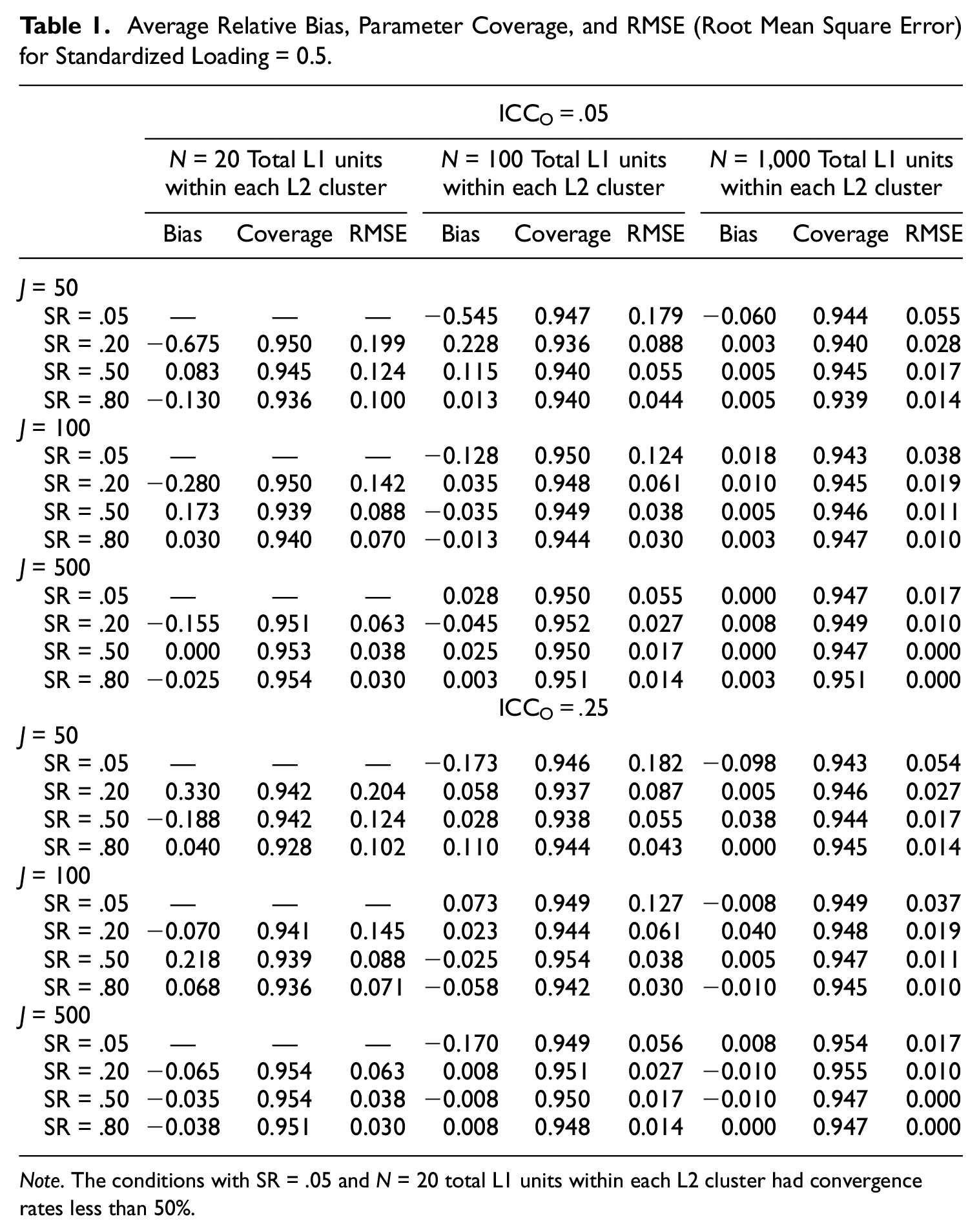
Note. The conditions with SR = .05 and N = 20 total L1 units within each L2 cluster had convergence rates less than 50%.
Average Relative Bias, Parameter Coverage, and RMSE (Root Mean Square Error) for Standardized Loading = 0.8.

Note. The conditions with SR = .05 and N = 20 total L1 units within each L2 cluster had convergence rates less than 50%.
Omega-Squared Values for Analysis of Variance Effects of Simulation Conditions.

Note. RMSE = root mean square error. Omega-squared effect sizes of small (
Bias
The relationship between certain facets and the relative percentage bias in parameter estimates are shown in Table 3. Main effect tests revealed that variations between L2 sample size, L1 sample size, and the sampling ratio resulted in meaningful (
To aid in interpretation of these findings, Figure 2 depicts the relationship between the relative percentage bias in estimates of the standardized factor loadings and the sampling ratio, with varying combinations of facets. Examining this figure, it can be seen that the largest values of bias occur for scenarios with a sampling ratio of 0.05. In fact, this sampling ratio of 5% is not plotted in the top panel, in which the total number of L1 units within each L2 cluster is 20, as these models failed to converge. However, it can be seen that bias decreases as the number of clusters increases, the number of L1 units within each L2 cluster increases, and the sampling ratio increases.
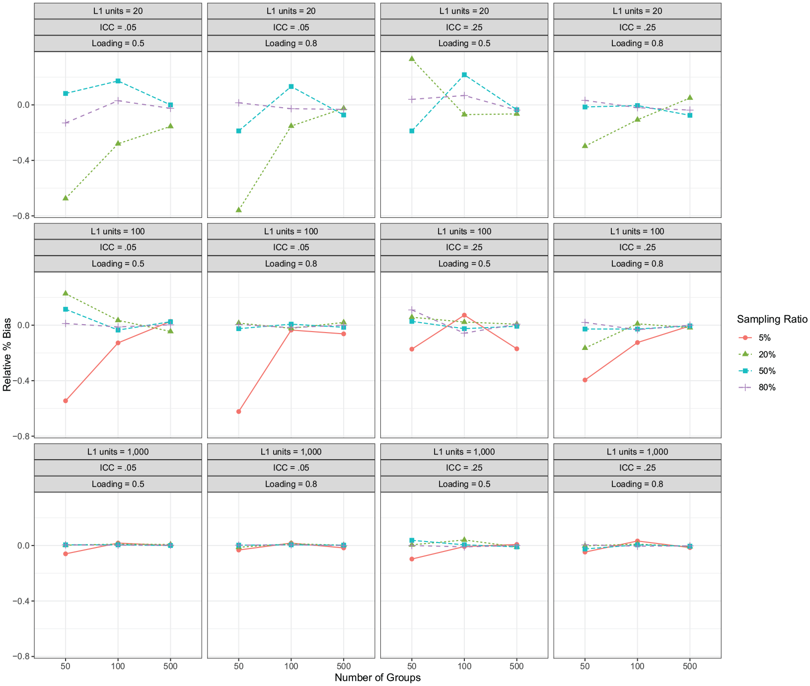
Relationship between the bias of estimates of the factor loadings and the sampling ratio, with varying combinations of facets.
While there appears to be considerable variability in bias across the simulation conditions, it is equally important to consider the size of that variability. Overall, values of relative percentage bias were well within the acceptable range of ±5%, with no values outside of ±1% (M = 0.03, SD = 0.14). This finding indicates virtually no bias in estimated factor loadings across the conditions, demonstrating a desirable property of maximum likelihood estimation of doubly latent MSEM models.
Parameter Coverage
Next, we considered the proportion of replications in which the 95% confidence interval contained the true population parameter, or parameter coverage. Similar to the results for bias, the main effect of the sampling ratio was related to coverage (
Figure 3 is provided to help interpret these findings, by depicting the relationship between the parameter coverage of estimates of the standardized factor loadings and the sampling ratio, with varying combinations of facets. Exploring this figure, it can be seen that parameter coverage improves toward the correct 0.95 level as the number of L2 clusters increases. Similarly, as the sampling ratio increases, parameter coverage tends to increase as well. Following the findings from Figure 3, scenarios in which the total number of L1 units within each L2 cluster is 20 and the sampling ratio is 0.05 are not provided in the top panel, as these models failed to converge.
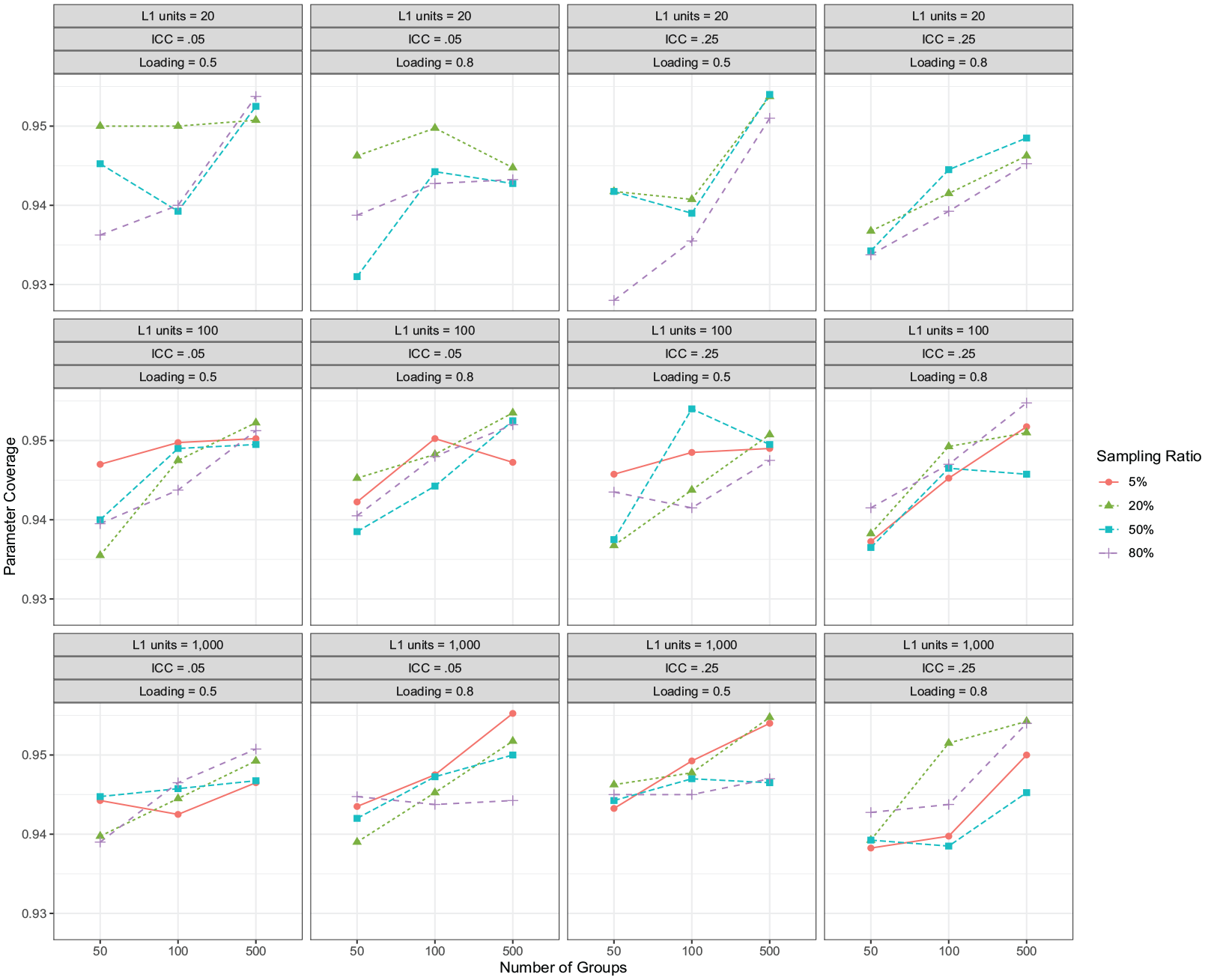
Relationship between the parameter coverage of estimates of the factor loadings and the sampling ratio, with varying combinations of facets.
Again, it is necessary to simultaneously consider the relative size of the variability of parameter coverage across simulation conditions. Overall, parameter coverage values were extremely close to the correct 0.95 value, with values ranging from 0.93 to 0.96 (M = 0.945, SD = 0.01). Thus, the standard errors for point estimates of factor loadings in doubly latent models demonstrate appropriate 95% confidence intervals almost perfectly match the appropriate 95% confidence intervals. While the sampling ratio is related to variability in parameter coverage across simulation conditions, the overall magnitude of these differences is essentially ignorable.
RMSE
An overall measure of accuracy was captured by calculating the RMSE. All main effects excluding the
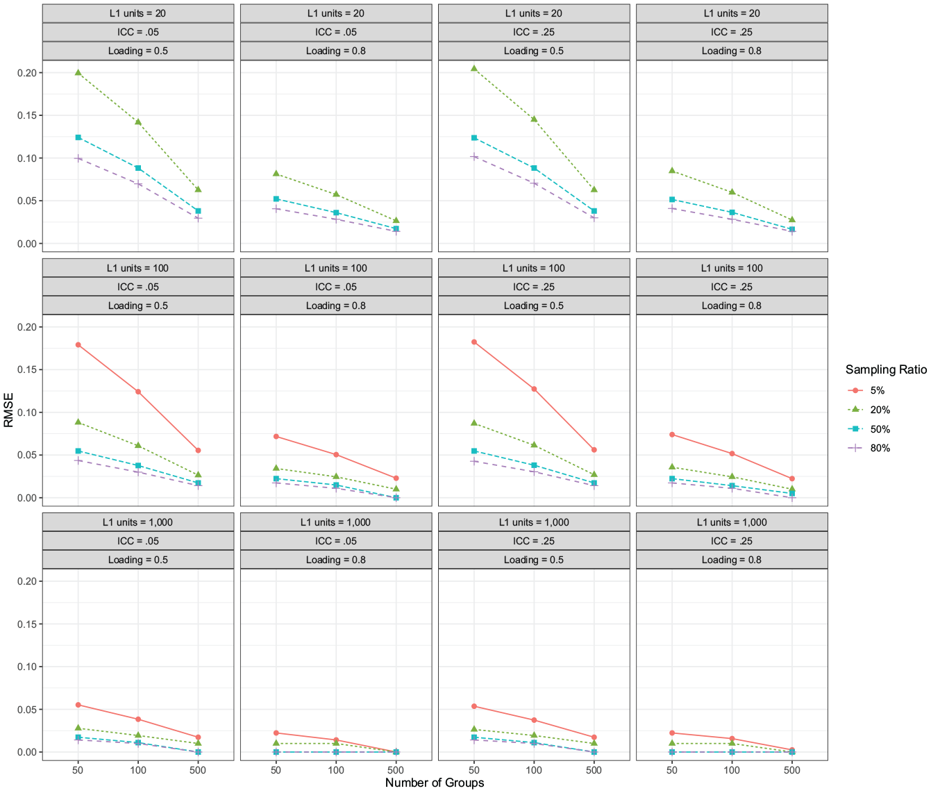
Relationship between the RMSE of estimates of the factor loadings and the sampling ratio, with varying combinations of facets.
Finally, although there is substantial variability in the RMSE of factor loading estimates, the overall size of that variability must also be considered. Examining Figure 4, it can be seen that RMSE values are relatively small, with all but one condition resulting in RMSE values below 0.20 (M = 0.04, SD = 0.04). Further analyses indicated RMSE nearly perfectly matched the parameter standard error (r = 0.997), where RMSE values were a function of the L1 sample size (Snijders & Bosker, 1993). These findings are consistent with doubly latent estimation reported by Lüdtke et al. (2011). As a result, although the variability in RMSE differs for various simulation facets, the maximum likelihood estimates produced by the doubly latent yielded reliably accurate results.
For Applied Researchers: Illustrative Example
In this section, we considered a case example using empirical survey data from the Early Childhood Longitudinal Study of Kindergarten (ECLS-K) study to illustrate the application and interpretation of doubly latent models. The ECLS-K study followed children from the kindergarten class of 1998-1099 through the spring of 8th grade in 2007, focusing on individual and school-level factors associated with early school experiences and performance (Tourangeau et al., 2009). For our example, we examined student achievement scores using public-release data in which students were nested within schools. While the original study involved a three-stage stratified sampling design, we assumed a simple random sample of schools and students within each school for simplicity. Additionally, listwise deletion was used to treat missing data. We restricted our sample to students with achievement scores measured in the spring of 5th grade (2004). This resulted in a sample of 10,447 students nested within 2,103 schools. The number of students sampled per school ranged from 1 to 34, with an average of 5 students per school. Moreover, based on school total enrollment, this resulted in a sampling ratio ranging from 0.13% to 18.7%, with an average sampling ratio of 3.7%. Thus, for example, if a school had a total enrollment of 500 students and 25 students were sampled, the sampling ratio was 5%.
We explored the possibility of a single latent factor at L1 (students) underlying three continuous variables representing student achievement scores in reading, math, and science, while also aggregating to a single latent factor at L2 (schools). This represents a formative L2 aggregation process as the measurement pertains to the student, and there is no reason to believe all students should have the same values for the three achievement variables. For formative constructs, students are not considered to be interchangeable, but rather are likely to have different, unique L1 true scores. In contrast to the measurement of reflective constructs (i.e., where the target of measurement is at a higher level), the latent factors at both L1 and L2 are often of substantive interest with formative constructs. Thus, a L1 indicator may represent a measure of student achievement, while a L2 indicator may represent the average student achievement within a school.
The three L1 achievement variables ranged from 0 to 96, in which reading (M = 50.28, SD = 10.13), math (M = 50.68, SD = 9.95), and science (M = 50.37, SD = 10.10) were all approximately normally distributed. Following the methods outlined in the simulation study, a doubly latent model with cross-level invariance was estimated in Mplus using maximum likelihood parameter estimation with robust standard errors. By fixing the L1 factor variance to one, a total of 13 parameters were estimated: three factor loadings (cross-level invariance), three residual variances at L1, three intercepts at L2, one factor variance at L2, and three residual variances at L2. We also estimated the model using the lavaan package (Rosseel, 2012) in R, although we do not report the results here as the output of the two programs was virtually identical. The dataset and annotated syntax for Mplus and lavaan are freely available at https://github.com/jmk7cj/Sampling-Ratio-for-MSEM.
Overall, the model fit the data well, with model fit statistics of comparative fit index = .997, Tucker-Lewis index = .991, root mean square error of approximation = .045, and standardized root mean square residual = .015. Estimated intraclass correlations at L1 for reading, math, and science achievement scores were 0.28, 0.26, and 0.35, respectively; values that are typical for educational achievement data in elementary school-aged students (Hedges & Hedberg, 2007). The
Table 4 presents the unstandardized parameter estimates. All three factor loadings were significantly related to students’ individual achievement at L1, as well as with average student achievement at L2, supporting the appropriateness of the measurement model. The estimated variance of the latent achievement factor at L2 was 0.56, while the variance of the latent achievement factor at L1 was constrained to one to allow for estimates of all factor loadings. However, imposing cross-level invariance ensures the latent factors are on a common scale, allowing for a direct comparison of latent factor variances across levels (Mehta & Neale, 2005). The proportion of variance explained by the latent achievement factor at L1 ranged from R2 = 0.64 to 0.68, while values at L2 ranged from R2 = 0.84 to 0.98.
Illustrative Example Results: Unstandardized Parameter Estimates of Student Achievement.
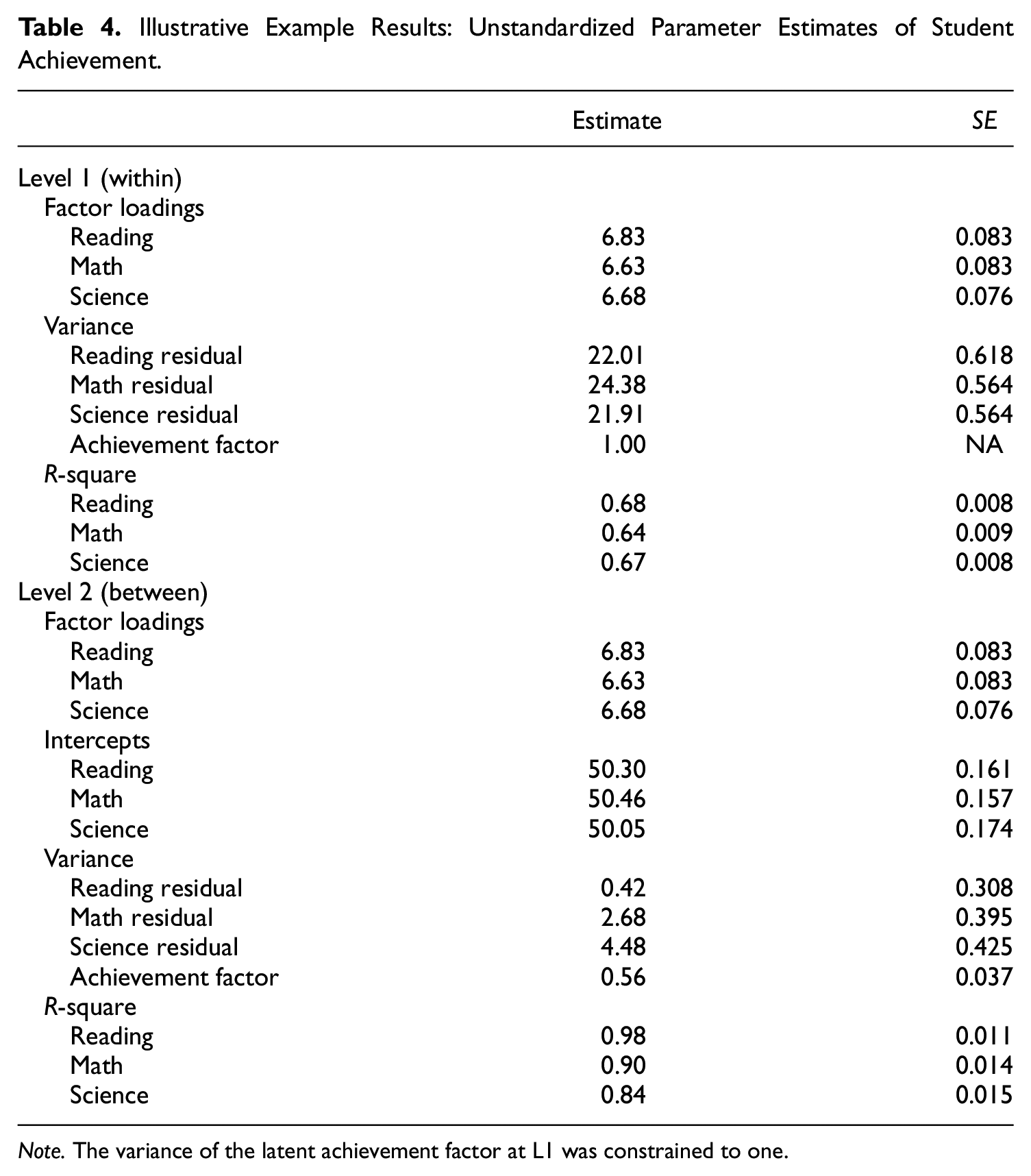
Note. The variance of the latent achievement factor at L1 was constrained to one.
Discussion
Multilevel models are often used by social science researchers to estimate effects of constructs at different levels on outcomes of interest. Various models have been proposed to control for measurement error and sampling error when measuring latent constructs at L2 through the aggregation of observed indicators at L1. Prior methodological and simulation research has developed the doubly latent approach that corrects for measurement error and sampling error, resulting in unbiased estimates of L2 constructs under certain conditions (Lüdtke et al., 2011; Marsh et al., 2009; B. O. Muthén, 1990). This present study adds to the literature by considering the role of the sampling ratio in doubly latent measurement models.
Our findings suggested that research designs utilizing the doubly latent model with low sampling ratios may face convergence problems. Similar problems with were demonstrated by Lüdtke et al. (2011) who found that doubly latent models often failed to converge for conditions with low
Results from the ANOVA indicated that as a main effect, lower sampling ratios also had negative effects on bias, coverage, and RMSE of estimated factor loadings. These findings appear to suggest that even after controlling for other design facets such as L1 and L2 sample size or
Among the various factors investigated in this study, we highlight the importance of the number of clusters sampled and the sampling ratio; these two factors are ones that researchers are likely to have the most control over, whereas it may be more difficult to control other facets such as the
In applied research studies, such as students nested within schools, the number of L1 units per cluster can vary considerably in size. For example, Larson et al. (2020) examined the effectiveness of classroom management practices on student engagement in secondary schools, in which N = 54 high schools ranged in total enrollment size from 323 students to 2,021 students. Consider an example research design in which a fixed sample of 50 students per school was collected. This could result in a sampling ratio ranging from approximately 2.5% to 15.5%, depending on the overall enrollment of the school. While findings from our simulation indicated that smaller sampling ratios (i.e., 5%) produced larger bias, worse parameter coverage, and larger RMSE, the overall size of these errors was essentially negligible. Thus, study designs with smaller sampling ratios of the type investigated here can be used to utilize doubly latent MSEM models for trustworthy results.
It is also important to note some software capabilities and limitations. For example, the doubly latent multilevel modeling approach, in which an individual’s observed score is simultaneously decomposed into two uncorrelated L1 and L2 latent variables plus separate error scores at each level, is the default setting in Mplus (Asparouhov & Muthén, 2007a; L. K. Muthén & Muthén, 2017). As first outlined by Lüdtke et al. (2011) and described in detail above, the doubly latent model is the only MSEM that corrects for both measurement error and sampling error. This is also the default estimation procedure for the lavaan package in R (Rosseel, 2012), which produced nearly identical parameter estimates and standard errors at both levels to those we obtained from Mplus. Likewise, the generalized linear latent and mixed model (gllamm) command in Stata 16 (Rabe-Hesketh et al., 2004; StataCorp, 2019) is also capable of estimating such models, while the gsem command is also capable in theory. However, more traditional multilevel software such as HLM 8 (Raudenbush et al., 2019) employ an observed variable disaggregation process to separate between- and within-group effects (Preacher et al., 2010), leading to an inability to estimate parameters and standard errors at each level simultaneously. In summary, the estimation techniques and capabilities of various software must always be considered by researchers and future studies.
Limitations and Future Directions
There are a number of limitations to our simulation study that should be considered, such as our use of multivariate normally distributed data. One assumption of maximum likelihood as a normal theory estimator is multivariate normality (Bollen, 1989). However, in educational and social sciences it is common for researchers to collect dichotomous and ordinal scale data. Different versions of weighted least squares estimators have been proposed to appropriately analyze multilevel models for categorical variables (Asparouhov & Muthén, 2007b; B. O. Muthén, 1984). However, all models in the current study used maximum likelihood parameter estimation with standard errors that are robust to nonnormality based on corrections by Yuan and Bentler (2000). While all of the indicators and latent factors at both levels were drawn from standard normal distributions in this study, MLR estimation in Mplus, as well as weighted least squares estimators, may protect against violations of multivariate normality. However, findings from this study should not be generalized to designs with dichotomous or count indicator variables. Instead, future researchers should consider the role of estimators specifically designed to handle categorical variables in MSEM and doubly latent models.
Second, the data generated for all conditions in our simulations were produced from a doubly latent true population model. Thus, the population model and the analytic model had the same factor structure at both levels and the same number of observed items at L1, albeit with differing sample sizes. However, it is possible and often useful to analyze data using different specifications than those used to generate the population model. Purposefully analyzing data with a model using the incorrect factor structure, using modeling approaches other than the doubly latent model, or selecting a sample of items from which to estimate factors may all be areas to investigate for future simulation research.
Third, the models we examined were assumed to represent formative L2 constructs, in which individuals within a L2 group were considered to be structurally different (and not interchangeable). At the same time, evaluating the sampling ratio for reflective L2 constructs may be impractical, as L1 units in this context are assumed to be interchangeable and thus have the same relationship to the unobserved group mean (Croon & van Veldhoven, 2007; Marsh et al., 2009). As a result, implications of the sampling ratio are most apt for formative L2 constructs.
Finally, we utilized a simple random sample of L1 units from each L2 cluster in our simulation study. As a result, for each replication, each unit within cluster j had a positive, equal probability of being selected for the analytic sample. However, it is possible to consider the effects of an unequal probability sampling design, in which the probability of being sampled is related to some known variable (e.g., only students with high test scores are sampled). Here, models would need to take into consideration the nonrandom differences among units and how these differences may be related to estimates of constructs of both L1 and L2. Again, future studies could construct an unequal probability sampling procedure relating to the sampling ratio to some other variable to investigate bias in parameter estimates. Furthermore, the use of quasi-experimental techniques (e.g., propensity scores) may play a role in balancing the covariate distribution, leading to improved estimates.
Conclusions and Implications
Multilevel structural equation modeling continues to make significant progress, with in-depth investigations of methodological techniques. The current study adds to the literature by exploring the role of the sampling ratio in MSEM models with a focus on the doubly latent model. The findings from our simulations indicated that while lower sampling ratios were related to increased bias, increased standard errors, and increased RMSE, the overall size of these errors was negligible, making the doubly latent model an appealing choice for researchers. The doubly latent model was originally proposed as an alternative to more simple ML models, with the ability to account for both sampling error and measurement error. Findings from our study demonstrated that estimation of L2 factor loadings in doubly latent models of formative L2 constructs produced accurate, reliable results across simulation conditions, even with varying sampling ratios, a property that researchers have long expected to be true. These findings have broad implications for educational, psychological, and social science research more generally, in which individuals are clustered within groups, and both L1 and L2 latent constructs are of interest. Future researchers are encouraged to utilize the doubly latent MSEM model for designs with smaller sampling ratios, as the model allows for the decomposition of a single indicator variable into within- and between-level specific components while correcting both sampling error and measurement error.
Supplemental Material
sj-pdf-1-epm-10.1177_00131644211020112 – Supplemental material for The Sampling Ratio in Multilevel Structural Equation Models: Considerations to Inform Study Design
Supplemental material, sj-pdf-1-epm-10.1177_00131644211020112 for The Sampling Ratio in Multilevel Structural Equation Models: Considerations to Inform Study Design by Joseph M. Kush, Timothy R. Konold and Catherine P. Bradshaw in Educational and Psychological Measurement
Footnotes
Acknowledgements
The authors would like to thank two reviewers whose suggestions substantially improved the manuscript. We also thank Jim Soland, Michael Hull, and Kelly Edwards for providing comments on an early draft of this paper.
Declaration of Conflicting Interests
The author(s) declared no potential conflicts of interest with respect to the research, authorship, and/or publication of this article.
Funding
The author(s) disclosed receipt of the following financial support for the research, authorship, and/or publication of this article: The research reported here was supported by the Institute of Education Sciences, U.S. Department of Education, through Grants R305H150027 and R305A150221 to the University of Virginia. The opinions expressed are those of the authors and do not represent views of the Institute or the U.S. Department of Education.

Supplemental Material
Supplemental material for this article is available online.
References
Supplementary Material
Please find the following supplemental material available below.
For Open Access articles published under a Creative Commons License, all supplemental material carries the same license as the article it is associated with.
For non-Open Access articles published, all supplemental material carries a non-exclusive license, and permission requests for re-use of supplemental material or any part of supplemental material shall be sent directly to the copyright owner as specified in the copyright notice associated with the article.
