Examining the Robustness of the Graded Response and 2-Parameter Logistic Models to Violations of Construct Normality

Abstract

When fitting unidimensional item response theory (IRT) models, the population distribution of the latent trait (θ) is often assumed to be normally distributed. However, some psychological theories would suggest a nonnormal θ. For example, some clinical traits (e.g., alcoholism, depression) are believed to follow a positively skewed distribution where the construct is low for most people, medium for some, and high for few. Failure to account for nonnormality may compromise the validity of inferences and conclusions. Although corrections have been developed to account for nonnormality, these methods can be computationally intensive and have not yet been widely adopted. Previous research has recommended implementing nonnormality corrections when θ is not “approximately normal.” This research focused on examining how far θ can deviate from normal before the normality assumption becomes untenable. Specifically, our goal was to identify the type(s) and degree(s) of nonnormality that result in unacceptable parameter recovery for the graded response model (GRM) and 2-parameter logistic model (2PLM).

Keywords

item response theory GRM 2PLM nonnormality simulation study parameter recovery

For unidimensional item response theory (IRT) models, the latent construct or trait (θ) is traditionally assumed to be normally distributed. The software programs used to fit unidimensional IRT models most commonly assume a normally distributed latent trait by default. However, there are situations where assuming or imposing a normal distribution may be inappropriate. One such situation is when a psychological theory posits that the latent construct is not normally distributed. As stated by Woods and Thissen (2006), not all theoretically expected population distributions for latent constructs can be reasonably approximated by a normal distribution. For example, constructs of a clinical nature, where symptoms tend to be low for most people, medium for some, and high for few, would not necessarily be expected to be normally distributed (see, for example, Reise & Waller, 2009). Additional constructs that are not likely to be normally distributed include self-esteem, borderline personality disorder, and dark triad traits (Reise et al., 2018).

Another situation where it may be inappropriate to assume or impose a normal distribution is when dealing with subsets of a population, or different populations generally. As an example, consider a researcher who was interested in examining item behavior on a scale in a sample drawn from a clinical inpatient population and a sample drawn from the general population. Realistically, there are many constructs that, if normally distributed in the general population, would not be expected to also be normally distributed in the inpatient subpopulation. It would be important to account for these different distributions as failure to consider a nonnormal latent construct could lead to mistaken conclusions regarding how a scale behaved in the two populations. Previous research has documented biased parameter estimates when the population distribution of θ is nonnormal and when program specifications restrict the shape of θ to normality. As stated by Woods (2007), assuming normality is a convenient choice but could severely alter the results of an analysis. Studies fitting a variety of IRT models exhibited decreased estimation accuracy when assuming normality under nonnormal conditions (Preston & Reise, 2013; Woods, 2006, 2007; Woods & Thissen, 2006). According to Woods and Thissen (2006), this bias increased as parameters became more extreme and as skew of the latent distribution increased.

If a researcher expects/desires the latent trait to be nonnormally distributed, there are methods available that account for nonnormality and do not carry the typical normality assumption. Techniques such as empirical histogram (EH; Mislevy, 1984; Woods, 2007) and Ramsay-curve IRT (RC-IRT; Woods, 2006; Woods & Thissen, 2006) simultaneously estimate the latent trait (θ) distribution and parameters within the expectation maximization (EM) algorithm of marginal maximum likelihood (MML-EM) estimation.

As described by Houts and Cai (2016), EH characterizes the shape of the latent trait distribution by using the normalized accumulated posterior densities for all response patterns at each quadrature point. Thus, the EH is derived based on the expected heights of each histogram bar. Woods (2007) outlined this process for estimating an EH as opposed to assuming that θ is normally distributed. Approximating the EH begins within the E-step of the EM algorithm. Based on the item parameters (treated as known) and θ (typically assumed to be normal), the frequency of endorsement for each response category is estimated at each quadrature point for every item. In each E-step, the estimated frequency distribution (similar to the one just described) from the prior E-step is used to define θ as opposed to the normal distribution. The rest of the algorithm proceeds as usual. This procedure allows for the item parameters and heights of the EH to be estimated simultaneously.

In contrast to EH, RC-IRT estimates the latent trait distribution as a smooth function and characterizes the shape of θ using a spline-based density-approximation procedure described by Ramsay (2000). In the E-step of the EM algorithm, the total number of respondents at each quadrature point is estimated using the current characterization of θ, which is assumed to be known. The normal distribution is used to start. In the M-step, after the likelihoods for each item are maximized, the likelihood of the current characterization of θ is maximized. The latent trait distribution is approximated as a Ramsay-curve through the use of basis spline (B-spline) functions. A combination of B-splines, that require the specification of the order of each B-spline polynomial function joined together at a specified number of knots, determine the shape of the Ramsay-curve. The order of the polynomial (i.e., degree) and the number of knots must be chosen by the researcher. These determine the number of B-splines (m) used during θ estimation and is formulated as

m = (d + 1) + n - 2

(1)

where n is the number of knots (points along θ where separate B-splines are joined together) and d is the degree of the polynomial.

Although these methods improve parameter estimates under nonnormal conditions, EH and RC-IRT come with an additional layer of complexity. When fitting models, characteristics of the latent trait distribution are now being estimated in addition to the item parameters. This can greatly increase computational burden and may lead to convergence issues. For example, when using EH, Woods (2007) observed a drop in convergence rates to under 100% for several conditions even when sample size was large (i.e., N = 1,000). In contrast, all conditions that assumed normality maintained 100% convergence regardless of the true shape of the latent trait distribution. Convergence rates of less than 100% have also been observed in simulation studies using RC-IRT when sample size was 1,000 (Woods, 2006; Woods & Thissen, 2006). However, these studies did not directly compare implementation of RC-IRT with conditions that assumed normality of θ. It seems that smaller sample sizes are likely to result in a greater proportion of nonconvergence. This would be problematic for psychological research that typically deals with sample sizes less than 1,000.

A study done by Shen et al. (2011) found a median sample size of 173 for studies published in Journal of Applied Psychology from 1995 to 2008. This is far less than the sample sizes used in previous simulation work that have demonstrated improved item parameter estimation accuracy when the latent trait distribution was freely estimated. Several studies found that nonnormality corrections improved estimation accuracy with sample sizes of 500 (Preston & Reise, 2013; Woods, 2006, 2007; Woods & Thissen, 2006), 1,000, and 2,000 (Preston & Reise, 2013). As smaller samples that reflect the approximate size found in Shen et al. (2011) were not examined, any adverse effects on parameter estimation are unknown and it is possible that implementing these nonnormality corrections when sample size falls below 500 is unlikely to lead to stable answers. However, this only becomes an issue if θ is not “approximately normal.” If the latent trait distribution happens to be “normal enough,” then it would be reasonable to use the simpler method of assuming normality (typically the program default). In such cases, the additional computational cost that comes along with nonnormality corrections is not worth the marginal improvement in estimation, assuming that there is an improvement at all.

It would be useful to further quantify the phrase “approximately normal.” As the computational burden of such corrections may prevent use in practice, it would be useful to further elaborate the limits of robustness to violations of this assumption. Our primary question of interest was as follows: How robust are estimates from a unidimensional IRT model that assumes θ is normal when θ is nonnormal? Because our focus is on the robustness to nonnormality, rather than correcting for it, we do not implement EH or RC-IRT in this study. Our first goal was to identify the most influential type(s) and degree(s) of nonnormality. Under the assumption of normality, we were interested in when parameter recovery becomes unacceptable. Our second goal was to provide recommendations for sample sizes that are common in psychological research. As the computational intensity of nonnormality corrections may cause issues with convergence, we were interested in assessing robustness to violations of the normality assumption, specifically in smaller sample sizes.

This study focused on the effect of nonnormality when fitting the unidimensional graded response model (GRM; Samejima, 1969) as well as the unidimensional 2-parameter logistic model (2PLM). The GRM is a common IRT model used in psychology and health assessment and the 2PLM represents a simpler case of the GRM. We use these models as a starting point for investigating the research questions posed in this study. The GRM is a polytomous IRT model for items with ordered categories (e.g., Likert-type rating scales). The GRM is mathematically defined as

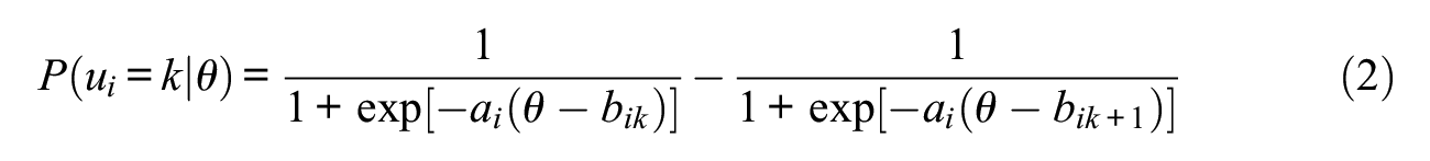
P (u_{i} = k | θ) = \frac{1}{1 + \exp [- a_{i} (θ - b_{ik})]} - \frac{1}{1 + \exp [- a_{i} (θ - b_{ik + 1})]}

(2)

This gives the probability of endorsing response option k given θ, which produces the observed response, u_i, to item i. The a-parameter represents the slope for item i and describes the relationship between an item and the latent trait. A higher slope indicates a stronger relationship between the item and the latent trait. The b-parameter represents the threshold of response option k for item i, where there are k−1 thresholds. If items have five response options, for example (and as is the case for the simulation in this study), there will be four thresholds. Threshold parameters convey information regarding the relative severity/difficulty of the available response options.

The 2PLM is a dichotomous IRT model for items with two response categories (e.g., yes vs. no, agree vs. disagree, and correct vs. incorrect). When there are only two response categories for an item, the GRM reduces to the 2PLM. The 2PLM is mathematically defined as

P (u_{i} = 1 | θ) = \frac{1}{1 + \exp [- a_{i} (θ - b_{i})]}

(3)

This gives the probability of endorsing an item i conditional on the level of the trait (θ). As with the GRM, the a-parameter for the 2PLM represents the slope for item i and describes the relationship between an item and the latent trait. The b-parameter represents the severity for item i and is the point on the latent trait continuum (θ) where there is a 50% chance of item endorsement (i.e., inflection point of the trace line). A higher severity/difficulty indicates that a greater amount of the latent trait is required to endorse the item.

In summary, this study sought to identify when nonnormality of the latent trait distribution (θ) is most impactful. Specifically, we assessed the effects of varying degrees of skew and kurtosis on estimation of the GRM and 2PLM when normality is assumed. The primary goal was to determine the robustness of these models to a nonnormal θ when normality is assumed.

Method

The shape of θ, sample size, and test length were manipulated. For the 2PLM, we also examined two different generating b-parameter distributions. Using Fleishman’s (1978) power method, the shape of θ was set to reflect distributions with varying types and varying degrees of nonnormality:

Y = e + fX + g X^{2} + h X^{3}

(4)

Using the polynomial displayed above, the power method transforms a standard normal variable (e.g., X) to a nonnormal variable (e.g., Y) that follows a population distribution (e.g., θ) with a target skew and kurtosis. For example, rounding to the hundredths place, substituting in the coefficients e = −0.112, f = 0.926, g = 0.112, and h = 0.198, will generate data that follow a population distribution with a skew of 0.75 and kurtosis of 1.30. A thorough review of approaches for generating nonnormal data, as well as a new approach for generating multivariate nonnormal data with a target skew and kurtosis, can be found in Qu et al. (2020).

For kurtosis, the values reported here are excess positive kurtosis. Although the kurtosis for a normal distribution is equal to 3, it is more common for software (and researchers) to report kurtosis minus 3 (i.e., excess kurtosis when compared with a normal distribution). We adapted and extended the skew and kurtosis values from Flora and Curran (2004) to create the distributional conditions in the current simulation. In Flora and Curran (2004), “low” and “moderate” skew were characterized by skew values of 0.75 and 1.25, respectively. “Low” and “moderate” kurtosis were characterized by kurtosis values of 1.75 and 3.75, respectively. To get a better sense of the effects of increasing skew and kurtosis, we added two levels of skew (1.75 and 2.25) and two levels of kurtosis (1.30 and 6.90).

When crossing skew and kurtosis levels, we did our best to maximize coverage of potential skew/kurtosis combinations while working within the constraints of Fleishman’s (1978) power method, which sometimes requires a specific level of kurtosis to achieve a target skew (e.g., minimum kurtosis of 1.30 required to achieve skew of 1.25). Finally, a standard normal distribution with no skew or kurtosis was included as a control condition. In summary, there were nine distributional conditions total, with five levels of kurtosis with skew constant at 0, three levels of skew with kurtosis constant at 1.30, and two levels of skew with kurtosis constant at 6.90 (Figure 1).

Figure 1.

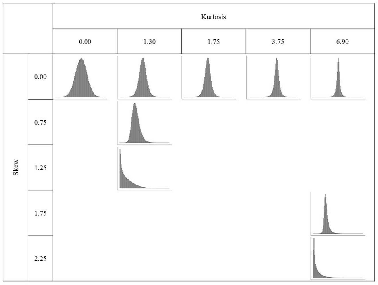
Skew and Kurtosis Combinations for Population Latent Trait Distribution (θ).

Samples of 125, 250, 500, and 1,000 were drawn from these population distributions. The first sample size of 125 was used to represent small samples that are common in psychological research (e.g., Shen et al., 2011). The other three sample sizes (250, 500, and 1,000) were used to mirror previous nonnormality work (Stone, 1992; Woods, 2006, 2007; Woods & Thissen, 2006). As in Stone (1992), test lengths were varied and set to 10, 20, or 40 items.

Item responses were generated under the GRM (five categories) or 2PLM (two categories). For the GRM, parameters were generated using the approach in Houts and Edwards (2013). Based on the a-parameter distribution documented in Hill (2004), a-parameters were drawn from a normal distribution with µ = 1.7 and σ = 0.3. Also from Hill (2004), b-parameters were generated by first drawing b₁ from a normal distribution with µ = −1.5 and σ = 0.5. Then, a difference parameter was drawn from a normal distribution with µ = 1 and σ = 0.2, and added to b₁ to create b₂ (see Woods, 2007). This process was repeated until a total of four b-parameters were created (b₂ = b₁+ difference parameter 1; b₃ = b₂+ difference parameter 2; b₄ = b₃+ difference parameter 3).

For the 2PLM, a-parameters were drawn from a normal distribution with µ = 1.19 and σ = 0.3. The generating distribution for b-parameters was an additional manipulation for the 2PLM. We were interested in the potential impact of different distributions on results and how results may need to be presented differently (conditionally or unconditionally) depending on this choice. This study examined two types of b-parameter distributions that are prevalent in the literature. Specifically, Stone (1992) randomly sampled b-parameters from a uniform distribution that ranged from −2.0 to 2.0. Alternatively, Woods and Thissen (2006) randomly sampled b-parameters from a normal distribution truncated at −2.0 and 2.0 with a µ = 0 and σ = 1. We slightly modified these distributions by extending the range (from −2.3 to 2.3).

The manipulated variables were fully crossed to create a total of 108 simulated conditions for the GRM (9 shapes of θ× 4 sample sizes × 3 test lengths) and an additional 216 simulated conditions for the 2PLM (9 shapes of θ× 4 sample sizes × 3 test lengths × 2 generating b-parameter distributions). Item responses were generated in R (R Core Team, 2020) with 1,000 data sets generated for each condition. Item parameters were estimated in flexMIRT (Cai, 2017) using MML-EM estimation. All program specifications were set to the defaults, which includes the assumption that θ is normally distributed. No additional postprocessing or parameter equating steps were conducted after estimation.

Mean absolute bias and root mean square error (RMSE) were computed as measures of parameter recovery.¹ Mean absolute bias was computed as the average absolute value of the difference between the estimated item parameters and the generated item parameters. For each parameter type, mean absolute bias and RMSE were averaged across items and replications. Values closer to 0 are indicative of better parameter recovery.

Cutoffs for what constituted acceptable recovery were determined by the conditions that satisfied the following Stone (1992) criteria (Table 1): Estimates of a-parameters were “generally precise and stable” when θ was normally distributed except for when N = 250 and test length = 10 (i.e., test length was at least 20) and estimates of b-parameters were “generally precise and stable” when N = 250 and test length = 10, even when θ had a positive skew of 0.75 (p. 12). For example, the GRM cutoffs in Table 1 for bias come from the Supplemental Table S1. For a-parameters, the cutoff was .16. This value corresponds to when θ is normal (skew = 0, kurtosis = 0), N = 250, and test length = 20 (Row 5, Column 4 of Supplemental Table S1), which is consistent with the a-parameter criteria described above. For b₁-b₄, the cutoffs are .16, .10, .11, and .17, respectively. These values correspond to when skew = 0.75, N = 250, and test length = 10 (Row 16, Columns 5–8 of Supplemental Table S1) and are consistent with the b-parameter criteria described above. Values of mean absolute bias and RMSE, when averaged across 1,000 replications for each condition, were considered acceptable if less than or equal to the respective cutoffs.

Table 1.

Cutoff Values for Acceptable Parameter Recovery Based on Stone (1992) Criteria.

Model	Parameter	Bias	RMSE
GRM	a	.16	.20
GRM	b ₁	.16	.20
GRM	b ₂	.10	.13
GRM	b ₃	.11	.14
GRM	b ₄	.17	.21
2PLM_TN	a	.19	.25
2PLM_TN	b	.20	.27
2PLM_U	a	.22	.28
2PLM_U	b	.27	.39

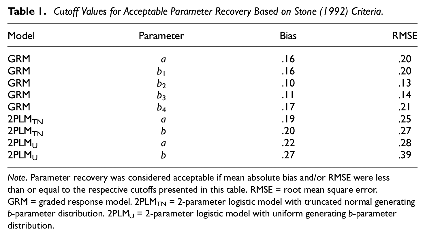
Note. Parameter recovery was considered acceptable if mean absolute bias and/or RMSE were less than or equal to the respective cutoffs presented in this table. RMSE = root mean square error. GRM = graded response model. 2PLM_TN = 2-parameter logistic model with truncated normal generating b-parameter distribution. 2PLM_U = 2-parameter logistic model with uniform generating b-parameter distribution.

Results

Convergence

Data sets were resampled and/or collapsed to encourage convergence and stable estimation. For the 2PLM, models were only fit to data sets with at least five simulees in each category for each item. As part of the data generation process, data sets were resampled if the number of simulees fell below five for any item category. For example, if data were being generated for a test with 10 dichotomous items, an item by category frequency table could be computed for each generated data set (20 cells in this case). If a generated data set resulted in at least one cell frequency less than five, then this data set would be discarded and resampled until a data set yielded cell frequencies that were all greater than or equal to five (i.e., at least five simulees for every item category).

For the GRM, categories with less than five simulees were first collapsed into an adjacent category. If the number of simulees was still less than five after collapsing, the data set would then be resampled (same procedure as used for the 2PLM). As expected, resampling was most prevalent with the smallest sample size of 125. A maximum of 92 data sets for a condition were resampled under the GRM, 34 under the 2PLM with a truncated normal generating b-parameter distribution (2PLM_TN), and 213 under the 2PLM with a uniform generating b-parameter distribution (2PLM_U). The rate of resampling was low for all other sample sizes, regardless of the shape of θ and test length. Data sets were rarely resampled when the sample size was 500 or 1,000 (96.3% of conditions did not resample and the remaining 3.7% only resampled once). When sample size was 250, the maximum number of resampling for a condition was 10.

Convergence was defined as a solution that met the first- and second-order tests in flexMIRT (Cai, 2017) as well as provided plausible estimates of parameters and corresponding standard errors.² The proportions of converged replications are displayed in Table 2. Aside from conditions with the most severe nonnormality (skew = 2.25 and kurtosis = 6.90), convergence for all GRM and 2PLM_TN conditions (normal and nonnormal θ) was high (above 95%) as long as sample size was greater than 125. Of note, none of the GRM conditions with N = 125 and test length = 40 converged and the GRM conditions with N = 125 and test length = 10 converged more than 95% of the time. Compared with the GRM and 2PLM_TN control conditions, the 2PLM_U condition with N = 250 and test length = 10 yielded convergence just below 95%. Convergence rates for all skewed 2PLM_U conditions with N = 250 fell below 95%. When θ was kurtotic and not skewed, an additional five out of 12 N = 250 conditions for the 2PLM_U fell below 95% convergence.

Table 2.

Proportion of Converged Replications.

Skew/Kurtosis	N	Test length	GRM	2PLM_TN	2PLM_U
0.00/0.00	125	10	0.999	0.863	0.701
0.00/0.00	125	20	0.936	0.889	0.719
0.00/0.00	125	40	0	0.754	0.383
0.00/0.00	250	10	0.999	0.987	0.949
0.00/0.00	250	20	1	0.988	0.962
0.00/0.00	250	40	0.997	0.977	0.965
0.00/0.00	500	10	1	0.999	0.996
0.00/0.00	500	20	0.999	0.995	0.994
0.00/0.00	500	40	0.999	0.992	0.992
0.00/0.00	1,000	10	1	1	0.997
0.00/0.00	1,000	20	1	0.999	1
0.00/0.00	1,000	40	0.997	0.995	0.998
0.75/1.30	125	10	0.993	0.843	0.643
0.75/1.30	125	20	0.904	0.864	0.640
0.75/1.30	125	40	0	0.695	0.306
0.75/1.30	250	10	1	0.981	0.938
0.75/1.30	250	20	0.999	0.988	0.950
0.75/1.30	250	40	0.993	0.969	0.935
0.75/1.30	500	10	0.997	0.996	0.994
0.75/1.30	500	20	1	0.999	0.994
0.75/1.30	500	40	0.999	0.999	0.992
0.75/1.30	1,000	10	1	1	0.999
0.75/1.30	1,000	20	1	0.999	0.999
0.75/1.30	1,000	40	0.999	0.999	0.999
1.25/1.30	125	10	0.989	0.797	0.572
1.25/1.30	125	20	0.877	0.822	0.481
1.25/1.30	125	40	0	0.599	0.194
1.25/1.30	250	10	1	0.959	0.840
1.25/1.30	250	20	0.998	0.975	0.872
1.25/1.30	250	40	0.991	0.970	0.875
1.25/1.30	500	10	1	0.996	0.978
1.25/1.30	500	20	1	0.997	0.990
1.25/1.30	500	40	1	0.993	0.994
1.25/1.30	1,000	10	0.998	0.997	0.992
1.25/1.30	1,000	20	0.999	0.999	0.998
1.25/1.30	1,000	40	1	0.997	0.997
1.75/6.90	125	10	0.990	0.785	0.529
1.75/6.90	125	20	0.819	0.800	0.486
1.75/6.90	125	40	0	0.545	0.186
1.75/6.90	250	10	1	0.957	0.879
1.75/6.90	250	20	0.996	0.966	0.919
1.75/6.90	250	40	0.978	0.962	0.865
1.75/6.90	500	10	1	0.992	0.987
1.75/6.90	500	20	0.999	0.996	0.994
1.75/6.90	500	40	0.998	0.995	0.983
1.75/6.90	1,000	10	0.999	0.999	0.996
1.75/6.90	1,000	20	0.999	0.999	0.997
1.75/6.90	1,000	40	0.998	0.998	1
2.25/6.90	125	10	0.973	0.703	0.392
2.25/6.90	125	20	0.639	0.644	0.293
2.25/6.90	125	40	0	0.345	0.050
2.25/6.90	250	10	0.999	0.910	0.720
2.25/6.90	250	20	0.996	0.927	0.664
2.25/6.90	250	40	0.945	0.901	0.582
2.25/6.90	500	10	0.999	0.974	0.906
2.25/6.90	500	20	0.999	0.992	0.940
2.25/6.90	500	40	0.998	0.986	0.931
2.25/6.90	1,000	10	1	0.995	0.971
2.25/6.90	1,000	20	0.999	0.996	0.992
2.25/6.90	1,000	40	1	0.996	0.996
0.00/1.30	125	10	0.996	0.875	0.666
0.00/1.30	125	20	0.926	0.863	0.703
0.00/1.30	125	40	0	0.718	0.343
0.00/1.30	250	10	1	0.980	0.959
0.00/1.30	250	20	0.996	0.991	0.970
0.00/1.30	250	40	0.994	0.979	0.959
0.00/1.30	500	10	1	0.998	0.993
0.00/1.30	500	20	1	0.992	0.996
0.00/1.30	500	40	0.999	0.991	0.989
0.00/1.30	1,000	10	1	0.999	1
0.00/1.30	1,000	20	0.999	0.999	1
0.00/1.30	1,000	40	0.999	0.997	0.997
0.00/1.75	125	10	0.995	0.843	0.677
0.00/1.75	125	20	0.913	0.876	0.674
0.00/1.75	125	40	0	0.694	0.347
0.00/1.75	250	10	0.999	0.990	0.951
0.00/1.75	250	20	0.998	0.984	0.967
0.00/1.75	250	40	0.994	0.978	0.947
0.00/1.75	500	10	1	0.999	0.993
0.00/1.75	500	20	1	0.997	0.992
0.00/1.75	500	40	0.999	0.998	0.993
0.00/1.75	1,000	10	0.999	1	1
0.00/1.75	1,000	20	1	0.997	0.998
0.00/1.75	1,000	40	0.999	0.999	0.998
0.00/3.75	125	10	0.989	0.843	0.653
0.00/3.75	125	20	0.881	0.850	0.676
0.00/3.75	125	40	0	0.692	0.327
0.00/3.75	250	10	0.999	0.985	0.929
0.00/3.75	250	20	0.998	0.986	0.964
0.00/3.75	250	40	0.991	0.968	0.945
0.00/3.75	500	10	1	0.999	0.988
0.00/3.75	500	20	0.999	0.997	0.999
0.00/3.75	500	40	0.998	0.998	0.992
0.00/3.75	1,000	10	0.999	0.999	0.999
0.00/3.75	1,000	20	0.999	0.998	1
0.00/3.75	1,000	40	0.998	0.999	0.997
0.00/6.90	125	10	0.988	0.825	0.622
0.00/6.90	125	20	0.847	0.826	0.657
0.00/6.90	125	40	0	0.659	0.297
0.00/6.90	250	10	0.999	0.974	0.921
0.00/6.90	250	20	0.998	0.979	0.958
0.00/6.90	250	40	0.980	0.963	0.929
0.00/6.90	500	10	1	0.998	0.987
0.00/6.90	500	20	0.998	0.999	0.994
0.00/6.90	500	40	0.997	0.991	0.993
0.00/6.90	1,000	10	1	0.999	1
0.00/6.90	1,000	20	0.998	1	0.998
0.00/6.90	1,000	40	0.999	0.999	0.996

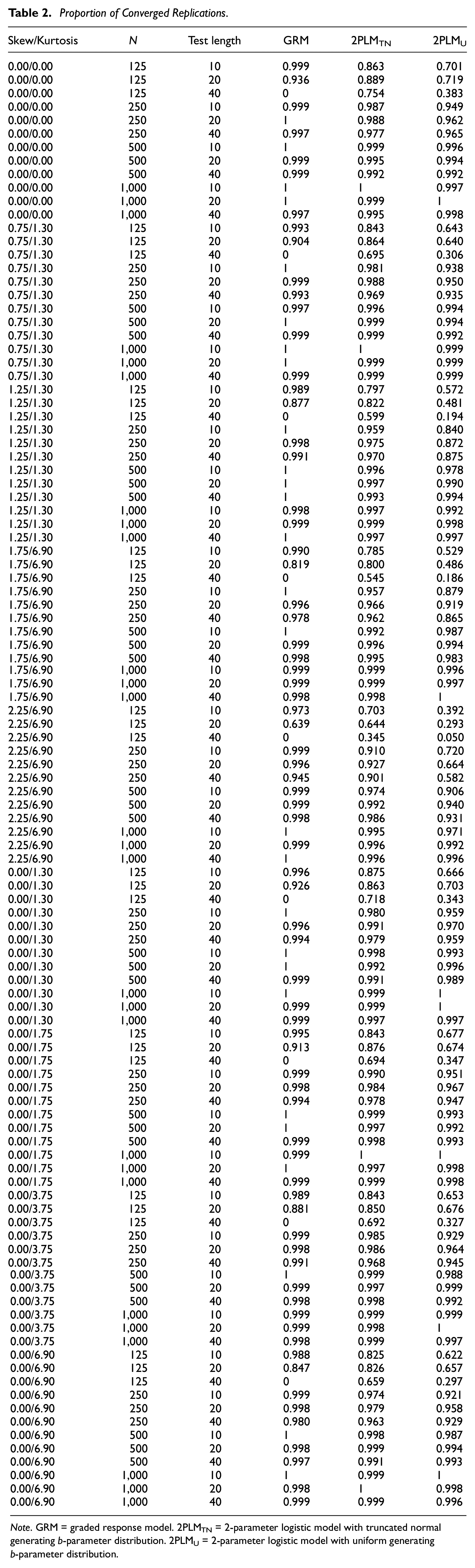
Note. GRM = graded response model. 2PLM_TN = 2-parameter logistic model with truncated normal generating b-parameter distribution. 2PLM_U = 2-parameter logistic model with uniform generating b-parameter distribution.

On average, conditions with the most severe nonnormality (skew = 2.25 and kurtosis = 6.90) led to the lowest convergence rates. For the GRM, the test lengths of 20 and 40 with a sample size of 125 fell below a 95% convergence rate. In addition, the test length of 40 with the sample size of 250 fell just below 95%. Under the most severe skew and kurtosis, all N = 125 and N = 250 conditions for the 2PLM_TN and all N = 125, N = 250, and N = 500 conditions for the 2PLM_U had convergence rates below 95% convergence.

Effects on Parameter Recovery

First, analyses of variance (ANOVAs) were run to assess which simulation variables (e.g., shape of θ, sample size, and test length) had the greatest impact on recovery of a-parameters and b-parameters (b₁-b₄ for the GRM). Effect sizes ( $η_{p}^{2}$ s) for GRM and 2PLM recovery measures are presented in Tables 3 and 4, respectively. On average for the GRM, mean absolute bias and RMSE were most influenced by sample size. Effect sizes ranged from .24 to .51 for all parameters. The second largest effect was the shape of θ. Effect sizes ranged from .10 to .19 for a, b₁, and b₄ (effects for b₂ and b₃ were negligible; $η_{p}^{2}$ s ≤ .07). For conditions included in the analysis, the effect of test length on GRM recovery measures was negligible ( $η_{p}^{2}$ s ≤ .03). For the 2PLM, across both types of generating b-parameter distributions, the order of effects mirrored the GRM. Mean absolute bias and RMSE were most influenced by sample size with effect sizes ranging from .24 to .61 for both a- and b-parameters. The next largest effect was the shape of θ with effect sizes ranging from .17 to .36 for both a- and b-parameters. The smallest effect, on average, was that of test length with effect sizes ranging from .14 to .20 for a-parameters only. The effect of test length on b-parameters was negligible ( $η_{p}^{2}$ s ≤ .06).

Table 3.

Effects on GRM Parameter Recovery Measures.

Variable	Parameter	$η_{p}^{2}$ _Bias	$η_{p}^{2}$ _RMSE
Shape of θ	a	.19	.17
	b ₁	.16	.17
	b ₂	.03	.03
	b ₃	.07	.06
	b ₄	.12	.10
Sample size	a	.45	.51
	b ₁	.26	.28
	b ₂	.24	.24
	b ₃	.24	.25
	b ₄	.24	.28
Test length	a	.03	.02
	b ₁	.02	.01
	b ₂	<.01	<.01
	b ₃	<.01	<.01
	b ₄	<.01	<.01

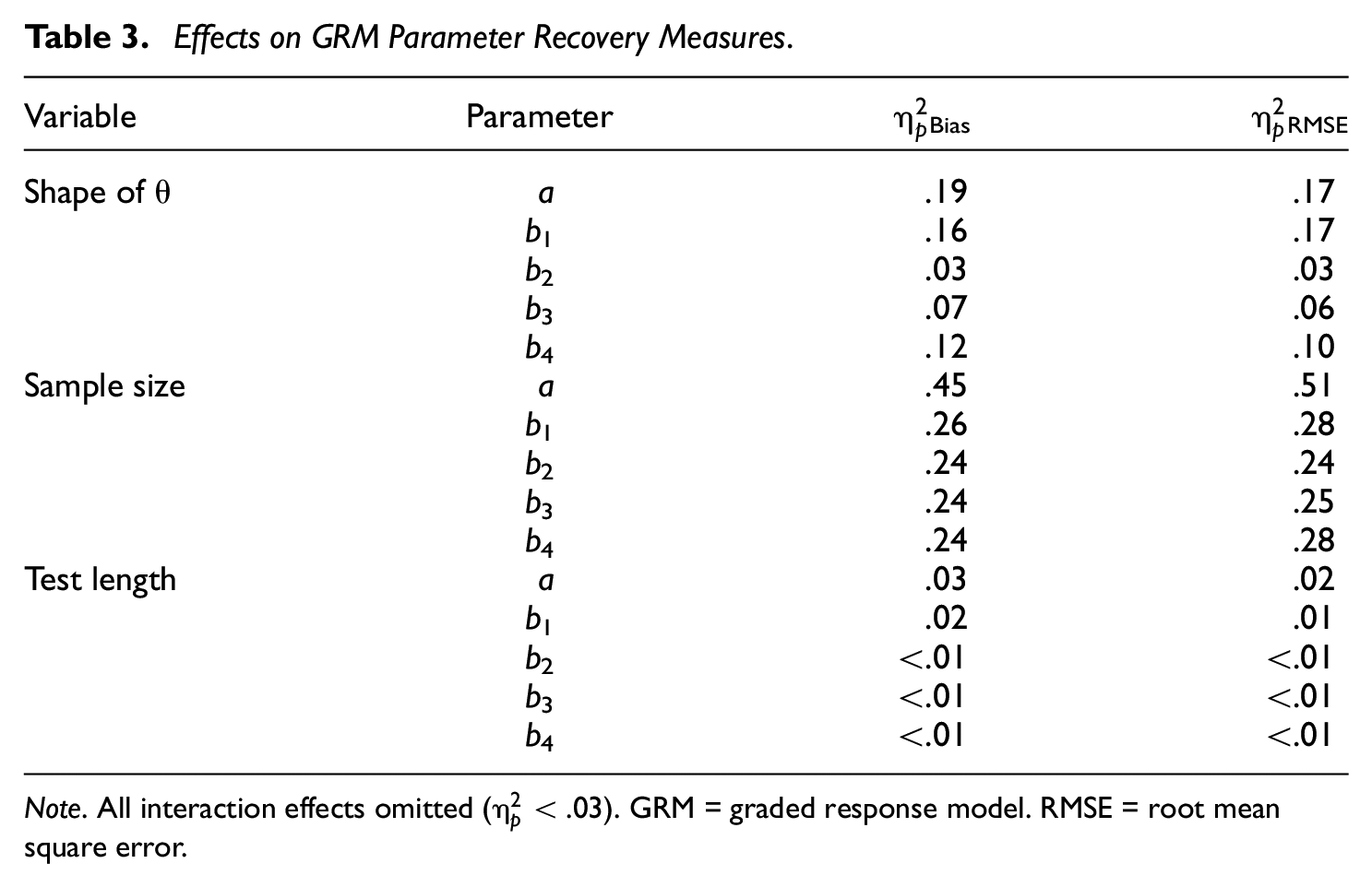
Note. All interaction effects omitted ( $η_{p}^{2}$ < .03). GRM = graded response model. RMSE = root mean square error.

Table 4.

Effects on 2PLM Parameter Recovery Measures.

Truncated normal generating b-parameter distribution
Variable	Parameter	$η_{p}^{2}$ _Bias	$η_{p}^{2}$ _RMSE
Shape of θ	a	.26	.23
Shape of θ	b	.20	.17
Sample size	a	.61	.59
Sample size	b	.43	.31
Test length	a	.17	.14
Test length	b	.04	.02
Uniform generating b-parameter distribution
Variable	Parameter	$η_{p}^{2}$ _Bias	$η_{p}^{2}$ _RMSE
Shape of θ	a	.36	.32
Shape of θ	b	.32	.31
Sample size	a	.55	.52
Sample size	b	.32	.24
Test length	a	.20	.16
Test length	b	.06	.03

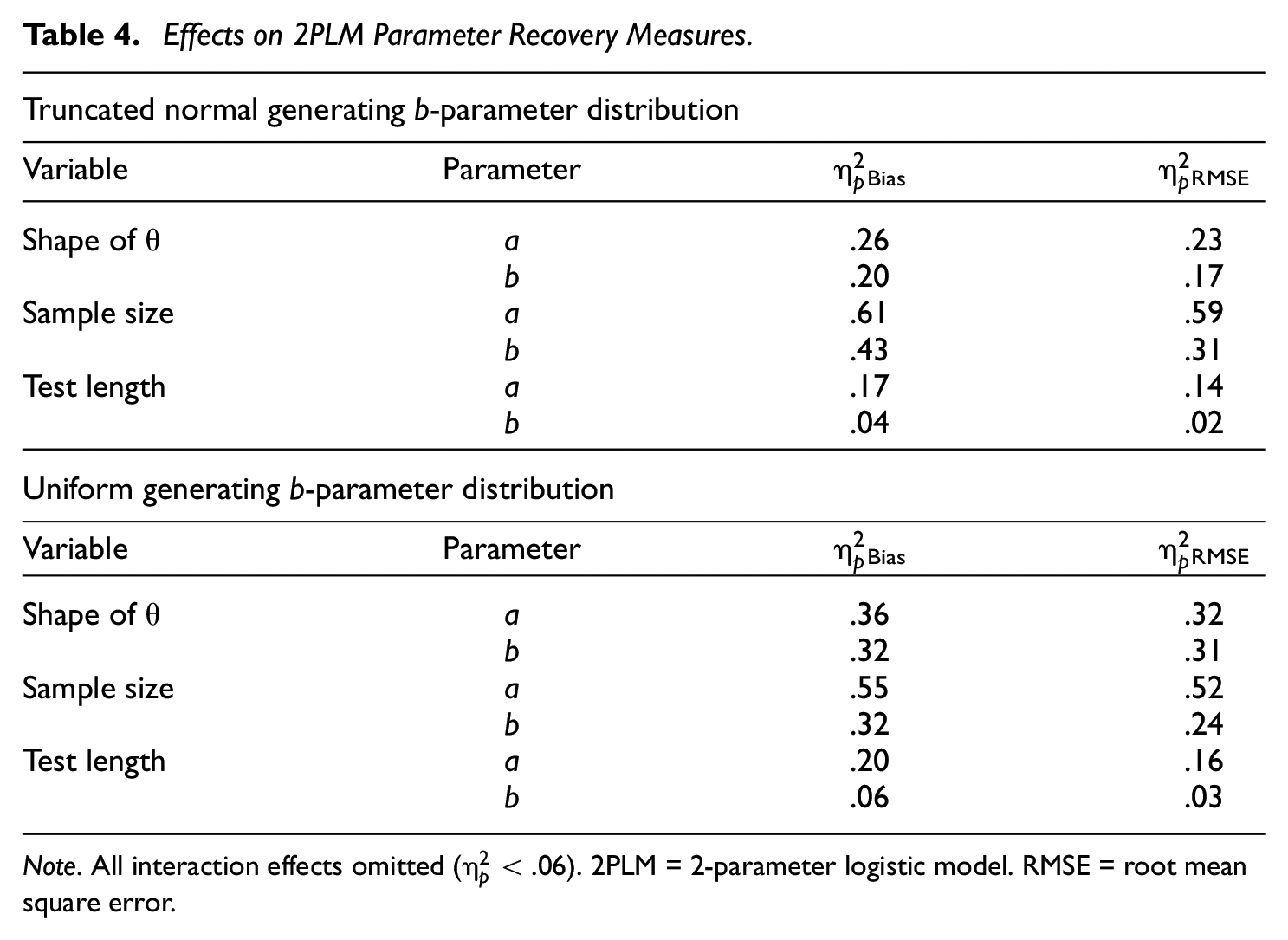
Note. All interaction effects omitted ( $η_{p}^{2}$ < .06). 2PLM = 2-parameter logistic model. RMSE = root mean square error.

Parameter Recovery for Converged Solutions

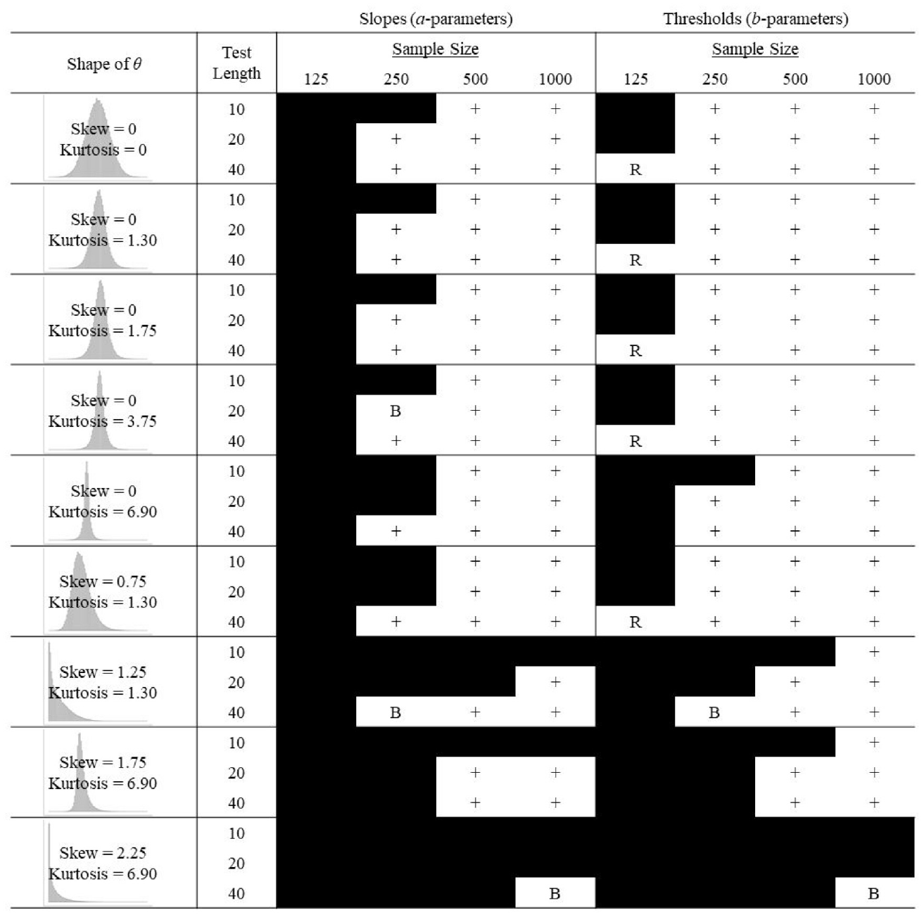
Based on the results of the ANOVAs, we focused our attention on sample size and the shape of θ when deciding which conditions led to acceptable parameter recovery. Tables with mean absolute bias and RMSE for each condition across the GRM, 2PLM_TN, and 2PLM_U are provided in the supplemental material. Figures 2 to 4 summarize Supplemental Tables S1 to S6. A plus sign (+) indicates that both mean absolute bias and RMSE, on average, were within the range of acceptable recovery (i.e., mean absolute bias and RMSE were both less than or equal to their respective cutoffs from Table 1). A “B” indicates that only mean absolute bias (but not RMSE), on average, was within the range of acceptable recovery. Similarly, an “R” indicates that only RMSE (but not mean absolute bias), on average, was within the range of acceptable recovery. A blacked out cell indicates that neither mean absolute bias nor RMSE, on average, fell within the range of acceptable recovery.

Figure 2.

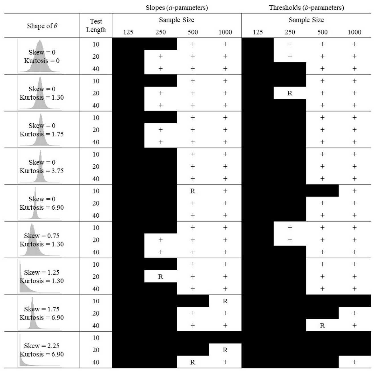
Summary of GRM Parameter Recovery for Converged Solutions.

Figure 3.

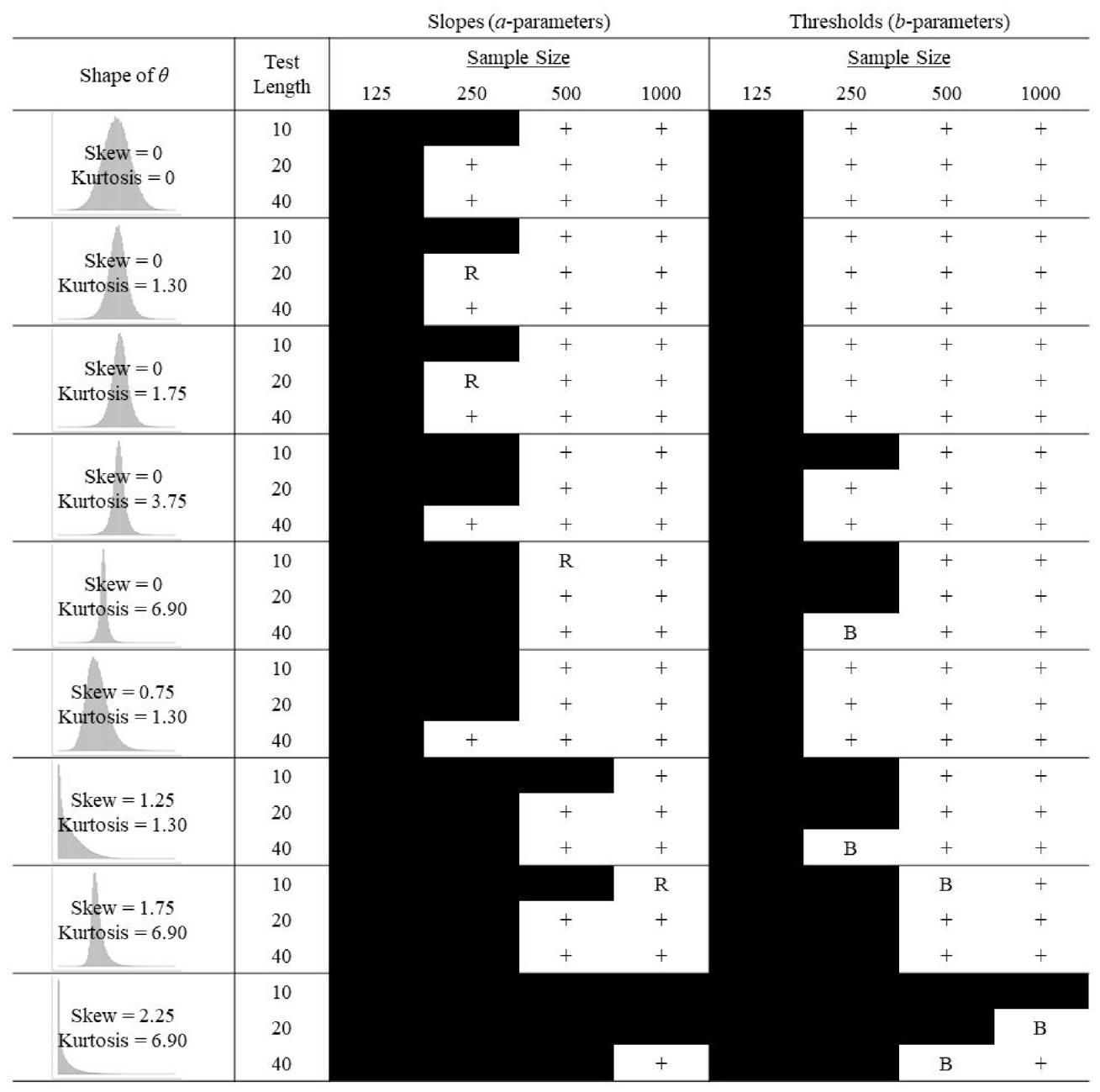
Summary of 2PLM_TN Parameter Recovery for Converged Solutions.

Figure 4.

Summary of 2PLM_U Parameter Recovery for Converged Solutions.

Beginning with slopes for the GRM (Figure 2), parameter recovery was unacceptable by both measures (mean absolute bias and RMSE), on average, for the control condition when sample size was 125. For N = 250, a test length of 10 items also led to unacceptable recovery by both measures. Longer test lengths for N = 250 (20 and 40), however, resulted in acceptable recovery by both measures. All test lengths with the larger sample sizes of N = 500 and N = 1,000 led to acceptable recovery by both measures. When introducing kurtosis, the pattern of results for the control condition held except for the two most severe levels of kurtosis. For a kurtosis of 3.75 and 6.90, average estimates for all test lengths with N = 250 became unacceptable by both measures. When introducing a skew of 0.75 to a kurtosis of 1.30, the pattern of results was the same when compared with no skew with a kurtosis of 1.30. There was a small difference when increasing the skew from 0.75 to 1.25 (N = 250 and test length = 40 became unacceptable by both measures, N = 250 and test length = 20 became unacceptable by mean absolute bias). When skew was increased from 0 to 1.75 (keeping kurtosis constant at 6.90), recovery became unacceptable by RMSE for N = 500 and test length = 10 and unacceptable by mean absolute bias for N = 1,000 and test length = 10. Increasing skew from 1.75 to 2.25 left only a single condition with acceptable recovery by both measures (N = 1,000 and test length = 40).

Compared with the recovery of slopes for the GRM, there was a greater impact of skew and kurtosis on estimates of thresholds (greater overall values of mean absolute bias and RMSE). For kurtosis specifically, recovery of slopes was worse by both measures for shorter test lengths and recovery of thresholds was worse by both measures for longer test lengths. Other than these differences, the pattern of results for recovery of thresholds compared with slopes was roughly the same.

Moving onto the 2PLM, we begin with the results that used a truncated normal distribution to generate b-parameters (2PLM_TN; Figure 3). The pattern of results for recovery of slopes was similar to the GRM. The sample size of 125, on average, consistently led to unacceptable recovery by both measures. However, compared with the GRM, the 2PLM_TN appeared to be slightly less robust to nonnormality and did not perform as well with smaller sample sizes (e.g., 250). The two milder kurtosis conditions (1.30 and 1.75) were identical. The minor difference from the control to these conditions was that N = 250 and test length = 20 became unacceptable by mean absolute bias. This condition also became unacceptable by RMSE when kurtosis was increased to 3.75. When further increased to a kurtosis of 6.90, a sample size of 250, on average, was no longer viable for any test length. There was not much of a change when introducing a skew of 0.75 to a kurtosis of 1.30 but when skew was increased from 0.75 to 1.25, two additional conditions resulted in unacceptable recovery by both measures (N = 250 and test length = 40; N = 500 and test length = 10). There was a minor change when introducing a more severe skew of 1.75 to the more severe kurtosis of 6.90. However, as with the GRM, combining the most severe skew (2.25) with the most severe kurtosis (6.90) left only a single condition with acceptable recovery by both measures (N = 1,000 and test length = 40).

Compared with the recovery of slopes under 2PLM_TN, slopes under the 2PLM_U (Figure 4) exhibited the same overall pattern of results aside from a few small differences. The 2PLM_TN appeared to be slightly more robust to skew, whereas the 2PLM_U was slightly more robust to kurtosis. Compared with slopes for both the 2PLM_TN and 2PLM_U, thresholds were more robust to nonnormality and better recovered in small sample sizes (opposite to the trend for the GRM). However, the pattern of results for thresholds was very similar to the pattern of results for slopes for each respective generating distribution. Although the pattern of results for recovery of slopes was very similar across all models (GRM, 2PLM_TN, and 2PLM_U), recovery of thresholds was better, on average, for the 2PLM_TN and 2PLM_U compared with the GRM.

Averaging across all conditions, mean absolute bias and RMSE were consistently higher for the 2PLM_U compared with the 2PLM_TN. This was expected because, controlling for the limits of the distributions, drawing b-parameters from a uniform distribution as opposed to a truncated normal distribution increases the frequency of extreme values. Consistent with Woods and Thissen (2006), bias increased when b-parameters reached or exceeded values of ± 2.

Discussion

The purpose of this study was to identify the type(s) and degree(s) of nonnormality that are most detrimental to estimation of the GRM and 2PLM. Previous simulation work has demonstrated that the misspecification of θ as normal, when it is nonnormal, results in biased parameter estimates when fitting unidimensional IRT models (Preston & Reise, 2013; Woods, 2006, 2007; Woods & Thissen, 2006). Corrections for nonnormality have been developed which solve the problem of θ misspecification but at a cost of computational intensity. This is especially problematic when the sample size is small-as is common in psychological research. With feasibility in question, we were interested in what kind and how much nonnormality could be tolerated for the more computationally convenient choice of assuming normality.

Overall, sample size and the shape of θ had the greatest impact on the ability of models to converge and the recovery of parameter estimates. Especially problematic were the smallest sample size of 125 and the most severe nonnormality with the largest degree of skew (2.25) and kurtosis (6.90). Neither resulted in acceptable recovery for any condition based on the Stone (1992) criteria. It is important to note that although parameters seemed to be recovered better with longer test lengths of 20 and 40, these test lengths also converged less often often (sometimes, much less) than the shorter test length of 10. The N = 125 and test length = 40 conditions for the GRM did not converge even once across the nine different shapes of θ.

In the best-case scenario, when the θ normality assumption was met, a sample size of 125 was not sufficient to achieve acceptable recovery. Sample sizes of 250, 500, and 1,000, however, appeared to be enough for acceptable estimation. When θ was nonnormal, a sample size of 125 was again not sufficient to achieve acceptable recovery for the GRM or 2PLM. For the GRM, a sample size of 250 was also not sufficient. With the exception of the two most severe nonnormality conditions, sample sizes of 500 and 1,000 were able to achieve acceptable recovery even if θ was nonnormal. For the 2PLM, a sample size of 250 was borderline when θ was kurtotic—acceptable recovery was achieved for some conditions. However, when θ was skewed, a sample size of 250 resulted in unacceptable recovery for the 2PLM. Aside from the most severe nonnormality condition, sample sizes of 500 and 1,000 led to acceptable 2PLM estimates when θ was nonnormal.

In summary, a sample size of 125 was too small regardless of whether the θ normality assumption was met or not. Given that sample size when estimating the GRM or 2PLM was at least 250, increasing sample size helped curb the effects of nonnormality on the recovery of parameter estimates. However, larger sample sizes did not protect against all nonnormality. If nonnormality is severe enough, then estimating the GRM or 2PLM with the normality assumption (often a program default) is no longer a tenable option. Generally, recovery gets worse as either skew or kurtosis increases, which is consistent with previous nonnormality work (e.g., Stone, 1992; Woods & Thissen, 2006). In addition to this, we found the tendency for skew to have a greater impact than kurtosis.

In this simulation study, we generated data based on a known and prespecified “true” latent trait distribution (θ). As “true”θ is unknown in practice, if indeed such a thing exists at all, the shape of the latent trait distribution is really a statistical and psychometric choice. In some cases, where one is approaching IRT as a statistical model fitting exercise, the data may fit better if the latent variable can take some shape other than a normal distribution. In other cases, when one is trying to make valid inferences regarding what scores mean, the shape of the latent variable may also be driven by theory. Ultimately, it is up to the researcher to decide whether normality is appropriate and, if not, what kinds of departures are consistent with theory. If theory suggests the shape of θ is nonnormal, the results of this study suggest that the unidimensional GRM and 2PLM are robust to violations of normality and permissible under specific circumstances. With a sample size of at least 500, the GRM is robust to six nonnormal θs (top three rows of Figure 1), given they were the actual generating distributions. The 2PLM is robust to four kurtotic θs (first row of Figure 1) if sample size is at least 250. With a sample size of at least 500, the 2PLM is also robust to three additional skewed and kurtotic θs (Rows 2 through 4 in Figure 1).

In terms of the differing generating b-parameter distributions for the 2PLM, our results suggest a recommendation for IRT simulations in general. Results were consistently different depending on the b-parameter generating distribution, so when presenting simulation results, this choice should be clearly stated. While this difference is perhaps not surprising, it underscores the importance of designing simulations to mirror what we are seeing in the real world to maximize their usefulness.

The results and recommendations presented in this article are intended to serve as a guide for when theory posits that a latent variable, trait, or construct may not follow a normal distribution. Although we were able to examine the robustness of the GRM and 2PLM to eight different combinations of skew and kurtosis (excluding the normal control), there are many avenues for improvement and expansion. As a starting point for this line of research, we limited our examination to unidimensional IRT models. As many psychological constructs and scales are multidimensional, it would be useful to examine whether the results of this study hold for the multidimensional extensions of the GRM and 2PLM. Despite the added complexity of multidimensional IRT (MIRT) models, the development of more efficient estimators (Cai, 2010a, 2010b), along with approaches for simulating multidimensional nonnormality that offer control over the degree of skew and kurtosis (Qu et al., 2020), vastly improves feasibility.

Another potential limitation was the choice of generating parameter distributions. For example, a-parameters were sampled based on work done by Hill (2004) who derived a distribution of slopes based on fitting the GRM to 15 psychological tests. While this distribution of slopes may be representative and perfectly reasonable to use for latent traits that are theoretically normally distributed, the implications of using this distribution of slopes when the underlying trait is theoretically nonnormal are unclear.

In addition, future work that delves deeper into issues of nonnormality and small sample size is warranted. When the latent trait distribution was nonnormal, this study found that the computationally convenient method of assuming normality was detrimental to estimation when sample size was small. Future studies could examine the feasibility of implementing the more computationally demanding nonnormality corrections or, ideally, other methods that would address both nonnormality and small sample size simultaneously. Finally, if it is viable to use nonnormality corrections for small samples, it would be interesting to see whether the shape of the latent trait distribution could be reasonably recovered. This would be in line with the work done by Woods and Thissen (2006) who illustrated the recovery and characterization of the latent trait distribution using both EH and RC-IRT methods. The results presented here can be used to guide future work on the effectiveness of these approaches as we have highlighted in detail under what conditions robustness to violations of the normality assumption are problematic.

Supplemental Material

sj-docx-1-epm-10.1177_00131644211063453 – Supplemental material for Examining the Robustness of the Graded Response and 2-Parameter Logistic Models to Violations of Construct Normality

Supplemental material, sj-docx-1-epm-10.1177_00131644211063453 for Examining the Robustness of the Graded Response and 2-Parameter Logistic Models to Violations of Construct Normality by Patrick D. Manapat and Michael C. Edwards in Educational and Psychological Measurement

Footnotes

Declaration of Conflicting Interests

The authors declared no potential conflicts of interest with respect to the research, authorship, and/or publication of this article.

Funding

The authors received no financial support for the research, authorship, and/or publication of this article.

ORCID iD

Patrick D. Manapat

Supplemental Material

Supplemental material for this article is available online.

Notes

References

Cai

(2010a). High-dimensional exploratory item factor analysis by a Metropolis-Hastings Robbins-Monro algorithm. Psychometrika, 75(1), 33–57. https://doi.org/10.1007/s11336-009-9136-x

Cai

(2010b). Metropolis-Hastings Robbins-Monro algorithm for confirmatory item factor analysis. Journal of Educational and Behavioral Statistics, 35(3), 307–335. https://doi.org/10.3102/1076998609353115

Cai

(2017). flexMIRT version 3.51: Flexible multilevel multidimensional item analysis and test scoring [Computer software]. Vector Psychometric Group.

Fleishman

A. I.

(1978). A method for simulating non-normal distributions. Psychometrika, 43(4), 521–532. https://doi.org/10.1007/BF02293811

Flora

D. B.

Curran

P. J.

(2004). An empirical evaluation of alternative methods of estimation for confirmatory factor analysis with ordinal data. Psychological Methods, 9(4), 466–491. https://doi.org/10.1037/1082-989X.9.4.466

Hill

C. D.

(2004). Precision of parameter estimates for the graded item response model [Unpublished master's thesis]. The University of North Carolina at Chapel Hill. https://catalog.lib.unc.edu/catalog/UNCb4556245

Houts

C. R.

Cai

(2016). flexMIRT user’s manual version 3.5: Flexible multilevel multidimensional item analysis and test scoring. Vector Psychometric Group.

Houts

C. R.

Edwards

M. C.

(2013). The performance of local dependence measures with psychological data. Applied Psychological Measurement, 37(7), 541–562. https://doi.org/10.1177/0146621613491456

Mislevy

R. J.

(1984). Estimating latent distributions. Psychometrika, 49(3), 359–381. https://doi.org/10.1007/BF02306026

10.

Pek

Wong

A. C. M.

(2018). How to address non-normality: A taxonomy of approaches, reviewed, and illustrated. Frontiers in Psychology, 9(NOV), 1–17. https://doi.org/10.3389/fpsyg.2018.02104

11.

Preston

K. S. J.

Reise

S. P.

(2013). Estimating the nominal response model under nonnormal conditions. Educational and Psychological Measurement, 74(3), 377–399. https://doi.org/10.1177/0013164413507063

12.

Liu

Zhang

(2020). A method of generating multivariate non-normal random numbers with desired multivariate skewness and kurtosis. Behavior Research Methods, 52(3), 939–946. https://doi.org/10.3758/s13428-019-01291-5

13.

Ramsay

J. O.

(2000). Differential equation models for statistical functions. Canadian Journal of Statistics, 28(2), 225–240. https://doi.org/10.2307/3315975

14.

R Core Team. (2020). R: A language and environment for statistical computing. R Foundation for Statistical Computing. https://www.r-project.org/

15.

Reise

S. P.

Rodriguez

Spritzer

K. L.

Hays

R. D.

(2018). Alternative approaches to addressing non-normal distributions in the application of IRT models to personality measures. Journal of Personality Assessment, 100(4), 363–374. https://doi.org/10.1080/00223891.2017.1381969

16.

Reise

S. P.

Waller

N. G.

(2009). Item response theory and clinical measurement. Annual Review of Clinical Psychology, 5, 27–48. https://doi.org/10.1146/annurev.clinpsy.032408.153553

17.

Samejima

(1969). Estimation of latent ability using a response pattern of graded scores (Psychometric Monograph No. 17). Psychometrika, 34(Suppl. 1), 1–97. https://doi.org/10.1007/BF02290599

18.

Shen

Kiger

T. B.

Davies

S. E.

Rasch

R. L.

Simon

K. M.

Ones

D. S.

(2011). Samples in applied psychology: Over a decade of research in review. Journal of Applied Psychology, 96(5), 1055–1064. https://doi.org/10.1037/a0023322

19.

Stone

C. A.

(1992). Recovery of marginal maximum likelihood estimates in the two-parameter logistic response model: An evaluation of MULTILOG. Applied Psychological Measurement, 16(1), 1–16. https://doi.org/10.1177/014662169201600101

20.

Woods

C. M.

(2006). Ramsay-curve item response theory (RC-IRT) to detect and correct for nonnormal latent variables. Psychological Methods, 11(3), 253–270. https://doi.org/10.1037/1082-989X.11.3.253

21.

Woods

C. M.

(2007). Empirical histograms in item response theory with ordinal data. Educational and Psychological Measurement, 67(1), 73–87. https://doi.org/10.1177/0013164406288163

22.

Woods

C. M.

Thissen

(2006). Item response theory with estimation of the latent population distribution using spline-based densities. Psychometrika, 71(2), 281–301. https://doi.org/10.1007/S11336-004-1175-8

Supplementary Material

Please find the following supplemental material available below.

For Open Access articles published under a Creative Commons License, all supplemental material carries the same license as the article it is associated with.

For non-Open Access articles published, all supplemental material carries a non-exclusive license, and permission requests for re-use of supplemental material or any part of supplemental material shall be sent directly to the copyright owner as specified in the copyright notice associated with the article.

0.00 MB

0.08 MB