
Abstract
Situational judgment tests have gained popularity in educational and psychological measurement and are widely used in personnel assessment. A situational judgment item presents a hypothetical scenario and a list of actions, and the individuals are asked to select their most likely action for that scenario. Because actions have no explicit order, the item generates nominal responses consisting of the actions selected by the individuals. This article shows how to factor-analyze the nominal responses originated from such a test, including the estimation of the number of latent factors and a factor invariance analysis in a multiple group design. The method consists of applying the MNCM, a multidimensional extension of the nominal categories model by Bock. The article includes the results of two studies: (1) a simulation study about Type-I error rate, statistical power, and recovery of the parameters in a multigroup factorial invariance design and (2) a real data example using responses to a situational judgment test measuring gender stereotypes to illustrate the approach. Results suggest the use of the Akaike information criterion, Bayesian information criterion, and corrected Bayesian information criterion indices to guide the selection of the number of factors with nominal responses. All the analyses are conducted using the computer program Mplus. The code is included as Supplemental Material (available online) for the readers so that they can adapt it to their own purposes.
Keywords
Items from a situational judgment test (SJT) present a situation followed by a set of hypothetical response categories that the individual might choose in that situation. The task of the test takers consists of selecting the response option that best represents their way of behaving in that particular scenario (Lievens et al., 2008; McDaniel & Nguyen, 2001). SJTs have been widely used in industrial and organizational psychology (Ployhart & Ward, 2013), but they have gained popularity over recent years and have been extended to education and other contexts for the assessment of constructs, such as interpersonal skills, leadership development, and so on. Unlike other test items formats, in a SJT the response categories consist of a list of behaviors that lacks an explicit order, thus the items are scored as nominal categories. However, the basic questions of psychological measurement are still relevant for such a test. This article shows how to respond to the question of what is the factorial structure of a SJT scored in nominal categories.
The traditional approach to factor analysis is not immediately applicable to the SJTs because the factor analysis model assumes that scores have at least an ordinal measurement level (Floyd & Widaman, 1995). One solution to this problem is to assign arbitrary scores to the response categories of a SJT and assume that these scores are suitable for classical statistical analyses (Sharma et al., 2013). However, apart from being arbitrary, the weights are implicitly based on the premise that the data are one-dimensional and afterward, they are used to test dimensionality, which is a rather circular argument. More recently, Zu and Kyllonen (2018) proposed to use Bock’s model to score SJT to avoid the assignment of arbitrary scores. However, Bock’s model assumes a one-dimensional latent structure and does not solve the problem of estimating the number of latent factors. This article builds on Zu and Kyllonen (2018) and uses a multidimensional extension of Bock’s model to estimate the number of factors and the factorial structure.
Multidimensional extensions of Bock’s model were suggested by Takane and de Leeuw (1987), Thissen et al. (2010), Revuelta (2014) and Thissen and Cai (2016). The multidimensional nominal categories model (MNCM) explains the distribution of the manifest variables by appealing to a vector of latent factors, and the relation between response categories and latent factors is estimated from the matrix of individual by item responses. The MNCM has been applied by Revuelta et al. (2020) to perform exploratory and confirmatory factor analyses from item responses that do not have an explicit order.
This article presents procedures based on the MNCM for the analysis of the factorial structure in SJTs. It also extends the MNCM to the multigroup analysis of factorial invariance for nominal data provided by a SJT. The article is organized in five sections. First, a Scale of Gender Stereotypes (SGS) is presented to illustrate a SJT and the type of data that motivates the subsequent theoretical developments. The SGS is a SJT in which each item presents a scenario for a group of characters and contains response categories representing different ways of behaving, thus generating nominal response data. Two different forms of the SGS were created, differing in the wording with which the group of characters is presented, and both forms have been applied to different samples of individuals, thus motivating a multigroup analysis. The second section contains the theoretical aspects, including the mathematical formulation of the MNCM and the different levels at which factorial invariance can be investigated. Third, a simulation study is presented to gather information about the capabilities of the methods to estimate the number of latent factors, test hypotheses about factor invariance, and the recovery of the parameters in realistic conditions. The fourth section of the article includes a real data analysis that consists of an empirical study estimating the number of latent factors and investigating factorial invariance for the SGS. Finally, a general discussion summarizes the results of the simulation and the empirical studies and concludes the article.
All the analyses were performed using the computer program Mplus (Muthén & Muthén, 1998-2017). The estimation algorithms and fit statistics are purposely restricted to those included in Mplus to facilitate the dissemination of these methods, as Mplus is one of the most accessible and widely used software for fitting latent variable models. The Mplus code is available in the Supplemental Material (available online) so that the readers may adapt it to their own data.
A Situational Judgment Test of Gender Stereotypes
The SGS consists of 10 items presenting brief scenarios. Each scenario includes a group of characters in a certain situation, and the item contains three response categories that represent behaviors that such characters may follow in that situation. The test takers must choose which behavior is more plausible for the group in the situation presented. The content of the scenarios has been designed based on the gender stereotypes of the traits and roles dimensions collected in López-Sáez et al. (2008). Five items are extracted from the stereotypes related to the personality traits socially assigned to men and women (Items X1 to X5), and the other five items with the stereotypical social roles of both genders (Items X6 to X10). The response categories are designed to represent a supposedly male, female, or neutral stereotypical way of behaving in the situation posed by the item.
Two forms of the test were created differing in the terms used to present the characters of the story. For both forms, the group of characters is assumed to be gender mixed. The SGS is written in Spanish language, and the two forms differ in the linguistic markers used to denote the characters of the story. For example, imagine that you want to write about your group of friends. In Spanish, the morpheme “-o” is reserved for the masculine grammatical gender as well as for the generic he (i.e., the masculine generics, MG), so that the Spanish word amigos (friends) denotes both a group of friends composed only of men, or a group composed of men and women. The word amigas denotes a group of friends composed only of women, and the alternative generics (AG) amigos/as explicitly emphasizes that the group is gender-mixed.
In the first form of the SGS, the group is mentioned using the MG (e.g., amigos); and in the second form, using the AG (e.g., amigos/as). The purpose of developing two forms of the test is to investigate whether or not the wording of the generic (which is currently a strong international debate) affects the gender stereotypes that they elicit in the individuals responding to the test. An English translation of the SGS is presented in the Supplemental Material (available online) of this article, as well as the Spanish wording of the MG and AG forms.
Responses to the SGS consists of nominal categories. However, as the task of the respondent is to select the most plausible category, we can assume that there is an underlying order of preference between categories that can be estimated from the data. The purpose of the data analysis of the SGS is twofold: First, we want to know how many latent factors are measured by the test, and second, we want to investigate whether the factorial structure of the SGS differs from the MG and AG forms of the questionnaire. According to previous findings on gender stereotypes, we formulated two hypotheses as follows:
More specifically, our interest is to know whether the stereotypically male-categories will be more frequently selected when using MG as compared to AG. Most of the previous studies in the literature about gender stereotypes have addressed these questions by using simple frequency comparisons (Hamilton, 1988; Kaufmann & Bohner, 2014; Merritt & Kok, 1995; Nissen, 2013). However, the application of the MNCM makes it possible to explore these hypotheses in a novel way, based on latent variable models for nominal responses.
Theoretical Background
The MNCM is an extension of the (one-dimensional) nominal categories model by Bock (1972) and Bock and Gibbons (2010) to the multidimensional latent space. The MNCM has been successfully applied to conduct exploratory and confirmatory factor analyses from nominal responses (Revuelta, 2014; Revuelta et al., 2020). In this article, the MNCM is extended to the multi-group research design and applied to a real data sample from the SGS.
Multinomial Probit and Logit Models
The MNCM assumes that the individuals who respond to a nominal item can rank order the categories according to their preferences. In this nominal response format, which is called first-choice data, the selected category is the most preferred one. More specifically, suppose that an item is scored in

Utilities depend on a vector of

where
Category
For a fixed value of
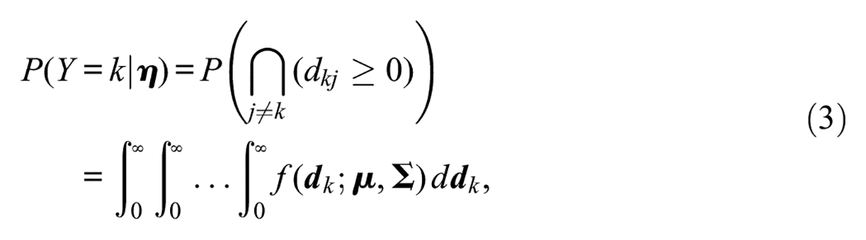
where
Equation (3) is difficult to compute because it involves a
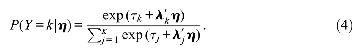
In practice, response probabilities are computed using Equation (4) for mathematical simplicity. McFadden (1974) showed that the approximation (4) to (3) is exact when the errors,
Model parameters are unidentifiable because the probabilities depend on differences between utilities, and if a constant value is added to all the utilities, the differences remain unaltered. To remove this arbitrariness, one of the categories (say category
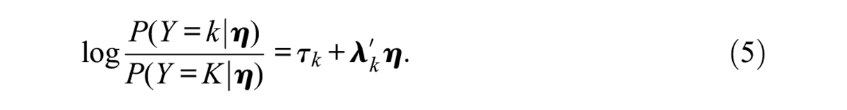
The intercept parameter,
Removing Latent Indeterminacy in Exploratory Nominal Factor Analysis
The distribution of the latent factors is assumed to be

where
Let
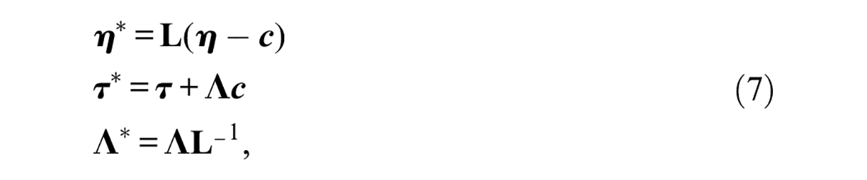
where
The practical consequence of this indeterminacy is that
These constraints in
Note that these constraints still leave the problem of reflection indeterminacy unresolved. That is, the model remains the same if the factor scores and the slopes are multiplied by −1. However, this indeterminacy can be easily resolved after estimation by inverting the sign of the slopes if desired.
Multigroup Factor Analysis for Nominal Data and Levels of Invariance
The multigroup MNCM assumes that the population of individuals is divided into
A multigroup analysis is useful to compare factorial structures and test hypotheses of parameter equality across groups (Raju et al., 2002). However, these tests need to be performed in a specific order to obtain meaningful results. For example, it is obvious that factor means cannot be compared across groups if the meaning of the factors varies. For these reasons, tests of equivalence are arranged in a sequence of nested models with increasingly strong equivalence levels (Vandenberg & Lance, 2000) as follows:
No invariance (NI). The factorial structure differs between groups, and all parameters are different. This is the baseline model, and it is useful to test hypotheses of invariance by comparing its fit with the one of a more constrained model.
Configural invariance (CI). The same factor structure holds across groups. The matrices
Weak invariance (WI). The factor loadings are equal across groups,
Strong invariance (SI). Factor loadings and intercepts (
A multigroup MNCM with external covariates is a type of model known as MIMIC (multiple indicator, multiple cause), and it regresses factor scores on a vector of manifest exogenous variables,

where
No invariance. The regression intercepts and slopes vary from one group to another.
Invariance of slopes. The regression slopes,
Invariance of slopes and intercepts. Both the regression intercepts and slopes are equal across groups. This level of invariance requires SI; otherwise it would be indeterminate if the differences in response frequencies across groups were due to the item intercepts or to the regression intercepts.
Inferential Aspects
In this article, the inferential algorithms will be restricted to those included in the Mplus (Version 8) computer program so that the readers can use them as a reference for their own potential applications. Bayesian estimation algorithms have also been proposed in the psychometric literature to overcome some of the limitations of the classic methods (Revuelta & Ximénez, 2017) but they will be not used in this article to keep the methods within the capabilities of Mplus.
Parameter Estimation and Likelihood Ratios
The MNCM is estimated from the matrix of responses of
The output provided by Mplus when fitting latent variable models for nominal data includes the maximum value of the log-likelihood, the number of free parameters, and the AIC, BIC, and BICc statistics (Vrieze, 2012). AIC and BIC are the Akaike information criterion and the Bayesian information criterion, respectively, and BICc is corrected BIC, that is, the BIC statistic adjusted by sample size proposed by Sclove (1987). The AIC, BIC, and BICc have been compared in the context of factor variable models by Tein et al. (2013), Chen et al. (2017), and Dziak et al. (2020).
The likelihood-ratio chi-square is computed as
The test of relative fit assumes that the mathematical form of the model is correct and uses the likelihood-ratio chi-square to compare models with different number of latent factors in exploratory analyses, or models with different levels of invariance in a multigroup analysis (Bentler, 1990).
Estimating the Number of Latent Factors
In an exploratory analysis, the number of latent factors could be estimated by comparing the fit of the model with
Multigroup Comparisons
The likelihood-ratio tests can also be applied in a multigroup analysis to compare models at different levels of factorial invariance. In our experience, this method is reliable in the investigation of invariance. However, the likelihood-ratio chi-square requires to estimate the model twice, with and without the parameter constraint to be tested. In many cases, a simpler approach based on a single estimation is more practical.
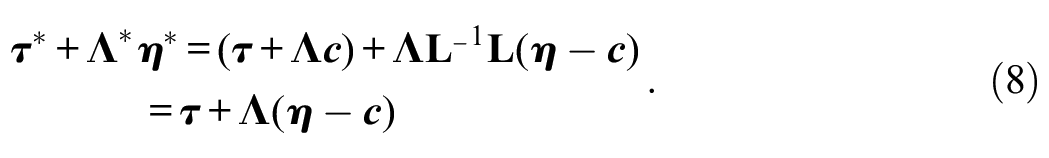
Contrast tests allow for great flexibility in the comparison of parameters; for example, to test the invariance item-by-item. Parameters can be compared within an item, from one item to another, and across groups. The null hypothesis for a contrast test is that a linear combination of item parameters is zero. Two contrast tests that will be applied below in this article are
The test of
Contrast tests can be easily implemented in Mplus using the MODEL CONSTRAINT command. The output of Mplus includes the test statistic, the standard error, and the p value for such a hypothesis. The test statistic provided by Mplus is the standardized estimated linear combination:
Simulation Study
A simulation study was designed to investigate the performance of the goodness-of-fit statistics in estimating the number of latent factors and detecting different degrees of model invariance between groups. As a secondary aim, we investigated the recovery of the parameters.
Method
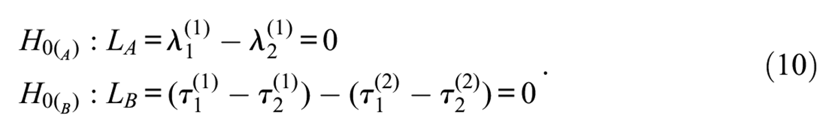
The simulation scenarios consisted of two groups with different levels of invariance. The number of items was 10, with three categories per item to recreate a realistic situation. The simulating model was one-dimensional. There are no external covariates (i.e., the MIMIC model) in the simulation study. The true values of
The true parameter values appear in Table 1. The symbols
True Parameter Values for the Simulation Study.
Note.
The simulated conditions were
Total sample size,
The effect size for parameter
Effect size for parameters
The total number of simulated conditions was

The values of
Analytic Strategy
The following models were estimated for each sample:
Configural invariance with one factor: This model assumes that all parameters
Configural invariance with two factors: This model was fitted to evaluate the Type I error rate when comparing fit against a model with unnecessary latent factors and to investigate whether invariance can be confounded with multidimensionality.
Model of weak invariance: The loadings are held constant across groups but the intercepts are allowed to vary. It is equivalent to the generating model in the conditions with
Model of strong invariance: It assumes equal loadings and intercepts across groups. It is equivalent to the generating model when
The analyzed statistics were those provided by Mplus:
Likelihood-ratio chi-square statistic: Model 1 was compared against Model 2, Model 3 against Model 1, and Model 4 against Model 1. The interpretation of a significant chi-square depends on the models being compared. Models 1 and 2 are correct for all the conditions because the simulating model falls within their parameter space. Models 3 and 4 are incorrect in general as they are more constrained than the simulating model. In the comparison 1–2, a significant chi-square was interpreted as a Type I error that consists of rejecting the true common-factor model in favor of a model with an spurious factor. In the comparisons 3–1 and 4–1, a significant chi-square is interpreted as an indication of statistical power. Note that in comparison 1–2, both models were always correct and the comparison gave an estimate of the Type I error rate when comparing a one-dimensional model against a two-dimensional model with a spurious latent factor. In comparisons 3–1 and 4–1, the Models 3 and 4 were generally wrong and were tested against Model 1, which was always correct; thus, these comparisons inform about statistical power. Type I error rate and statistical power were estimated by the empirical proportion of rejection (EPR), which is the proportion of samples in which the p value associated with the chi-square statistic is smaller than or equal to the nominal level (
Information measures: AIC, BIC, and BICc. For each condition, the model that minimized any given information measure was the model selected by that measure. The empirical proportion of selection (EPS) was the proportion of samples in which each of the four models minimized the AIC. The EPS associated to BIC and BICc were also computed.
Contrast tests were computed in relation to Model 1 to investigate the Type I error rate and power curves associated with these tests. Table 2 summarizes the contrast tests. The column labeled status of
Contrast Tests for the Simulation Study.
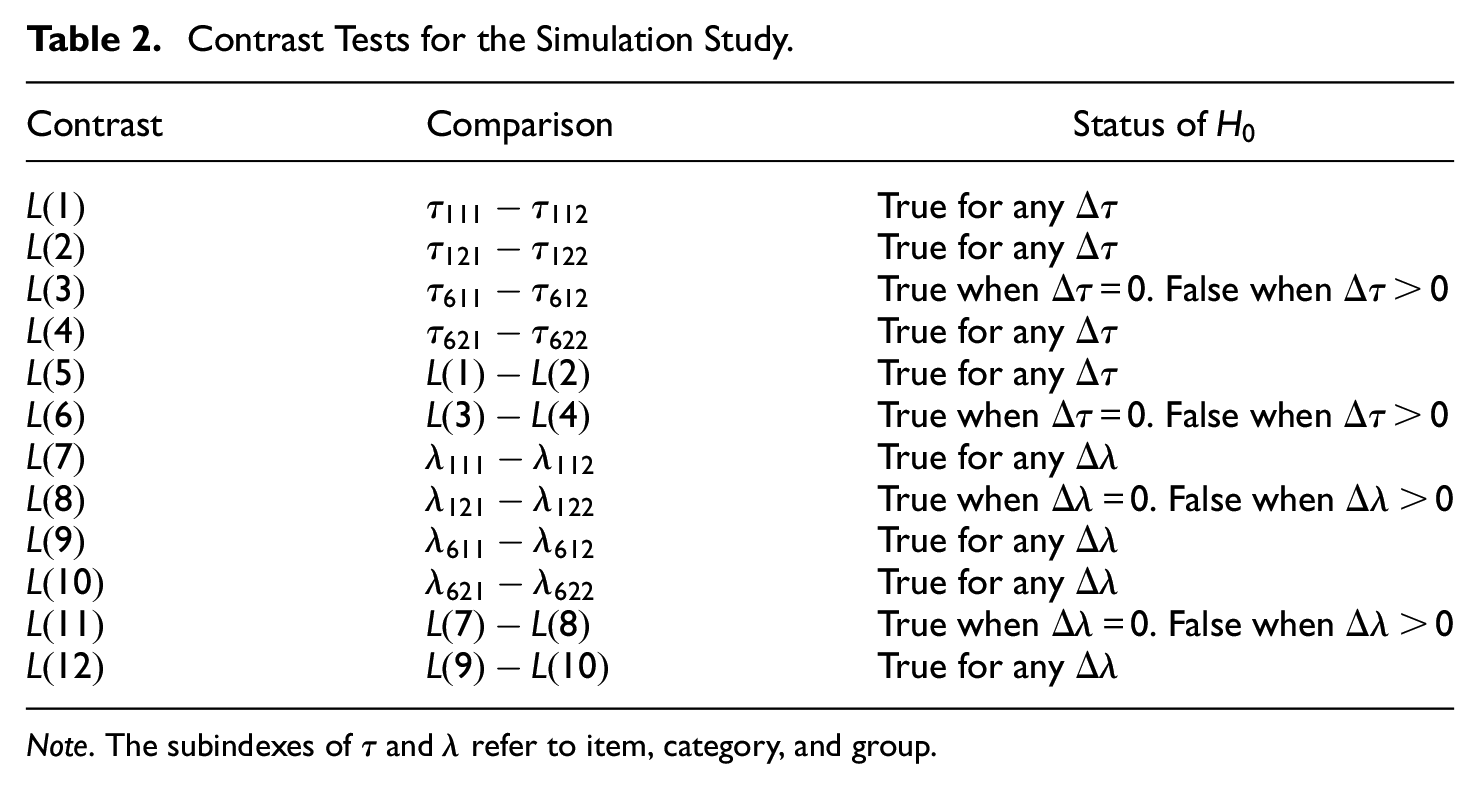
Note. The subindexes of
Results of the Simulation Study
Results for Chi-Square
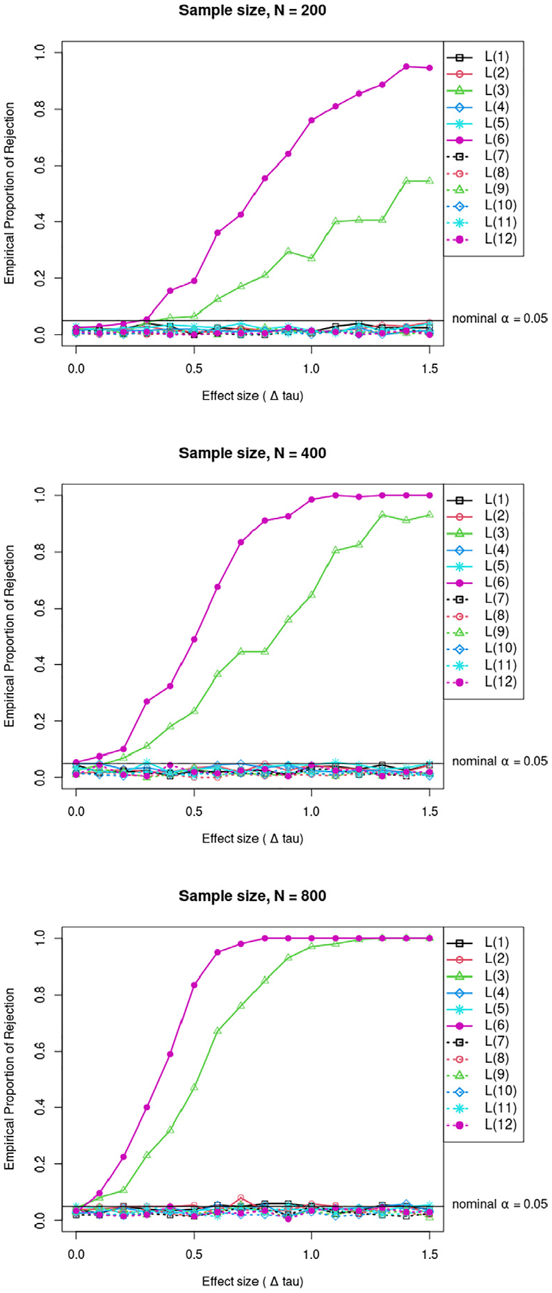
Results for the likelihood-ratio chi-square are summarized by the graphical representation of the EPR as a function of effect size (Figure 1), which is an estimate of the power curve. The upper panel represents the conditions with
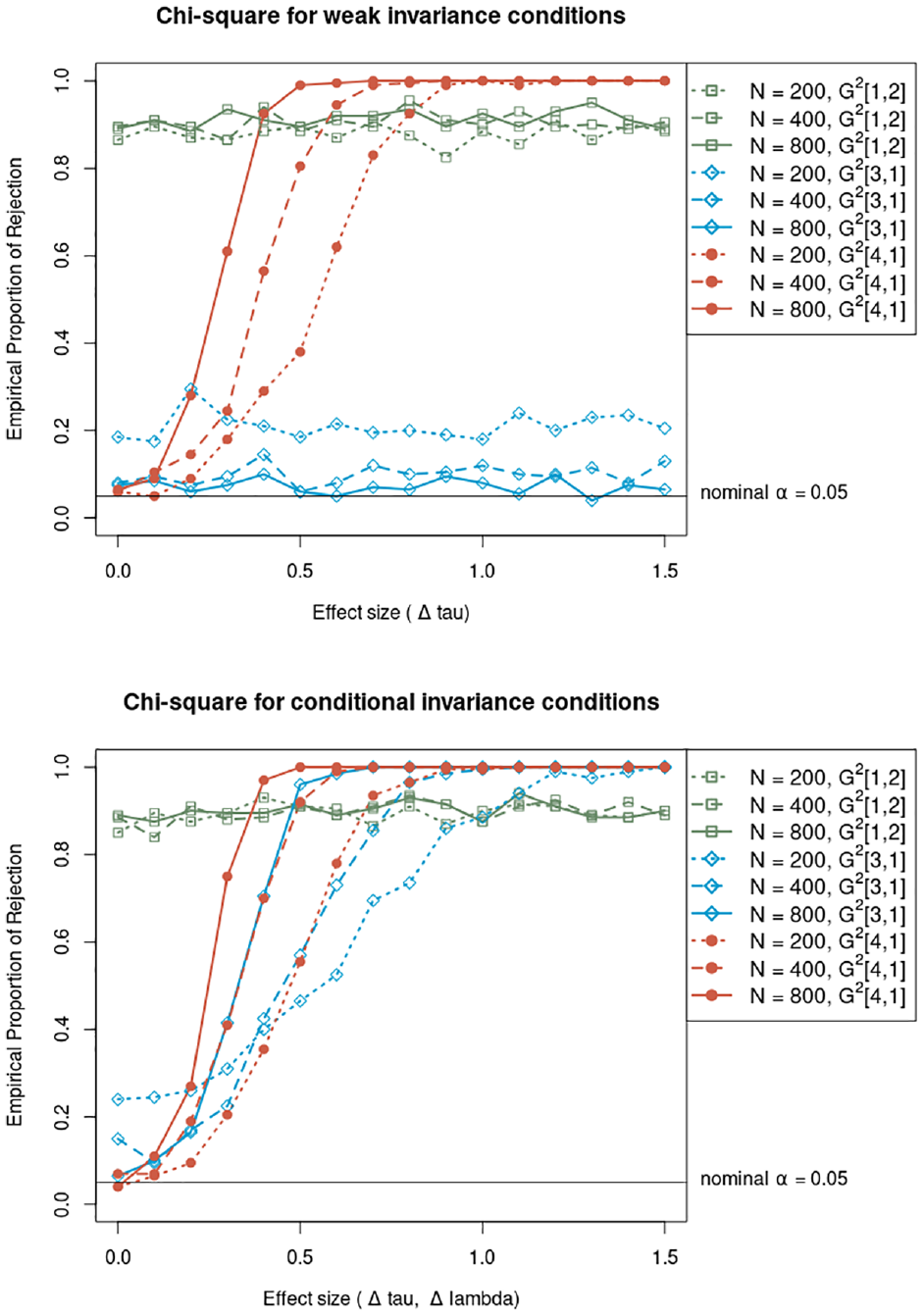
Empirical proportion of rejection for chi-square likelihood-ratio statistic as a function of effect size.
The lines with rhombus markers represent the EPR for the comparison between Models 3 and 1. In the upper panel, these lines are Type I error rate when comparing the true weak invariance model with a model that unnecessarily allows group differences both in the intercepts and in the slopes (i.e., the configural model). The results showed that chi-square was too liberal with the small sample size, with an EPR about 0.2 and approached the nominal level as the sample size increased. Thus, in real applications with small samples, there is a danger of erring in the direction of rejecting a true model of weak invariance in favor of a model with unnecessary free slopes. In contrast, the blue lines in the lower panel are an estimate of statistical power, as this time, slopes varied across groups and therefore Model 3 was false. The EPR increased sharply in relation to the effect size, approaching 1 for values of
The lines with spherical markers represent the comparison between Model 4 (which was true only when
All in all, the chi-square was very sensitive to detect model violations. When it comes to test model dimensionality, the chi-square lacks its utility because of its extremely liberal tendency. However, the chi-square proved to be useful to detect differences about 0.5 points or more between the model parameters of the two groups.
Results for AIC, BIC, and BICc
The EPS results for the conditions with
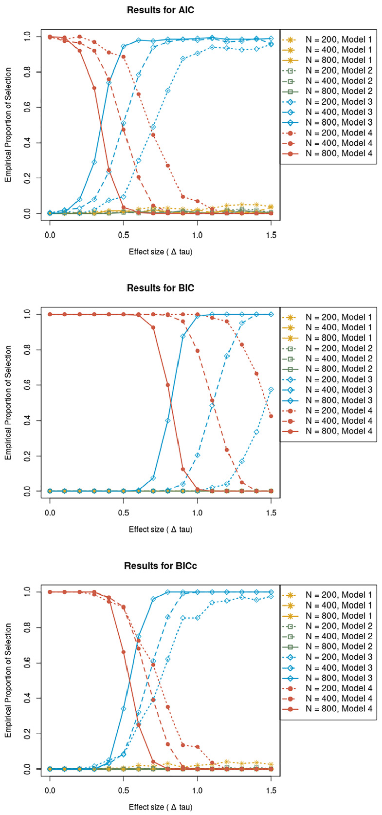
Empirical proportion of selection for the AIC, BIC and BICc as a function of effect size (
The results for
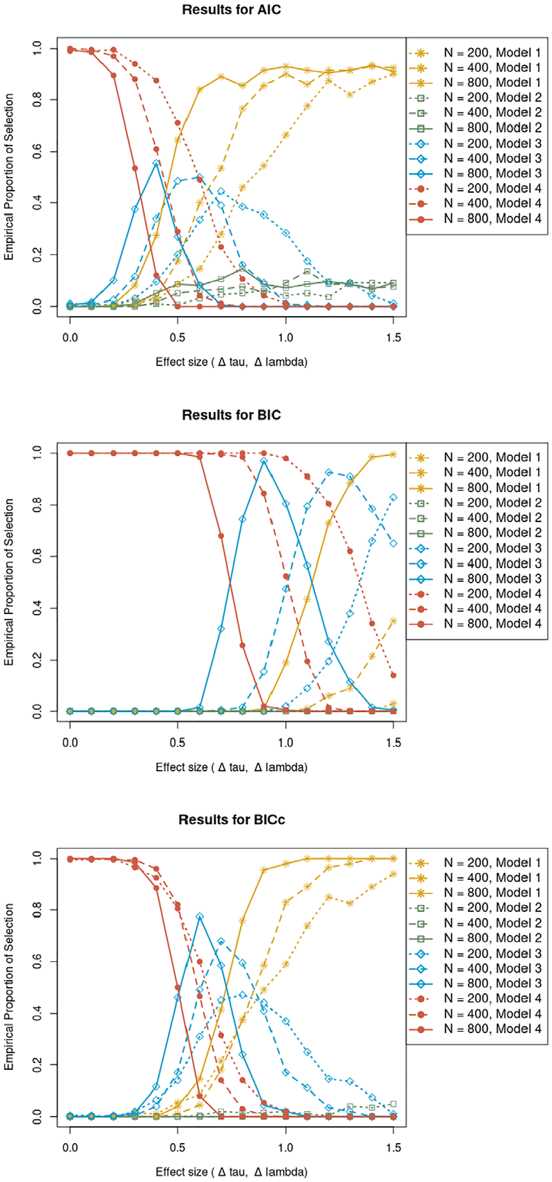
Empirical proportion of selection for the AIC, BIC, and BICc as a function of effect size (
Results for Contrast Tests
Contrast tests for
Contrast tests were computed to investigate the Type-I error rate and statistical power for Model 1. The
Figure 4 contains the EPR for all the contrast tests as a function of effect size. The figure shows that both
Empirical proportion of rejection for
Contrast tests for
In the conditions with
Figure 5 shows that the contrast tests for the slopes,
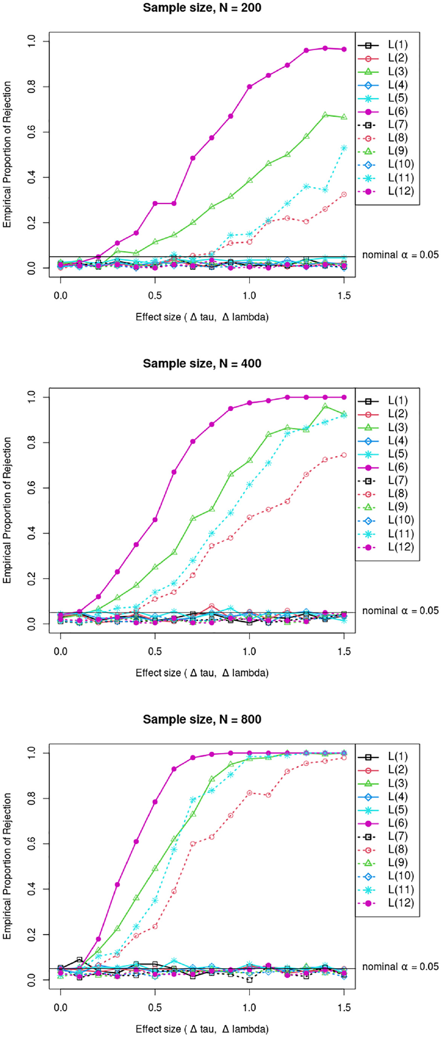
Empirical proportion of rejection for
Parameter Recovery
The simulation study also provided information about the recovery of true parameter values in realistic conditions regarding sample size and number of items. Recovery was evaluated by the mean bias and the root mean squared error (RMSE) between the true and estimated parameters for Model 1.
The means and standard deviations of the recovery statistics appear in Table 3. In order to keep the presentation to a minimum, the results were averaged over parameter types. In this sense, recovery was better for intercepts than for slopes. Moreover, the simulation indicated that at least 400 individuals seem necessary to obtain interpretable item parameters because of the poor recovery with smaller samples.
Recovery of the Parameters for the Configural Invariance Model.
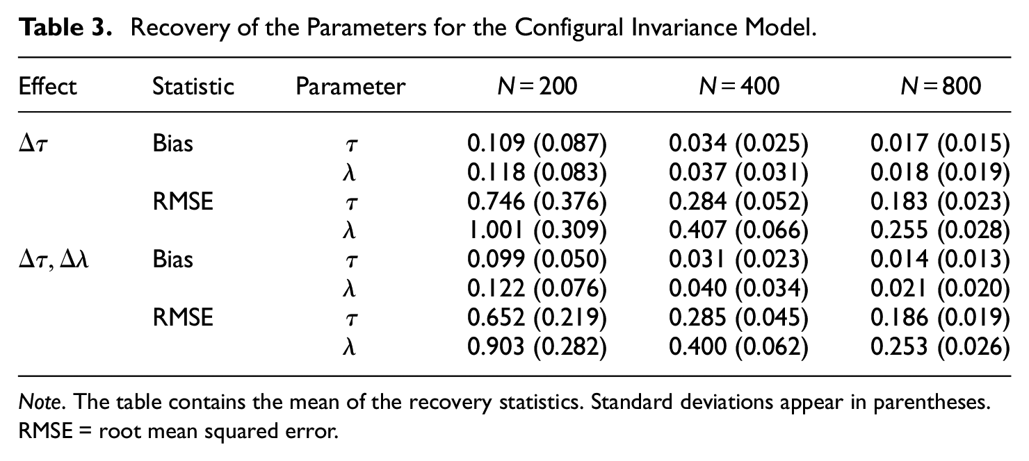
Note. The table contains the mean of the recovery statistics. Standard deviations appear in parentheses. RMSE = root mean squared error.
Conclusions of the Simulation Study
In summary, the goodness-of-fit statistics did a good job of detecting different levels of invariance. While the chi-square statistic was sensitive to violations of the assumption of invariance, the information statistics (AIC, BIC, and BICc) successfully identified the correct model, with a slight tendency for the AIC to select a too complex model. In addition, the contrast tests rendered reliable results about the item parameters that differ between groups and kept the Type I error rate at the nominal level when no such differences exist.
However, our results showed that the estimation of the number of factors cannot be based on chi-square. This statistic showed an extremely liberal tendency and selected an overfactored model in about 90% of the samples. Fortunately, the information statistics did not share this drawback and penalized the two-factor model in comparison to the models with one factor. All in all, chi-square is useful for testing model invariance, but when it comes to evaluating dimensionality, the decision should be based on information statistics.
Empirical Study
An empirical study was conducted to test the hypotheses presented in the section “A Situational Judgment Test of Gender Stereotypes” with a sample of real data and to put the recommendations extracted from the simulation study into practice.
Method
Two samples of 200 individuals were recruited, making a total of 400 participants, conforming a representative sample of young Spanish men and women. Each sample contains 100 men and 100 women who responded to one of the SGS forms (MG or AG), which were already explained in the section “A Situational Judgment Test of Gender Stereotypes.” The ages of the participants ranged from 17 to 30 years. The test was administered online through the Qualtrics platform. The presentation order of both the items and the categories was randomized. The sample contains no missing data because the online platform does not allow omitting responses. The recruitment of the participants was done through social networks such as Twitter and Instagram, as they are the most accessible media for our population of interest. The recruitment method allowed obtaining data from a less restricted sample, as participants could respond from different locations within Spain, so the results could be more generalizable. However, recruitment was limited to the Spanish participants. Each participant was randomly assigned to one of the two conditions (MG or AG), controlling that gender was balanced between both forms of the test. The conditions in the multigroup analysis (MG and AG) refer to test form, not to men and women. The purpose of collecting these data was to test the hypotheses previously presented in an empirical scenario.
Analytic Strategy
Five data analyses were conducted on the SGS data:
Preliminary descriptive analyses were used to obtain initial information about the data before running the inferential methods.
An exploratory nominal factor analysis (Revuelta et al., 2020) was conducted to identify the number of factors and to gather evidence about the theoretical assumption that the SGS is a one-dimensional instrument.
Measurement invariance between the two generic forms of the SGS (MG and AG) was tested to identify the level of invariance between the forms (Vandenberg & Lance, 2000). Supposedly, the use of one generic or another should not modify the construct measured by the test, and the data may thus support at least the level of weak invariance. The purpose of the analysis is to evaluate this hypothesis.
The third analysis consisted of delving further information by applying contrast tests to compare both forms of the SGS item-by-item. In other words, intercept and factor loadings for each item were compared between the two forms.
Last, factor scores were regressed on gender and age using the MIMIC model (Jöreskog & Goldberger, 1975).
Results of the Empirical Study
Descriptive Analysis
As can be seen in the bar-plot of Figure 6, at a descriptive level, there were little differences between the observed response frequency of the categories in the two groups. Specifically, the female-category had a higher frequency in the AG condition than in the MG condition for Item X7, whereas the reverse pattern occurred in Item X8, where the male-category had a higher frequency when using MG. The differences between conditions were small in the rest of the items.
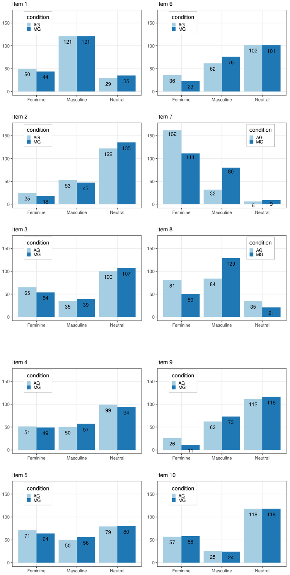
Response frequencies for the item categories in both groups.
Regarding the covariable age, the mean was 22.0, the standard deviation was 3.27, and the quartiles were
Exploratory Nominal Factor Analysis to Identify the Number of Factors
Exploratory nominal factor analysis models with one, two, and three factors were fitted to the SGS data. Model fit was compared by the likelihood-ratio chi-square, and the AIC, BIC, and BICc indices. The results appear in Table 4. In this regard, significant likelihood-ratio chi-square statistics were found between the one-factor and two-factors models, but not between the two- and three-factors models. However, the simulation study revealed that chi-square is too liberal, and information statistics are more reliable to estimate dimensionality. The model with two factors minimized the AIC, but the difference in AIC between the one-factor and the two-factor models was smaller than 2, which is the value suggested by Burnham and Anderson (2004) as an indication of substantial difference between AIC values. The BIC and BICc also supported the one-factor model. All in all, there was some evidence that there could be two factors underlying the item responses. However, this evidence was not strong, and we retained the one-factor model for further interpretation of the results. A larger sample could provide further information about this issue.
Goodness-of-fit Indices for the One-, Two-, and Three-Factors Models.
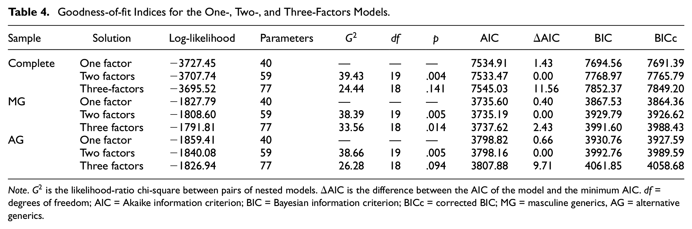
Note.
Measurement Invariance
The three levels of invariance (CI, WI, and SI) were compared for the one-factor model. The goodness-of-fit statistics appear in Table 5 and indicate that the chi-square statistic was not significant for the comparison between the CI and WI levels, but it was significant when comparing the WI and SI levels. In addition, the AIC favored the WI model, whereas the BIC and BICc indexes suggested the SI model.
Goodness-of-fit Indices for the Configural, Weak, and Strong Invariance Models.
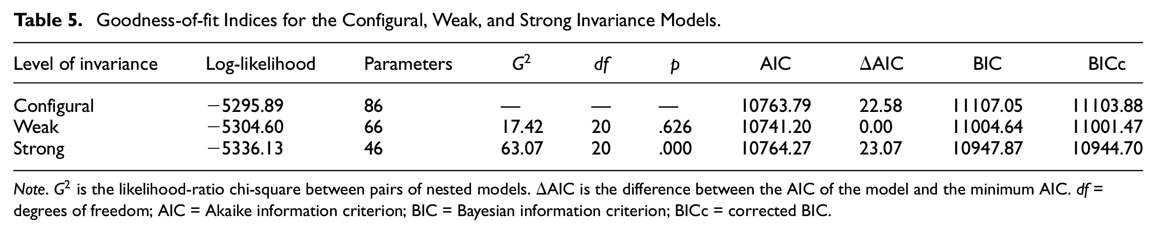
Note.
Item parameters and response functions were analyzed to investigate the differences between generic forms in more detail. Figure 7 contains the path diagram and item parameters for the WI model. We have slightly modified the conventions for a path diagram to accommodate the peculiarities of the nominal variables. In this regard, the path that goes from the factor to each item splits into two arrows, one for each of the categories that have estimated parameters. The arrow of each category is labeled with the slope and the intercept (in brackets). The parameters for the third category (the neutral option) are structural zeros and are not represented in the path diagram.
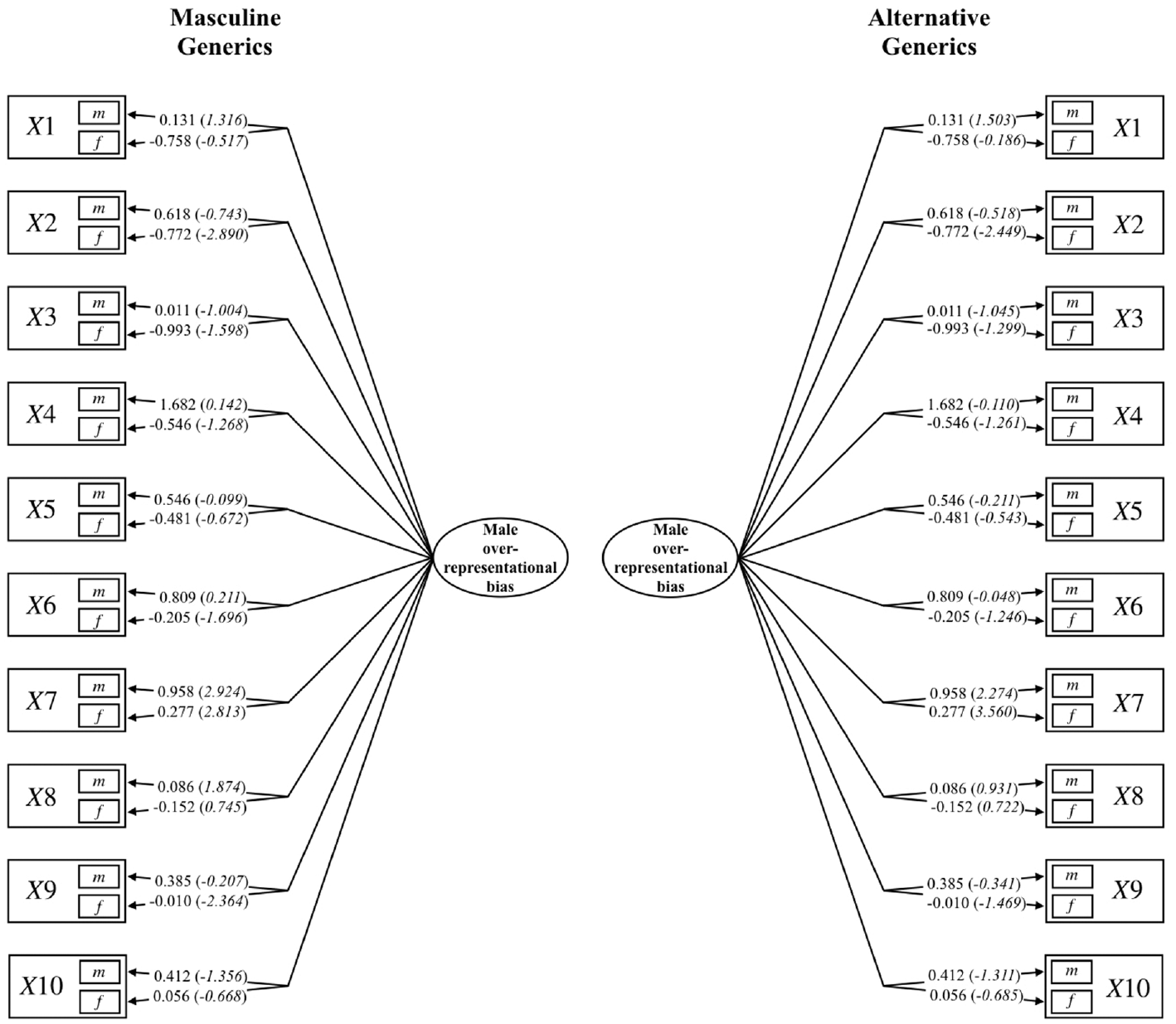
Path diagram of the fitted model.
The item response functions in Figure 8 represent the probabilities of the categories as a function of the factor score. The solid lines correspond to the MG group, and the dotted lines stand for the AG group. Similarly to the descriptive analyses, the figure reveals not substantial differences between groups except for Items X7 and X8. Also, some small differences appeared for Items X2, X3, X6, and X9. For both Items X7 and X8, the male-category was selected more frequently in the MG group than in the AG group, suggesting that these items may contain a relevant feature that elicits a masculine stereotype.
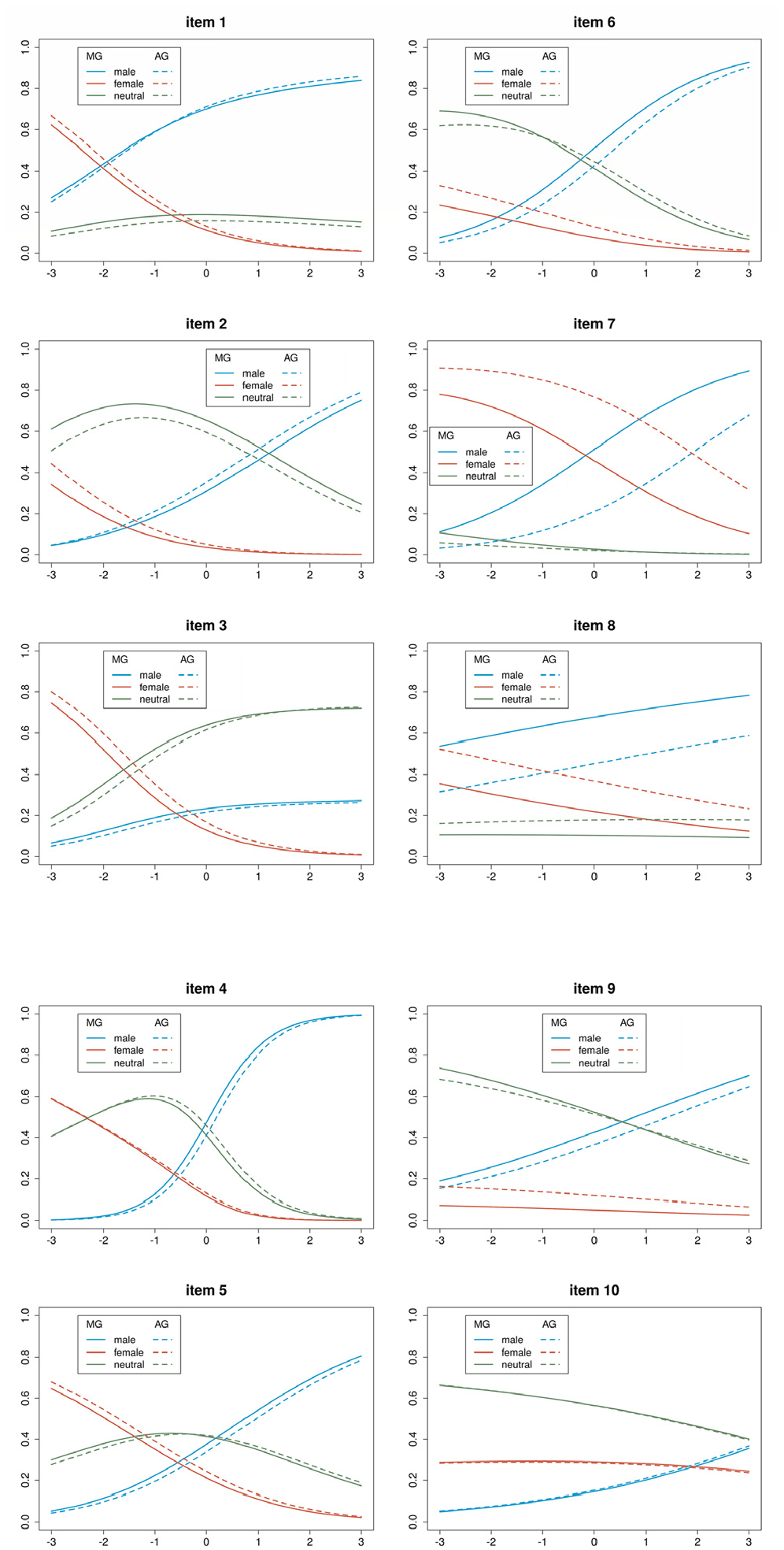
Category response functions for the MG and AG forms.
Contrast Tests
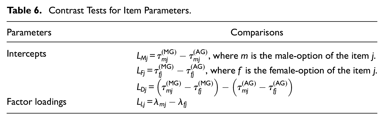
The preceding analyses indicate that there is not a general lack of invariance between the generic forms, but there could be differences related to specific items. We have applied contrast tests to further clarify these issues and compare forms item-by-item. Four contrast tests were applied to each item:
The intercept associated to the male-category in the MG form was compared to the same intercept in the AG form (
The intercept for the female-category in the MG form was compared to the same intercept in the AG form (
Difference between the intercept for the male and female categories of each item was compared across the MG and AG forms (
The loading of the male and female categories of each item was compared (
Table 6 summarizes the comparisons involved in these tests.
Contrast Tests for Item Parameters.
The total number of comparisons was 40, so the correction criteria for the Benjamini–Hochberg Type I error rate (Benjamini & Hochberg, 1995) was applied using the p.adjust() function from the stats package in R language.
The estimates of the comparisons and their corrected p values are shown in Table 7. No significant differences appeared for the comparison of the male category between the MG and AG forms (
Results of Contrast Tests for Item Parameters.
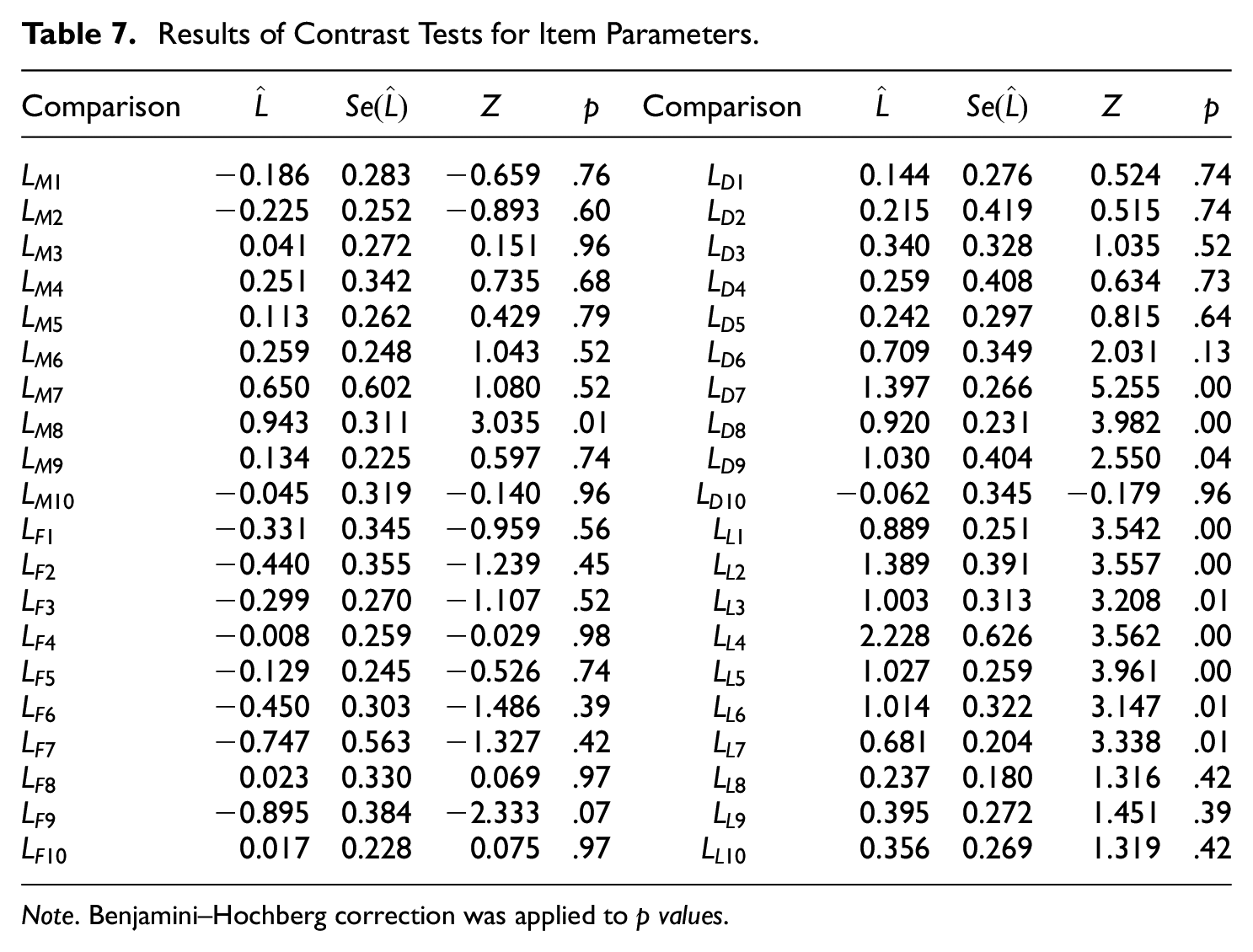
Note. Benjamini–Hochberg correction was applied to p values.
The comparison between the factor loadings of the male and female categories of each item (
Multiple-Indicator Multiple-Cause Model: Gender and Age
The MIMIC model regressed factor score on gender and age. The analysis was run for the three levels of MIMIC invariance described in the section “Multigroup Factor Analysis for Nominal Data and Levels of Invariance.” The likelihood-ratio chi-square statistics were nonsignificant, and the simplest model of invariance of slopes and intercepts was retained. This conclusion is supported also by the AIC, BIC and BICc. The results appear in Table 8.
Goodness-of-fit Indices for the MIMIC Model With and Without Invariance Between Forms.
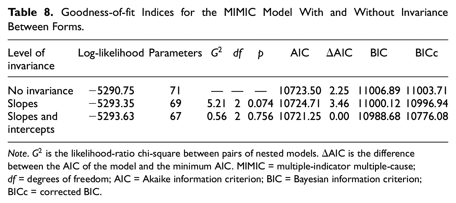
Note.
Regarding the model of invariance, the slope for age was −0.027 (
Conclusions of the Empirical Study
The MNCM allowed us to reach several substantive conclusions about the SGS. First, this model enabled us to study the dimensionality of the SGS, suggesting a one-factor model that can serve as evidence of construct validity. Second, the hypothesis of factorial invariance for both generic forms of the questionnaire (MG and AG) was not rejected on the basis of our analyses. The factorial structure includes a latent factor, which can be interpreted as the male overrepresentational bias. Indeed, factor loadings remained unchanged between forms, indicating that the relation between categories and the latent factor is not altered by the generic form, as stated in Hypothesis 1. However, the intercepts of the categories showed differences for some specific items because of a different response frequency from one form to another. These differences are related to stereotypically masculine activities, which were selected more frequently when the item is written in MG, thus retaining our Hypothesis 2. These results conform with the theory supporting the SGS. In addition, the MNCM provides an alternative approach to the study of invariance that has allowed drawing substantive conclusions regarding the initial hypotheses.
Contrast tests provided more detailed item-by-item information about the differences between the forms of the questionnaire. The simulation study has shown that increased statistical power is achieved when comparing the differences between the two item intercepts from one form to another. The analysis showed little differences between the generic forms, except for three items: X7, X8, and X9. This could be related to the fact that these items were designed based on gender roles (i.e., “beliefs about the activities considered more appropriate for men and women”López-Sáez et al., 2008, p. 610), whereas the first five represented differences between gender traits (i.e., psychological characteristics expected for each gender). From a substantive point of view, these differences between situations that represent roles and traits could be decisive in testing the effect of the use of generics in the situations presented in the SJT. These results are in line with the independence found between these two gender-stereotype components in López-Sáez et al. (2008). However, it was not among the objectives of this work to deepen the study of the differences between these two social aspects, and future research will be necessary to draw more concrete conclusions about this potential phenomenon. Another interesting fact to highlight in this analysis is that the sign of the estimates among male-categories is positive for most of the items, whereas for the female-categories, it is negative. This indicates that, in general, the male-categories are more frequently selected than the female-categories in the MG as compared to the AG form. These results suggest that the use of AG reduces stereotypically male expectations of mixed groups and are congruent with previous research on this topic (e.g., Kaufmann & Bohner, 2014).
Item-by-item analyses of factor loadings revealed a clear pattern. The slope of the male-category is higher than that of the female-category for all the items. Then, the latent factor could be conceptualized as a continuum whose ends range from preference for stereotypically female expectations for the group presented in the item (low factor score) to preference for stereotypically male expectations (high factor score). These conclusions can be interpreted as a source of construct validity evidence, as this description appropriately illustrates what was intended to be measured: male overrepresentational bias.
Finally, the part of the MIMIC model does not render significant results. No evidence of age- or gender-related differences are found in male overrepresentational bias. Regarding the covariate age, this could probably be due to a rather homogeneous sample, with ages between 17 and 30 years old. Furthermore, the application of the questionnaire via internet may also induce a selection bias by excluding participants with a lower educational level or fewer technological resources. Moreover, the linguistic use of AG is somewhat more frequent among young and educated people. A more comprehensive study would have an explicit focus on collecting participants with a variety of ages and educational levels. However, we are not aware of previous empirical findings about these issues, as the vast majority of studies in this field are based on samples of students. Regarding the lack of a significant gender effect, previous evidence is diverse. Works such as those by Merritt and Kok (1995) and Nissen (2013) did not record significant differences between genders in their respective tests of the influence of MG, whereas Hamilton (1988) and Kaufmann and Bohner (2014) did find them. For these latter authors, the explanation of these differences refers to the bias “People = Me” described by Silveira (1980), which could explain that men, in addition to the bias “People = Men,” manifested a higher male overrepresentation in mixed groups. In any case, it remains to be seen if these differences could appear in other AG not covered in this study, such as the generic with or with “-e,” which are increasingly used nowadays.
Discussion
This article addresses the problem of how to factor analyze the nominal responses originated from SJTs. A SJT presents a hypothetical scenario and a list of actions, and the individuals are asked to select their most likely action for that scenario. Because actions have no explicit order, the item generates nominal responses consisting of the actions selected by the individuals. We present procedures based on the MNCM (Revuelta et al., 2020), which is a multidimensional extension of the nominal categories model by Bock. The MNCM allows the analysis of the factorial structure for item responses that do not have an explicit order, as is the case of a SJT. Previous research has addressed the problem of factor analyzing nominal data in SJTs but has not considered the nominal categories model in the multidimensional case. The article also demonstrates the application of the MNCM in exploratory and multigroup factor analysis from the nominal data provided by an SJT.
We present the results of two studies. First, a simulation study is conducted to investigate the statistical properties of the inferential methods. The likelihood-ratio chi-square, AIC, BIC, and BICc statistics showed good results in the recovery of the invariance level of the simulated data. However, the chi-square statistic was too liberal and, in practice, useless for estimating the number of factors for the MNCM. Based on these findings we recommend the use of the indices AIC, BIC, and BICc, which do not share this problem and, for the time being, can be used to guide the selection of the number of factors.
The simulation study is focused on investigating how the goodness-of-fit statistics behave depending on the magnitude of the difference between the item parameters in the two groups. However, the simulating model is one-dimensional in all the conditions. One topic that requires further investigation is to compare results for simulating models of different dimensionality and factorial structure.
The second study is a real data example that serves as an illustration of how the MNCM can be used to factor analyze nominal responses from an SJT about gender stereotypes. The purpose of the study is to investigate latent dimensionality and to test hypotheses about the factorial structure and parameter values. Results of exploratory analyses showed that responses to the SJT are associated to a single latent factor. Concerning the analysis of the factorial invariance of the questionnaire, consisting of the comparison of the factor structure in two groups of individuals who received a different test form, the results supported the weak invariance level. From a substantive point of view, the procedure allowed us to draw conclusions concerning the use of generics and their relation with stereotypically expectations.
The contribution of the article is largely based on its focus on the SJT and the consideration of the MNCM to study its dimensionality. Previous research has focused only on the assignation of arbitrary scores to the response categories of an SJT, assuming that these scores are suitable for defining the dimensions of the SJT. A notable step further is that of Zu and Kyllonen (2018), who consider the use of a one-dimensional nominal categories model for SJT. To our knowledge, the extension to the multidimensional model and multigroup designs has not been attempted before. Future research should continue investigating the applicability of the MNCM to other item formats. For instance, multiple-choice items that also generate nominal responses could be analyzed using the same procedures described here.
The main challenge with nominal data is that several response categories are grouped together to create an item, and the parameters of the categories are interpreted in relation to the other categories of the same item instead of comparing them to the parameters of the other items. Additional investigation is necessary to determine how the item parameters of the MNCM can be compared across items.
We chose the Mplus computer program to run all these analyses because of its widespread use for structural models. Notwithstanding, more research about Bayesian methods for the nominal model (Revuelta & Ximénez, 2017) would be welcome, due to the current relative scarcity of model-fit techniques in the classical framework. For example, Bayesian methods are applicable to monitoring the posterior distribution of goodness-of-fit statistics that are not implemented in Mplus. We are aware that the Bayesian analyses require computer coding using languages such as JAGS (Plummer, 2003) or RStan (Stan Development Team, 2018), which are not routinely used by many applied investigators. Therefore, in this article, we limited our analyses to the possibilities provided by a computer program of general usage. We hope that in the near future this popular software also considers including the Bayesian procedures for the nominal model. We also hope that this research provides additional information to assist researchers when conducting the task of fitting latent variable models to nominal data.
Supplemental Material
sj-pdf-1-epm-10.1177_0013164421994321 – Supplemental material for Nominal Factor Analysis of Situational Judgment Tests: Evaluation of Latent Dimensionality and Factorial Invariance
Supplemental material, sj-pdf-1-epm-10.1177_0013164421994321 for Nominal Factor Analysis of Situational Judgment Tests: Evaluation of Latent Dimensionality and Factorial Invariance by Javier Revuelta, Alicia Franco-Martínez and Carmen Ximénez in Educational and Psychological Measurement
Footnotes
Declaration of Conflicting Interests
The author(s) declared no potential conflicts of interest with respect to the research, authorship, and/or publication of this article.
Funding
The author(s) disclosed receipt of the following financial support for the research, authorship, and/or publication of this article: This research was supported by the grant PGC2018-093838-B-I00 from the Spanish Ministerio de Ciencia, Innovacion y Universidades. Simulations have been run using the resources of the Center for Scientic Computation (Centro de Computacion Cientifica, CCC-UAM) at the UAM.
Supplemental Material
Supplemental material for this article is available online.
References
Supplementary Material
Please find the following supplemental material available below.
For Open Access articles published under a Creative Commons License, all supplemental material carries the same license as the article it is associated with.
For non-Open Access articles published, all supplemental material carries a non-exclusive license, and permission requests for re-use of supplemental material or any part of supplemental material shall be sent directly to the copyright owner as specified in the copyright notice associated with the article.