An Illustration of an IRTree Model for Disengagement

Abstract

Low-stakes test performance commonly reflects examinee ability and effort. Examinees exhibiting low effort may be identified through rapid guessing behavior throughout an assessment. There has been a plethora of methods proposed to adjust scores once rapid guesses have been identified, but these have been plagued by strong assumptions or the removal of examinees. In this study, we illustrate how an IRTree model can be used to adjust examinee ability for rapid guessing behavior. Our approach is flexible as it does not assume independence between rapid guessing behavior and the trait of interest (e.g., ability) nor does it necessitate the removal of examinees who engage in rapid guessing. In addition, our method uniquely allows for the simultaneous modeling of a disengagement latent trait in addition to the trait of interest. The results indicate the model is quite useful for estimating individual differences among examinees in the disengagement latent trait and in providing more precise measurement of examinee ability relative to models ignoring rapid guesses or accommodating it in different ways. A simulation study reveals that our model results in less biased estimates of the trait of interest for individuals with rapid responses, regardless of sample size and rapid response rate in the sample. We conclude with a discussion of extensions of the model and directions for future research.

Keywords

IRTree disengagement rapid guessing effort-moderated

Introduction

In addition to examinee ability, test performance can reflect examinee effort (e.g., Wise & DeMars, 2005). The contaminating effect of effort on scores is of particular concern in low-stakes testing, where there are little to no personal consequences to examinee performance. Examinee effort, or an examinee’s willingness to devote energy toward answering items to the best of their ability, confounds score interpretations, and attempts must be made to mitigate its influence and adjust scores for its effects (American Educational Research Association [AERA] et al., 2014). As a consequence, several methods have been proposed for measuring effort and adjusting scores. The present study adds to the collection of methods by introducing the use of an IRTree model to simultaneously measure two latent variables: disengagement (i.e., non-effortful behavior) and the trait of interest (TOI). In addition to simultaneously estimating both latent traits, the model adjusts scores on the TOI for examinee differences in effort. The purpose of the present study is to describe how an IRTree model can be used to accomplish these goals, consider its advantages over other approaches, provide an illustrative example of its use, and consider parameter recovery of the model using simulation techniques. Because our application uses Rapid Guessing (RG) indices as indicators of examinee disengagement, we begin with an overview of RG indices before describing the model and providing an illustrative example and simulation study.

RG Indices

To identify non-effortful behavior at the item level, many practitioners and researchers establish time thresholds that specify a point on the item response time continuum where examinees who respond quicker than the threshold are assumed to be exhibiting non-effortful behavior (e.g., Wise & Kong, 2005). Rapid guesses (item responses when item response times are less than the threshold) are assumed to be non-effortful and indeed, several studies support inferring non-effortful behavior when responses are rapid (Wise, 2015). Responses recorded in times longer than the threshold are more complicated to interpret as they may be due to effortful or non-effortful behavior (Wise & Smith, 2011). Although the resulting indices from this dichotomization of item response time are often called Solution Behavior (SB) indices (with values of 1 for responses at or above the threshold and 0 for those below), we use the term RG indices (with values of 0 for responses at or above the threshold and 1 for those below), given the more straightforward interpretation of response times below the threshold.

The dichotomization of item response time to create RG indices for each item is popular but limited in that it can only distinguish one kind of non-effortful behavior from all other behavior. The popularity of the method is likely attributable to some of its advantages over other methods, particularly those relying on examinees’ self-reports of their own levels of effort. One advantage is that item response time can be collected at the item level without involving the examinee or extending testing time. Another advantage is the simplicity of the computation of RG indices. Once thresholds are established, a simple comparison of item response times to the thresholds is needed to create the indices. The establishment of the thresholds is needed prior to this step and can be accomplished using a variety of methods (Rios & Deng, 2021), with some being easier to implement than others. However, because minimal differences have been found across methods (Kong et al., 2007; Rios & Deng, 2021), practitioners can use whatever method is best aligned with their skill set.

Another possible reason why RG indices are popular is the straightforward interpretation of the indices themselves and other indices created from them. For instance, RG indices can be averaged across items, with the resulting index¹ representing the proportion of items on which the examinee rapidly responded (Wise & Kong, 2005). The index can be used to represent each examinee’s level of disengagement on the test holistically and is often summarized across examinees to understand typical levels and variability across examinees in disengagement. Averaging RG indices for each item is also common, with the resulting indices indicating the proportion of examinees rapidly responding on each item (Wise, 2006). When the RG indices are averaged across items for a given examinee or averaged across examinees for a given item, the resulting values are the same as the observed total score and item difficulties, respectively, obtained using a classical test theory approach to measuring disengagement with the RG indices as indicators.

Use of RG Indices to Adjust Scores

RG indices have been used in a variety of ways to adjust scores on the TOI. For instance, an approach known as motivation filtering deletes examinees with high levels of rapid guessing from the data set (Sundre & Wise, 2003). Motivation filtering begins by first, obtaining the average of the RG indices across items, and second, deleting from the data examinees with averages above a certain value. For instance, if a cutoff of .10 were implemented, any examinee rapidly guessing on more than 10% of the items would be removed from the data. Summaries of test results are then based on the remaining examinees; thus, in motivation filtering the overall results are “adjusted.” Although easy to implement and explain, motivation filtering makes the strong assumption that rapid response behavior is unrelated to the TOI. If this assumption is not satisfied, the adjusted results are biased and not trustworthy. Recent work by Deribo et al. (2021) found that rapid guessing depends on the examinee’s true response had they not rapidly guessed, indicating there is an underlying relationship between rapid guessing behavior and TOI. This result supports an ability–effort relationship found by Rios et al. (2017) and Wise et al. (2009), contrary to earlier studies with no support for this relationship (e.g., Sundre & Wise, 2003; Wise & Kong, 2005).

Other approaches for adjusting scores using RG indices involve converting the item responses on which examinees rapidly guessed to missing and then employing modern missing data techniques, such as multiple imputation or maximum likelihood estimation. For example, in the effort-moderated item response theory (IRT) model (Wise & DeMars, 2006), an IRT model for the TOI is estimated using the modern missing data technique of maximum likelihood estimation after item responses that are rapid guesses are converted to missing. The assumption² regarding the relationship between rapid guessing and the TOI is less strong than in motivation filtering and more likely to be satisfied in practice. For this reason, modern missing data approaches are recommended over motivation filtering. Another advantage of these approaches over motivation filtering is the adjustment of TOI scores for individual examinees. Motivation filtering removes examinees from the data with a predetermined level of problematic rapid guessing; these examinees will not obtain a TOI estimate and the TOI for examinees who are retained, but still rapidly guessed on items, will remain unadjusted. In contrast, approaches based on modern missing data techniques retain all examinees in the data and provide TOI estimates adjusted for rapid guessing behavior.

Desirable methods for adjusting scores for rapid guessing behavior are those that: (a) do not assume independence between rapid guessing and the TOI, (b) do not remove examinees from the data, and (c) do adjust scores for individual examinees who engage in rapid guessing behavior. As aforementioned, methods utilizing RG indices exist with these characteristics (e.g., effort-moderated IRT model). We propose yet another method that has the added advantage of modeling the latent trait of disengagement while simultaneously modeling the latent TOI, which is adjusted for rapid guessing. Modeling the latent trait of disengagement using RG indices within an IRT framework is advantageous over the classical test theory approach, which yields parameter estimates that are sample and test specific.

IRTree Model for Disengagement

IRTrees (De Boeck & Partchev, 2012) are multidimensional extensions of item response models, allowing practitioners greater flexibility in modeling response processes. By explicitly modeling the sequential decision-making process used by examinees, IRTrees have been applied to modeling multiple-choice answer change behavior (Jeon et al., 2017), rubric rater scoring (Myers et al., 2020), survey respondents’ response styles (Spratto et al., 2021), and question skipping behavior (Debeer et al., 2017). Each IRTree model is defined by the hypothesized stages of item answer behavior.

For this application of an IRTree, all examinee responses for each item are classified as a rapid guess (i.e., RG response), a correct response, or an incorrect response. Although RG responses may be correct or incorrect, we assume they do not contribute information to the TOI and are therefore classified distinctly. The IRTree model for disengagement hypothesizes response behavior as involving two stages, as shown in Figure 1. A non-effortful response, such as a rapid guess as determined using a time threshold approach, leads to a terminal node after Stage 1. 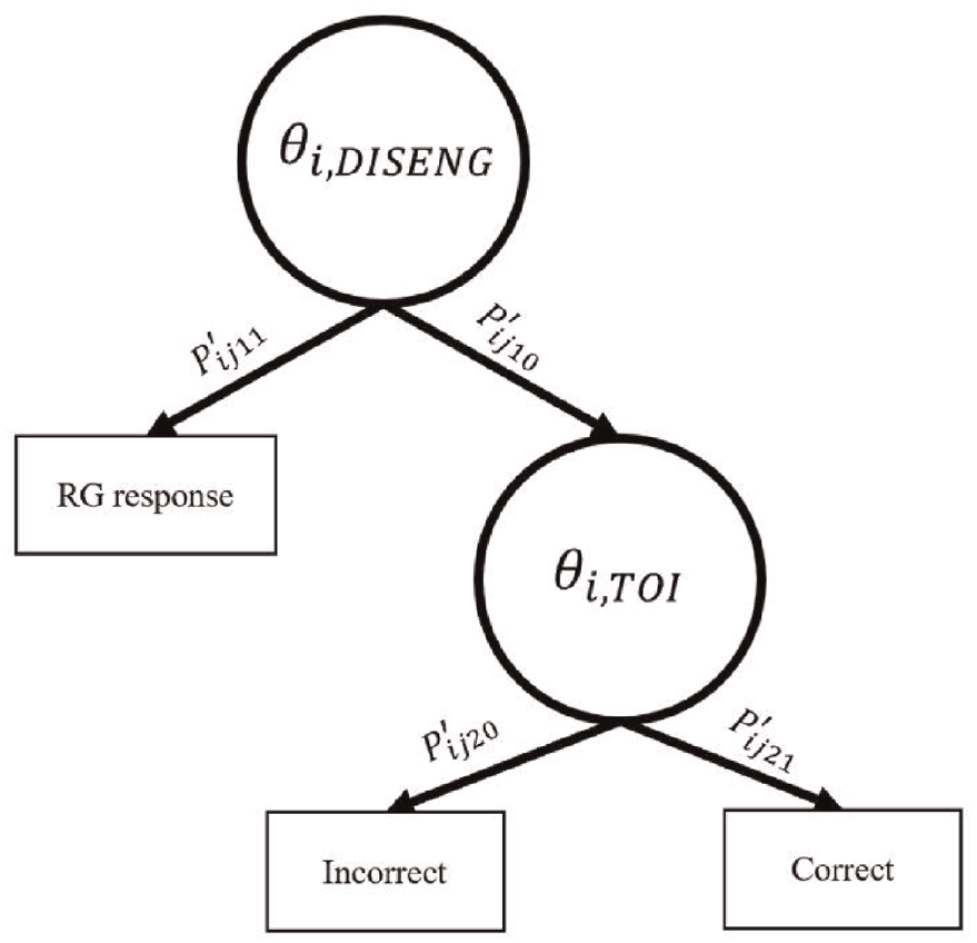Stage 1, whether a respondent engages in rapid guessing, is driven by latent trait $θ_{i, DISENG}$ , where higher values indicate higher tendencies toward rapid guessing behavior. Stage 2, whether a correct answer is selected, is a function of the underlying latent TOI, $θ_{i, TOI}$ , where higher values indicate higher ability.

Figure 1.

IRTree Model for Disengagement.

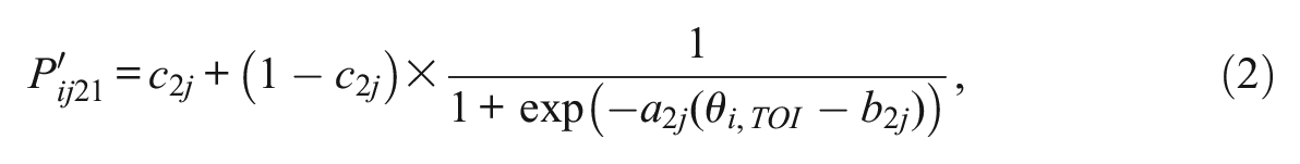
As shown in Figure 1, each stage is a dichotomous split. Therefore, we model each stage using a dichotomous unidimensional IRT model. In Stage 1, rapid guessing behavior is modeled as a function of the DISENG trait using a 1-parameter logistic (1-PL) model. In Stage 2, we model the probability of a correct response using the 3-parameter logistic (3-PL) model. For item j, the probability of a value of 1 at Stage k for the individual i is $P_{ijk 1}'$ . For Stage 1, the probability of a rapid guess on item j for examinee i with $θ_{i, DISENG}$ is

P_{i j 11^{'}} = \frac{1}{1 + \exp (- a_{1} (θ_{i, D I S E N G} - b_{1 j}))},

(1)

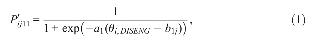
and the probability of a non-rapid guess is $P_{ij 10}' = 1 - P_{ij 11}'$ . Higher $θ_{i, DISENG}$ values lead to higher likelihood of engaging in rapid guessing. These tendencies, however, interact with item characteristics, expressed through the Stage 1 specific item parameters. For Stage 2, the probability of a correct response on item j for examinee i with latent ability $θ_{i, TOI}$ is

P_{ij 21}' = c_{2 j} + (1 - c_{2 j}) \times \frac{1}{1 + \exp (- a_{2 j} (θ_{i, TOI} - b_{2 j}))},

(2)

and the probability of an incorrect response is $P_{ij 20}' = 1 - P_{ij 21}'$ .

The three types of item responses, which include a RG response or an incorrect/correct response for a non-RG response, have the following probabilities:

\begin{matrix} P (RG response) = P_{ij 11}' \\ P (Incorrect) = P_{ij 10}' \times P_{ij 20}' \\ P (Correct) = P_{ij 10}' \times P_{ij 21}' \end{matrix}

(3)

Stage-specific item parameters include $a_{1}, b_{1 j}, a_{2 j}, b_{2 j}$ , and $c_{2 j}$ . For Stage 1, $a_{1}$ represents the common item discrimination on the latent trait of disengagement and $b_{1 j}$ represents stage-specific item difficulty. Lower difficulty values suggest that even examinees with low levels of the DISENG latent trait are likely to rapidly guess to the item; if item difficulty is high, higher levels of the DISENG latent trait are needed to rapidly guess. For Stage 2, $a_{2 j}$ represents the item discrimination on the TOI, $b_{2 j}$ is the item difficulty with respect to the TOI, and $c_{2 j}$ is the pseudo-guessing parameter.³ The interpretation of the item parameters at Stage 2 are the same as in any application of the 3PL to the latent TOI.

Novel to this model is the ability to estimate the relationship between the disengagement trait and the TOI. Unlike the effort-moderated model, our model assumes the probability of rapidly guessing is a function of a continuous latent trait. As noted by Liu et al. (2019), this allows further investigation of the causes of disengagement. In our application of the model, we assume the two latent traits follow a multivariate normal distribution,

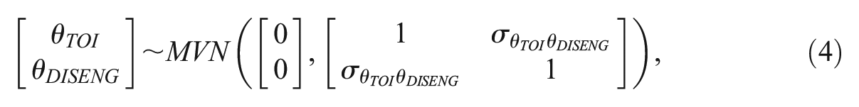
[\begin{matrix} θ_{TOI} \\ θ_{DISENG} \end{matrix}] ~ MVN ([\begin{matrix} 0 \\ 0 \end{matrix}], [\begin{matrix} 1 & σ_{θ_{TOI} θ_{DISENG}} \\ σ_{θ_{TOI} θ_{DISENG}} & 1 \end{matrix}]),

(4)

with $σ_{θ_{TOI} θ_{DISENG}}$ representing the correlation between the traits.

The purpose of this two-part study is to fit the IRTree model for disengagement to low-stakes testing data. In Part 1, we illustrate model estimation and interpretation using an empirical data set. To highlight the benefits of the model, results are also compared with a 3-PL model fit to the same data without accounting for which responses were rapid guesses. In Part 2, we examine the bias of the TOI trait estimates using simulation, also with a comparison to bias in the TOI under the 3-PL when rapid guessing is present.

Part 1—Empirical Study

Method

Sample and Procedures

To exemplify this model, we use scores on a 40-item multiple-choice oral communication knowledge assessment administered in Spring 2021. With the help of assessment specialists, the test is developed by subject matter experts consisting of faculty who teach the content to first-year students at a mid-Atlantic university. There were four to five response options for each item, for which only one response could be selected and one response was correct. Scores from the test are used to satisfy institutional assessment requirements and for outcomes assessment purposes only. In our study, we assessed a random sample of students with between 45 and 70 credit hours (i.e., sophomore and juniors) who had completed the relevant coursework. For students in our sample, the assessment was low stakes, meaning there was no personal consequence for performing well or poorly on the assessment. Students were encouraged to try, but motivation remained a concern. Therefore, effort must be taken into account when interpreting the results, making the data a suitable application of the IRTree model for disengagement. After completing the oral communication assessment, each student completed self-report items on the effort subscale from the Student Opinion Survey (Thelk et al., 2009) as a holistic measure of motivation.

The 447 examinees completed the assessment in an average of 13 minutes with a standard deviation of about 9 minutes. On average, students answered 26.82 items correctly with a standard deviation of 8.8. Effort scores indicated moderate effort by the typical examinee, with an average of 3.57 (SD = .65) on a scale with 1 representing low effort and 5 being high effort.

To apply the IRTree model, we first determined thresholds for each item to identify rapid guessing. We applied a conservative Normative Threshold method with thresholds equal to 10% of the mean item response time. Item response times for all respondents are displayed in the top panel of Figure 2, with the quickest (lowest) response times highlighted in the bottom panel to display mean response time and established thresholds. Across all items, the average threshold time was 1.92 seconds with the highest threshold being only 3.43 seconds. These modest threshold values were set purposely low to identify responses where it was objectively clear that the examinees were rapidly guessing. With the thresholds established, RG responses were then calculated for each item and examinee. Rapid guessing rates varied across items, with most rapid guesses occurring in the middle third of the test. Rapid guessers have much lower accuracy rates across items than non-rapid guessers, as displayed in Figure 3. Among examinees, the average number of RG responses was 4 with a standard deviation of 8.95. As shown in Figure 4, 339 (75.8%) examinees did not rapidly guess on any items, 13 (2.9%) examinees rapidly guessed on 1 item, and 1 (0.2%) examinee rapidly guessed on 35 items.

Figure 2.

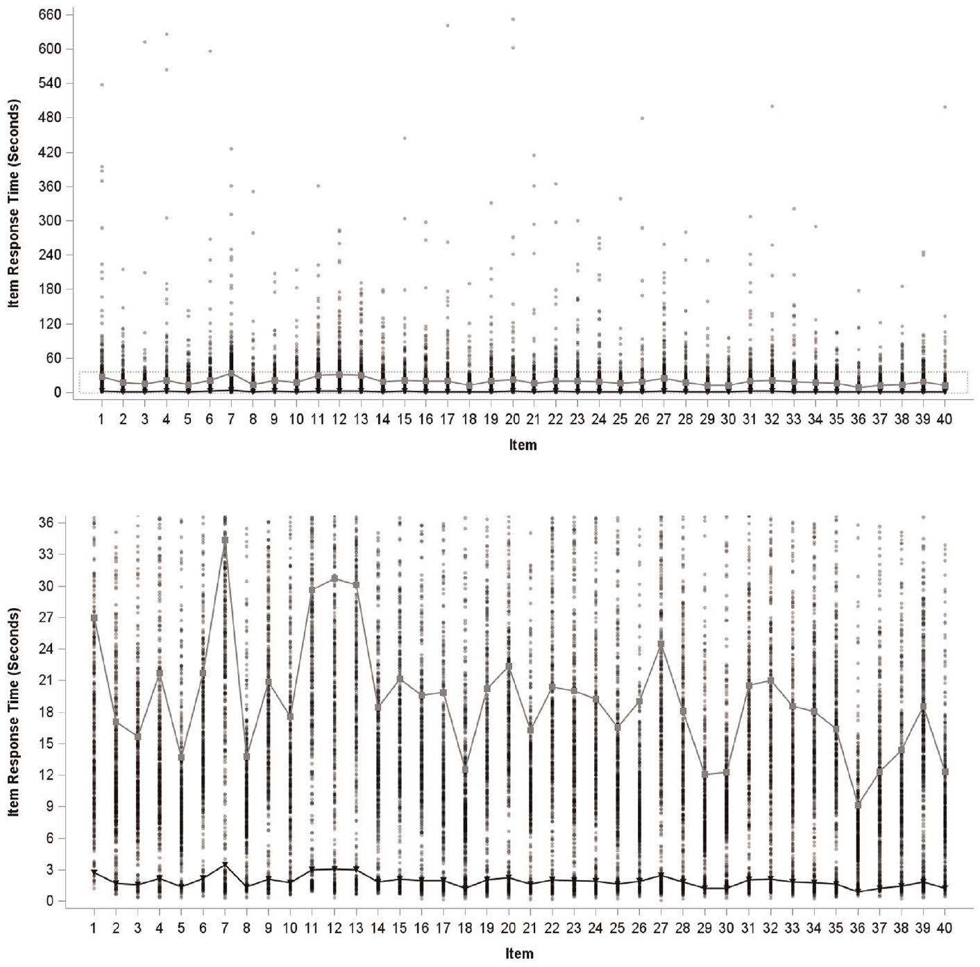
Distribution of Item Response Times With Mean Response Time (Gray) and Threshold (Black).

Figure 3.

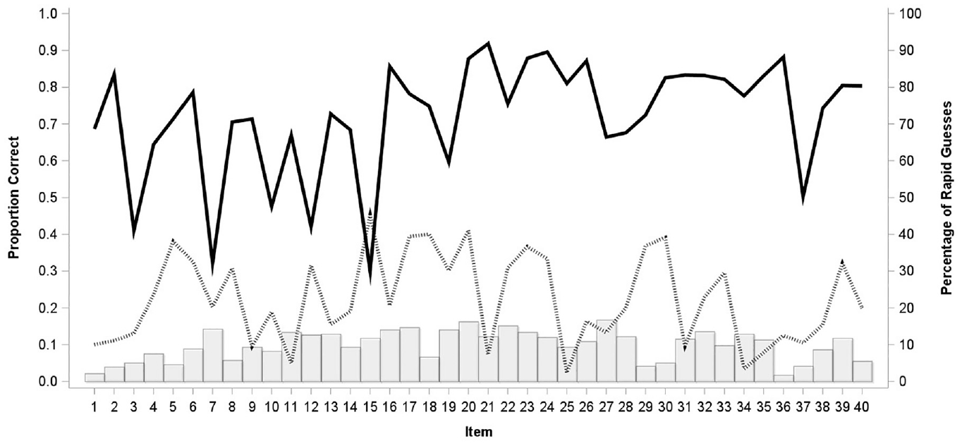
The Proportion of Rapid Guess and Accuracy Rates for Rapid Guessers and Non-Rapid Guessers Among Items.

Figure 4.

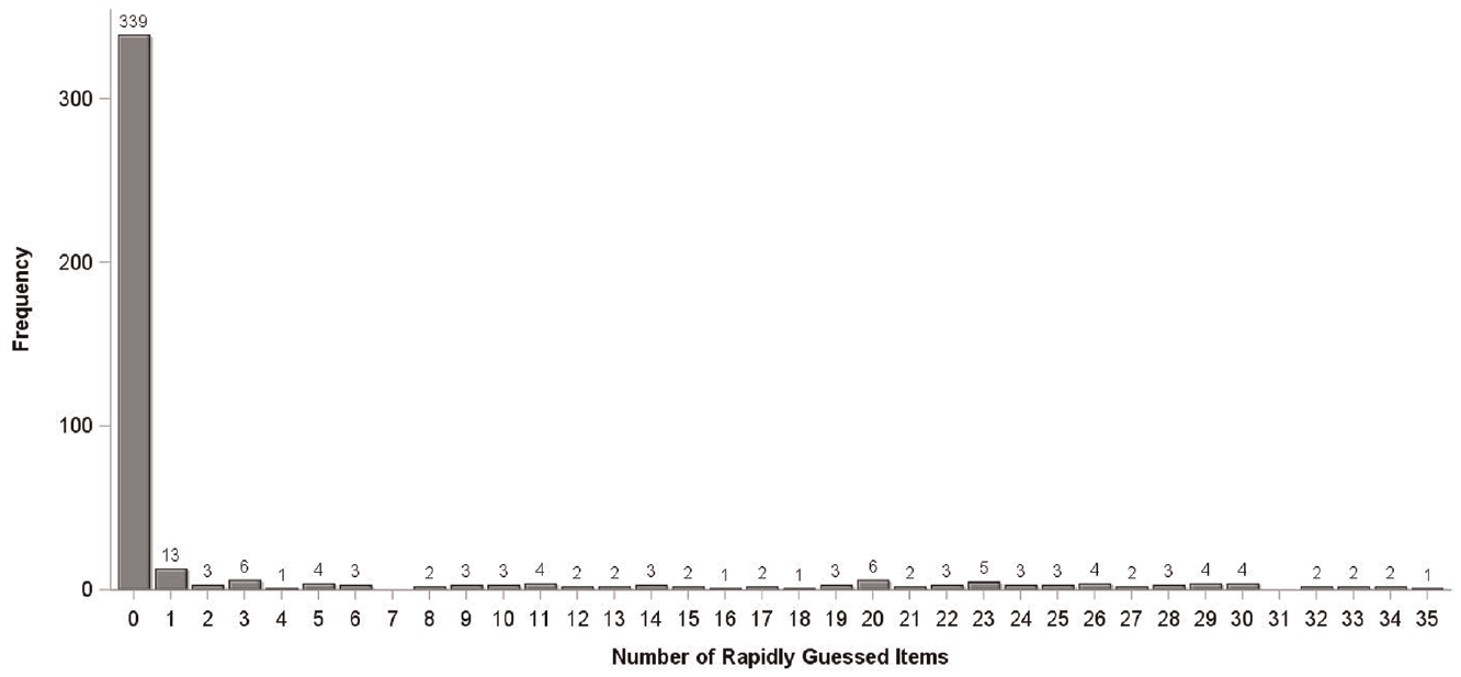
Distribution of Rapid Guesses as Determined Using the 10% of Mean Normative Threshold Approach.

Models and Estimation

To illustrate the model, we fit the IRTree and the traditional 3-PL model to examinee responses. To fit the models, a Bayesian Framework using the Markov chain Monte Carlo (MCMC) procedure in SAS (SAS Institute Inc., 2018) was utilized. In a Bayesian framework, the likelihood is combined with the prior distribution for the parameters to form a posterior distribution used for interpretation. For both the IRTree and 3-PL models, semi-informative priors were used for discrimination item parameters and noninformative priors were used for difficulty and pseudo-guessing parameters:

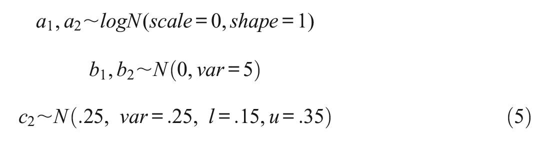
\begin{matrix} a_{1}, a_{2} ~ logN (scale = 0, shape = 1) \\ b_{1}, b_{2} ~ N (0, var = 5) \\ c_{2} ~ N (. 25, var = . 25, l = . 15, u = . 35) \end{matrix}

(5)

Due to literature exemplifying both support for and lack of support for a relationship between the traits, we include uncertainty in the correlation by assuming a hyperprior normal distribution with mean 0, variance 2, upper limit 1, and lower limit −1. For the 3-PL model, we assume that the TOI follows a standard normal distribution.

To estimate parameter posterior distributions for both models, we retain 140,000 samples thinned by a factor of 10 after discarding the first 10,000 iterations as burn-in. Convergence was assessed using trace plots, autocorrelation plots, and posterior density plots. After convergence was assured, means were retained as point estimates of model parameters with the highest posterior density (HPD) intervals providing probable ranges of parameter values.

Analysis

Item Parameter Estimates

We first compare the estimated item parameters from the 3-PL model with estimated parameters from Stage 2 in the IRTree model. In addition to considering how parameters differ across models, we also consider how the results align with those of Wise and DeMars (2006) who compared item parameters obtained when fitting the 3-PL (which ignored rapid guesses) and effort-moderated IRT model (which treated rapid guesses as missing when estimating the 3-PL) to the same data. We then interpret Stage 1 parameters for the IRTree model. Due to the low prevalence of rapid guessing behavior, we expect high item difficulties in Stage 1, resulting in low information discrimination among students with low disengagement tendencies.

Trait Estimates

To inform trait interpretations, we first look at the relationship of estimated traits from the IRTree with trait estimates from the 3-PL in addition to a criterion (e.g., self-reported effort scores, total testing time), which we expect to be positively related. Following these relationships, we further discuss the disengagement trait and then exemplify the model trait adjustments using response patterns from three examinees.

Standard Error of Trait Estimates

In an MCMC framework, the standard deviation of the posterior distribution reflects the uncertainty in the estimate, comparable to the standard error of the estimate in a frequentist framework. Here we compare the standard deviation of the posterior of the TOI estimate obtained from the 3-PL and IRTree, anticipating enhanced precision under the IRTree. To eliminate Bayesian estimation as a possible explanation of our results, we then compare the relationship of the standard deviation obtained from the 3-PL and IRTree to the relationship of the standard deviation of the TOI estimate obtained from the 3-PL and the effort-moderated model, with parameters also estimated using Bayesian methods. We expect to see that our IRTree model, which treats disengagement as a predictor-like variable for the TOI, shows improved precision and the effort-moderated model, which treats rapid guesses as missing, to have less precision.

Examinee Illustration

To exemplify the differences between the IRTree model and the 3-PL, we explore three students with the same total score but different disengagement patterns. We expect to see adjustments to the TOI and differences in disengagement trait estimates across the three students due to their unique rapid guessing patterns.

Results

Item Parameter Estimates

As displayed in Figure 5, there is a strong, positive relationship between the estimated item difficulty parameters from the 3-PL and those estimated in Stage 2 of the IRTree. This result aligns with estimates found by Wise and DeMars’ (2006) effort-moderated model, where harder items (as estimated from the 3-PL) were somewhat harder and easier items (as estimated from the 3-PL) were less difficult when estimated using the IRTree. Similarly, estimated item discrimination parameters showed a strong, positive relationship between the two models, as displayed in Figure 6. This pattern was also consistent with Wise and DeMars’ (2006) application of the effort-moderated model, where there is more agreement among discrimination estimates for lower discriminating items from the 3-PL, and higher discriminating items from the 3-PL do not discriminate as highly using the IRTree.

Figure 5.

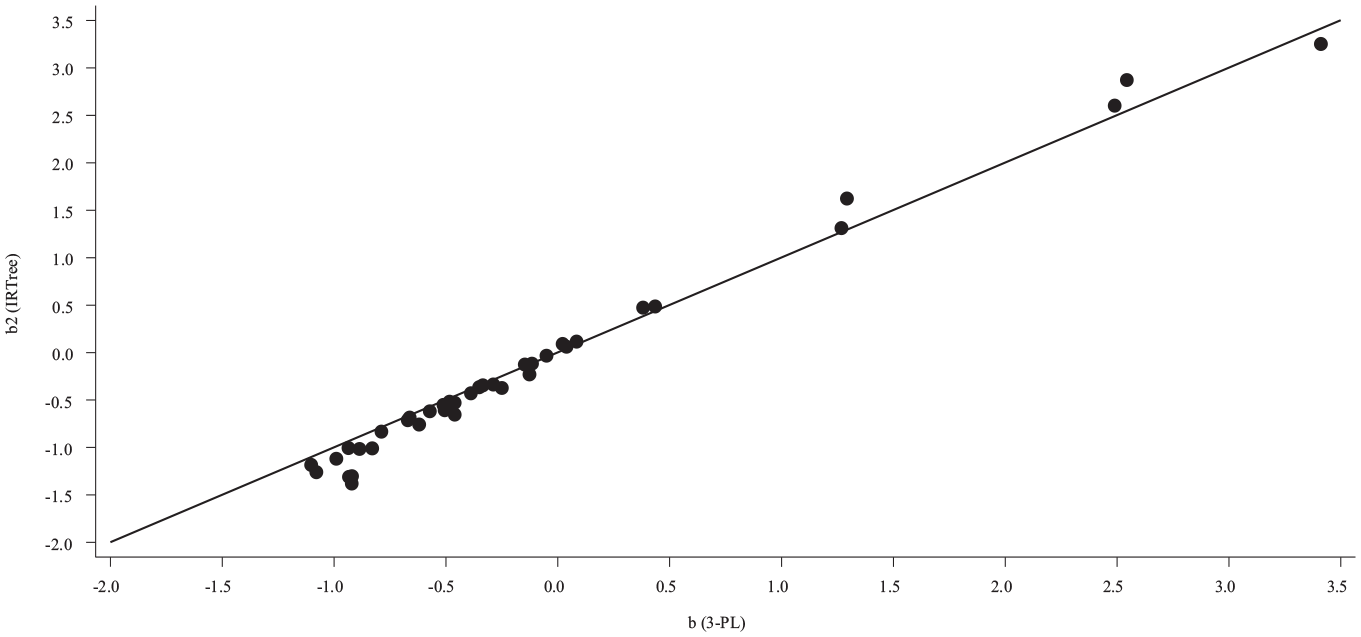
Item Difficulty Parameter Estimates from Stage 2 of the IRTree (Vertical Axis) and the 3-PL Models (Horizontal Axis).

Figure 6.

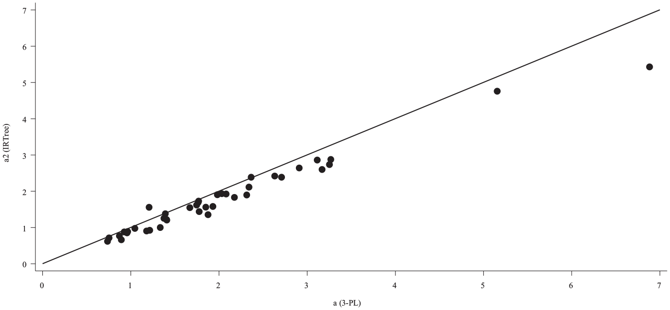
Item Discrimination Parameter Estimates from Stage 2 of the IRTree (Vertical Axis) and the 3-PL Models (Horizontal Axis).

All items exhibit strong relations with the DISENG trait as indicated by a common-item discrimination parameter mean of 4.4 [95% HPD: 3.9, 4.9]. Item difficulty means and non-symmetric HPD interval estimates from Stage 1 are presented in Figure 7. It is unlikely for a given item to lead to a rapid guess unless an examinee has a high DISENG trait value as evidenced by the high difficulty parameter estimates among the items. The high difficulty and discrimination values also indicate that we can reliably measure people with high disengagement, but are limited in how well we measure individuals with low disengagement based solely on the observation of a rapid guess. This is likely a result of the skewness in the latent trait.

Figure 7.

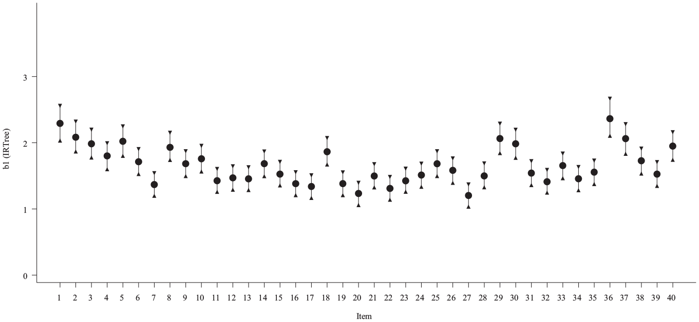
Stage 1 Threshold Parameter Mean and Highest Posterior Density Estimates.

Trait Estimates

There is a strong positive relationship between the TOI estimates under the IRTree and the 3-PL model, $r = . 99$ . Furthermore, there is a strong negative relationship between the DISENG trait and the TOI from the IRTree, $r = - . 93$ and between the DISENG trait and the TOI estimate from the 3-PL model, $r = - . 98$ . As expected, the relationship between the disengagement trait with the TOI estimate from the 3-PL is stronger than its relationship with the TOI estimate from the IRTree. This is due to individuals’ high disengagement being confounded in the TOI estimates under the 3-PL, creating a stronger negative relationship with the DISENG trait from the IRTree. Disengagement was separated out of the TOI estimate using the IRTree, resulting in a weaker relationship between the DISENG trait and the TOI from the IRTree.

There is a strong, positive relationship between sum of the RG indices for each examinee (which is a measure similar to response time effort; see Note 1) and their DISENG trait estimate, ${\hat{θ}}_{D I S E N G}$ , $r = . 83$ . Moreover, there is a strong, negative relationship between the total time taken on the assessment and DISENG trait estimates, $r = - . 82$ . Together, these indicate that the DISENG trait is capturing rapid guessing behavior as we have defined it with our RG thresholds. Furthermore, there is a strong negative relationship between the number of items identified as rapid guesses for each examinee and their TOI trait as estimated from the IRTree, $r = - . 78,$ indicating individuals with higher amounts of rapid guessing have lower ability. Respondents with higher self-reported effort scores tended to have higher TOI estimates from the 3-PL, $r = . 50$ and from the IRTree, $r = . 51$ . Finally, examinees who were less disengaged had higher self-reported effort, $r = - . 51$ , providing support that our disengagement trait is capturing effort tendencies.

Given the patterns observed in item parameter estimates, we can only be confident in reliably measuring examinees with high disengagement. As seen in Figure 8, the DISENG trait distribution is bimodal. The variation around the upper mode is likely a result of observed differences in rapid guesses. The variation around the lower mode is likely not a direct result of observable rapid guesses behavior but rather a function of the prior distribution and the estimated relationship between the TOI and disengagement. Therefore, we advise caution when looking at individual differences among DISENG estimates for this lower group as DISENG trait estimate differences are even observed among examinees who each rapidly guessed on 0 items.

Figure 8.

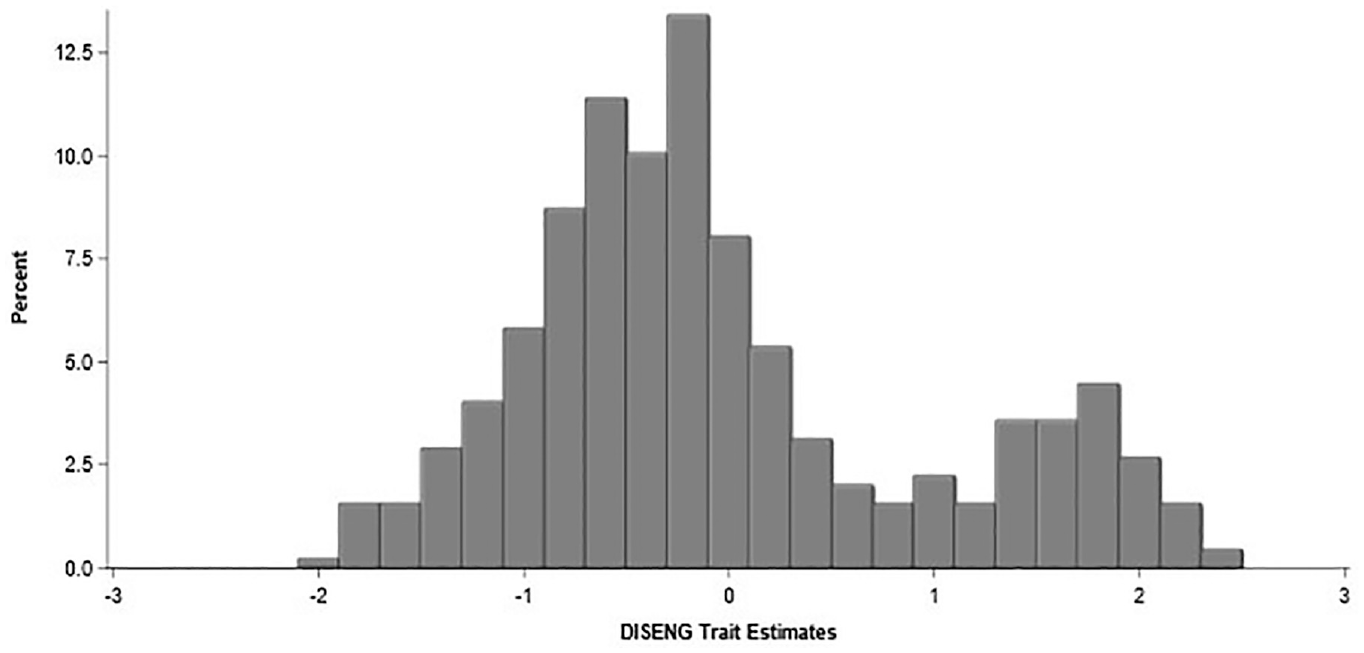
Distribution of the DISENG Trait Estimates.

Standard Error of Trait Estimates

For examinees who rapidly guessed on at least one item, there was a significant reduction in the standard deviation of trait estimates from the IRTree as compared with the 3-PL. As illustrated in Figure 9, there is a trivial difference in the standard deviation of the posterior for the TOI when examinees did not rapidly guess on any items (light gray present along x=y diagonal), but there is a significant reduction in standard deviation for individuals who rapidly guessed on 1 (gray) and 2 or more items (black), as most are located in the lower right of the plot, below the x=y diagonal.

Figure 9.

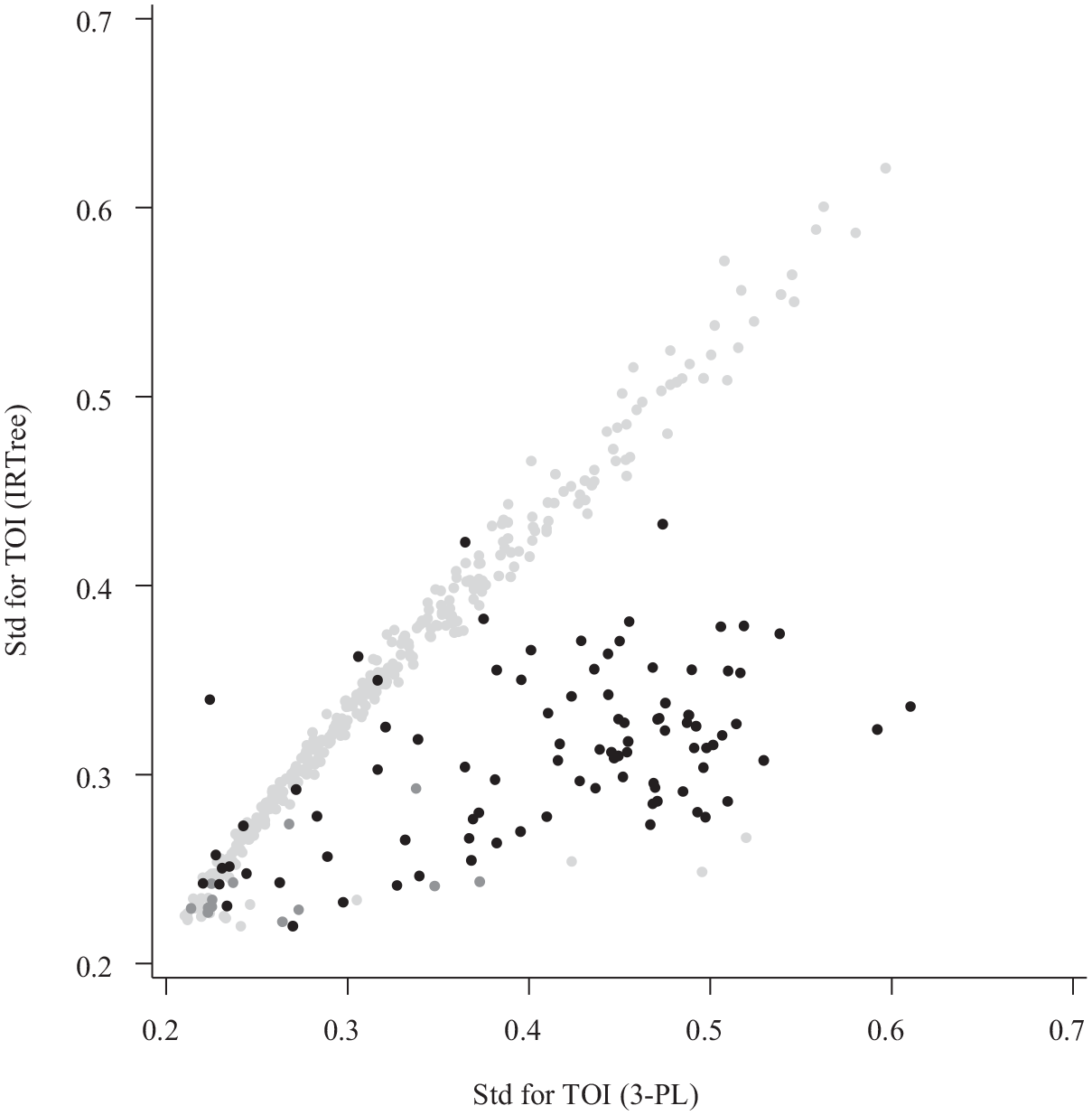
Standard Error for TOI Trait Estimates from the 3-PL and the IRTree Model.

This reduction in standard deviation is contrary to results from the effort-moderated model, where Wise and DeMars (2006) evidenced a reduction in information for the trait of interest estimates for the effort-moderated model relative to the 3-PL. Besides using different models, in our study, we use a Bayesian framework for estimation as compared with a frequentist approach in Wise and DeMars (2006). To determine whether the difference in results was due to the Bayesian approach, we fit the effort-moderated model to the data, creating a similar graph to that in Figure 9 but now with the standard deviation for TOI from the effort-moderated model on the vertical axis. The resulting pattern resembled a mirror image, where the black and gray points are reflected over the light-gray diagonal. In other words, even in a Bayesian framework, there were higher standard deviations for trait estimates from the effort-moderated model as compared to the 3-PL for individuals who rapidly guessed to at least one item. Thus, our increase in certainty for the IRTree model is not due to differences in the estimation framework.

Examinee Illustration

To illustrate the distinctions between the IRTree and the 3-PL models, we explore three students with the same total score (18), but with unique rapid guessing behavior. Student 366 rapidly guessed on 14 items, Student 322 rapidly guessed on 4 items, and Student 48 did not rapidly guess on any items. Response set profiles of Students 48, 322, and 366 are displayed in Figure 10. Of the 18 items student 366 correctly answered, four were likely due to chance given their rapid guessing behavior. Of the 18 items that student 322 answered correctly, two were likely due to chance as they were on items in which the student rapidly guessed, as identified through our Normative Threshold cut-offs.

Figure 10.

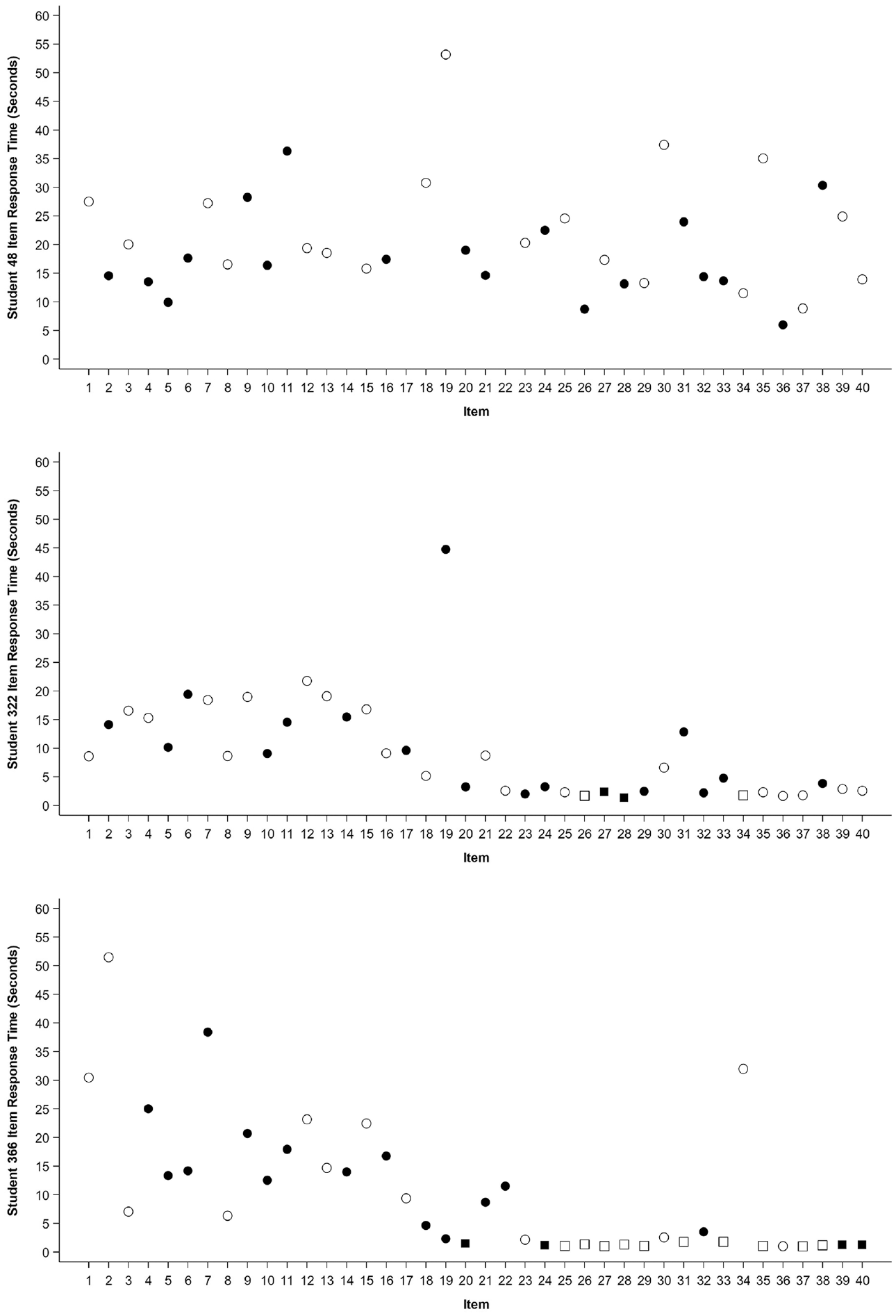
Response Profiles for Students 48, 322, and 366.

Although these three students answered the same number of items correctly, they did not answer the same exact items correctly. Thus, 3-PL model estimates, ${\hat{θ}}_{48, T O I}, {\hat{θ}}_{322, T O I}$ , and ${\hat{θ}}_{366, T O I}$ , varied as shown in Table 1. After accounting for disengagement, TOI estimates had significantly greater variation, as listed in the IRTree model column in the same table. TOI estimates of Students 366 and 322 were adjusted downward, and Student 48’s TOI estimate remained unchanged as compared with TOI estimates under the 3-PL. This is due to the DISENG trait estimate and patterns in each examinee’s response profile. For Student 366, ${\hat{θ}}_{366, D I S E N G}$ was much higher than average as the examinee exhibited rapid guessing behavior on 14 items. Although Student 322 only rapidly guessed on four items, this was still more than the average student (see Figure 4). Therefore, ${\hat{θ}}_{322, D I S E N G}$ was still higher than average.

Table 1.

Example Student Trait Estimates.

Student ID	Total Score	# Rapid Guesses	3-PL		IRTree
Student ID	Total Score	# Rapid Guesses	${\hat{θ}}_{i, T O I}$	${\hat{σ}}_{θ_{i, T O I}}$	${\hat{θ}}_{i, T O I}$	${\hat{σ}}_{θ_{i, T O I}}$	${\hat{θ}}_{i, D I S E N G}$
48	18	0	–.74	.23	–.75	.22	.41
322	18	4	–1.14	.27	–1.22	.22	1.03
366	18	14	–1.09	.36	–1.28	.30	1.44

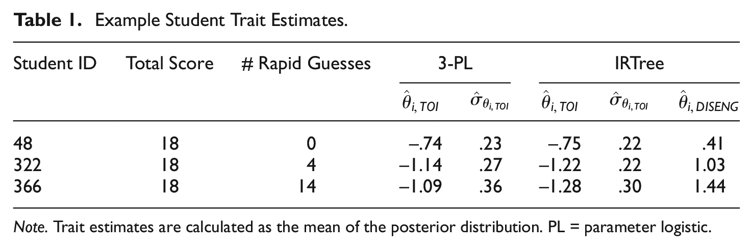
Note. Trait estimates are calculated as the mean of the posterior distribution. PL = parameter logistic.

Both Student 322 and Student 366 had a lower estimate of ability in the IRTree model as compared with the 3-PL. Since Student 322’s rapid guesses resulted in two correct items, in the IRTree model, these responses are no longer considered a function of TOI as they were in the 3-PL. Thus, the 3-PL likely overestimates TOI, which is why we see a reduction in ${\hat{θ}}_{322, T O I}$ in the IRTree model. For Student 366, four correct responses were received from rapid responses, which under the IRTree model are no longer treated as a function of the TOI. Thus, ${\hat{θ}}_{366, TOI}$ is lower under the IRTree model as compared with the 3-PL model. Since Student 48 did not rapidly respond to any items, there is no practical difference in the point estimate, ${\hat{θ}}_{48, T O I}$ , under each model.

For the two examinees who rapidly responded to at least one item, the standard deviation of the posterior for the TOI (comparable to the standard error of the estimate) from the IRTree model was lower than the standard deviation for the TOI from the 3-PL model. Across examinees, as the number of rapid guesses increases, there is a higher standard deviation of the TOI estimate from the IRTree, but this standard deviation remains lower than the standard deviation of the TOI estimated from the 3-PL.

Part 2—Simulation Study

Methods

Simulation Design

Our simulation study has a 2x2 design with item responses generated for two sample sizes (N $= 500, 2000$ ) and two RG rates (Low and High). The RG rates refer to the tendencies of the sample, not individual response sets. Thus, even when RG rates are low in the sample, simulees may be present who have rapidly responded to many items in their response set. The condition in which the sample size is 500 and the RG rate is low represents a simulated scenario most comparable to the empirical study in Part 1. For the 50 replications in each of four conditions, responses to 40 items were generated using the IRTree model to control the level of rapid responding.

Trait Generation

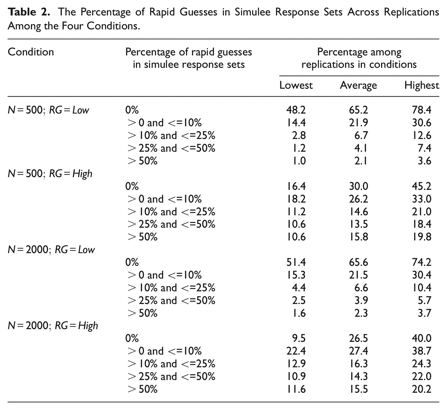
True TOI and DISENG traits were randomly selected from a multivariate normal distribution with a mean of 0 for the TOI trait, variances of 1 for both the TOI and DISENG traits, and a correlation of −.70 between the traits. To generate low RG rates, the mean of the disengagement trait in the multivariate distribution was 1 and to generate high RG rates, the disengagement trait mean was set to 2. These means, in combination with the item parameters (discussed below), were determined to create a pattern similar to the RG rates evidenced in Part 1, and a pattern of high RG rates clearly discernible from the low RG rate. The pattern of generated RG rates is summarized across replications in each of the four conditions in Table 2, where simulee response sets were categorized into five groups of rapid response behavior. For high RG rate conditions, at least 10.6% of simulees in each replication rapidly responded to at least 50% of the items. For low RG rate conditions, at most 3.7% of simulees in each replication rapidly responded to at least 50% of the items.

Table 2.

The Percentage of Rapid Guesses in Simulee Response Sets Across Replications Among the Four Conditions.

Condition	Percentage of rapid guesses in simulee response sets	Percentage among replications in conditions
Condition	Percentage of rapid guesses in simulee response sets	Lowest	Average	Highest
$N = 500;$ $RG = Low$	0%	48.2	65.2	78.4
	>0 and <=10%	14.4	21.9	30.6
	>10% and <=25%	2.8	6.7	12.6
	>25% and <=50%	1.2	4.1	7.4
	>50%	1.0	2.1	3.6
$N = 500;$ $RG = High$
	0%	16.4	30.0	45.2
	>0 and <=10%	18.2	26.2	33.0
	>10% and <=25%	11.2	14.6	21.0
	>25% and <=50%	10.6	13.5	18.4
	>50%	10.6	15.8	19.8
$N = 2000;$ $RG = Low$
	0%	51.4	65.6	74.2
	>0 and <=10%	15.3	21.5	30.4
	>10% and <=25%	4.4	6.6	10.4
	>25% and <=50%	2.5	3.9	5.7
	>50%	1.6	2.3	3.7
$N = 2000;$ $RG = High$
	0%	9.5	26.5	40.0
	>0 and <=10%	22.4	27.4	38.7
	>10% and <=25%	12.9	16.3	24.3
	>25% and <=50%	10.9	14.3	22.0
	>50%	11.6	15.5	20.2

Item Parameter Generation

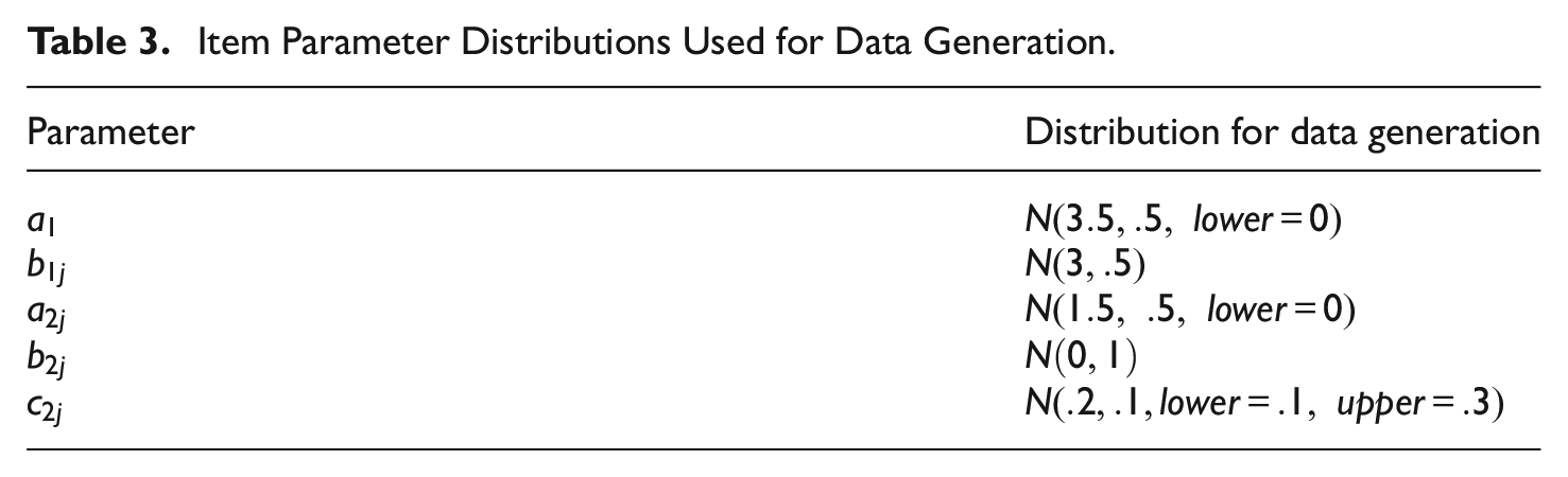
For each replication, we randomly selected item parameters from distributions based on the results of the empirical analysis, as shown in Table 3. We generated a strong invariant relationship between the DISENG trait and each item ( $a_{1}$ ) and high stage 1 item difficulties ( $b_{1 j}$ ). Under the IRTree model, three responses were generated: a rapid response, a non-rapid incorrect response, and a rapid correct response.

Table 3.

Item Parameter Distributions Used for Data Generation.

Parameter	Distribution for data generation
$a_{1}$	$N (3.5, . 5, lower = 0)$
$b_{1 j}$	$N (3, . 5)$
$a_{2 j}$	$N (1.5, . 5, lower = 0)$
$b_{2 j}$	$N (0, 1)$
$c_{2 j}$	$N (. 2, . 1, lower = . 1, upper = . 3)$

Analysis

We fit the IRTree model and the 3-PL model to the simulated data. Because these data were analyzed with the 3-PL, when a response was generated to be rapid, we simulated it to be correct with a 20% chance, representing a random guess on a five-option item. The models were fit to the data using the same Bayesian conditions (e.g., prior distributions, Markov chain iterations) as those presented in Part 1. Because the primary purpose of the simulation study was to consider differences between the two models in the recovery of the TOI trait, recovery of the other model parameters was not pursued. To investigate the bias of the TOI trait, we used posterior means as parameter estimates. Specifically, we calculated bias as the difference between estimated EAP TOI and true TOI.

Results

The pattern of differences in bias in estimating the TOI between the two models depends on true TOI and the number of rapid responses in a response set but does not depend on sample size nor whether there is a high or low RG rate in the sample. In Figure 11, bias is averaged across individuals with the same true TOI (when rounded to the 100th place) across replications, and simulees are grouped by the percentage of rapid responses in a response set using the same categorization as presented in Table 2. Trivial differences exist between bias in TOI under the 3-PL and the IRTree model for individuals with low abilities across conditions, with both resulting in small positive bias regardless of the number of rapid responses. As true TOI increases, the 3-PL results in more biased estimates as compared with the IRTree model as rapid responses in response sets become more prevalent. The IRTree model results in equal or less absolute biased estimates across true TOI for nearly every rapid response categorization level in each of the four conditions. Regardless of whether there is a high or low RG rates in the sample, the IRTree model results in less (absolute) biased TOI estimates for simulees with higher percentages of rapid guesses in their response sets.

Figure 11.

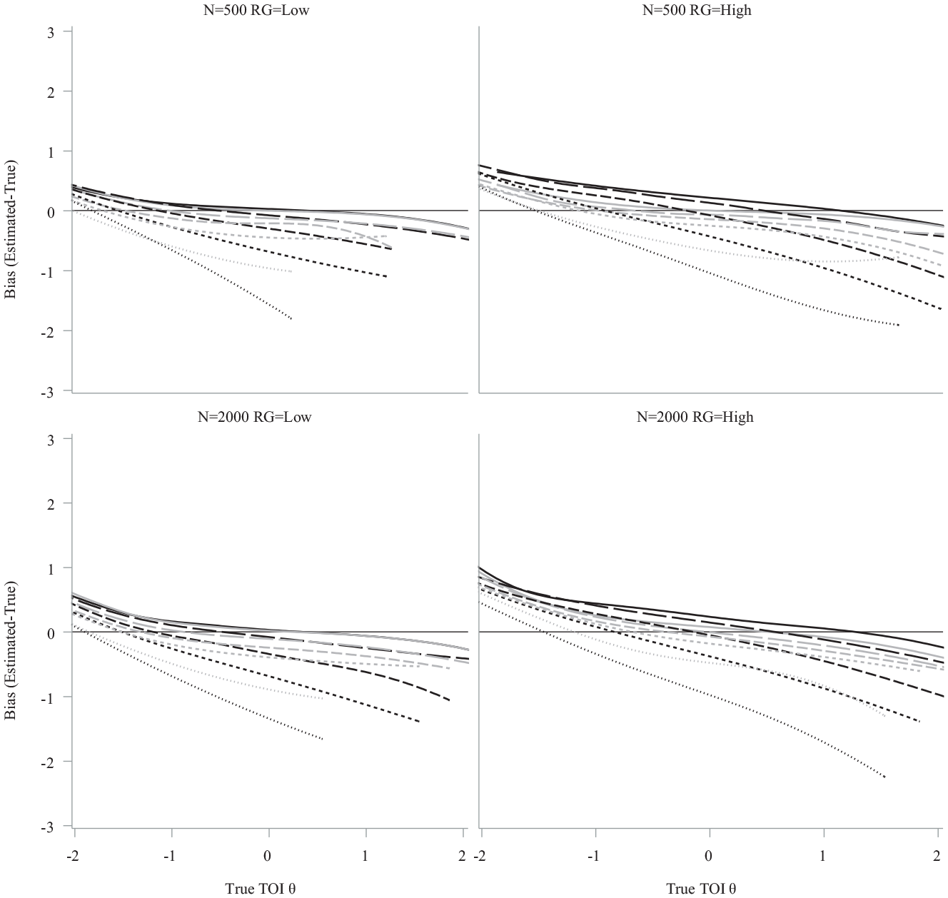
Mean Bias in Trait of Interest by True TOI ( $θ$ ) Across Replications Between the 3-PL (Black) and IRTree Model (Gray) in the Four Simulation Conditions for Groups of Response Sets With Rapid Responses on 0% (Solid), Greater Than 0% but Less Than or Equal to 5% (Long Dash), Greater Than 5% but Less Than or Equal to 10% (Medium Dash), Greater Than 10% but Less Than or Equal to 25% (Dash), Greater Than 25% but Less Than or Equal to 50% (Short Dash), and Greater Than 50% (dot), of the Items.

Discussion

Examinees may espouse differential test-taking behavior and engagement throughout the completion of assessments. Researchers and practitioners must deal with two overarching issues: how to identify disengagement and how to adjust trait estimates for this behavior. Both self-report and process data methods have been used to identify disengagement, with the use of rapid guessing indices being a common and accessible approach. Once rapid guesses are identified, methods ranging from listwise deleting examinees with low effort to modern missing data techniques have been employed to adjust trait scores. In this study, we propose a novel IRTree model to complement these methods, where our method advantageously allows for dependence between rapid guessing behavior and the TOI, analyzes all examinee response sets, adjusts scores for individuals who engage in rapid guessing, and simultaneously models the TOI and a latent disengagement trait.

Although many methods for adjusting scores for low effort assume independence between disengagement and the TOI, prior research has been inconsistent on whether the TOI is related to disengagement. To explain the potential for a relationship, Rios et al. (2017) turned to self-worth theory (e.g., Covington & Beery, 1976). They note that to protect one’s own self-esteem, examinees may exhibit less effort when their expectation of success is low. Therefore, they have an alternative explanation of their poor performance (low effort) rather than receiving evidence of their low ability. This theory was supported by Rios and Soland (2022) who found fear of failure as a moderator of rapid guessing. Regardless of the explanation, the IRTree provides flexibility in that it provides measurement of both the TOI and disengagement at the latent level and allows a relationship between tendencies to rapidly guess and the TOI. Using an application in higher education assessment, we illustrate use of this model and provide validity evidence supporting interpretation of the DISENG trait as disengagement. However, of concern is the necessity to establish a prior distribution for the trait in the Bayesian framework used for estimation. In our study, we assumed a multivariate normal distribution; however, this assumption may not be fully justified. The underlying pattern of rapid guess tendencies is strongly positively skewed. Through estimation, the disengagement trait also relays significant positive skew but results in a bimodal distribution. Due to high item difficulties and high item discrimination in Stage 1 of the model, we can only reliably measure individual differences among examinees with high disengagement. Variation in trait estimates at the lower end of the distribution is a combined result of the selected prior and the estimated relationship with the TOI, which was strong in our example. We encourage further exploration of the assumed prior for alternative distributions.

The purpose of the first study in this paper was to propose the model and illustrate its utility by applying the model along with the 3-PL to real data. It is essential that this model be analyzed using simulation techniques to ascertain its performance under different combinations of sample sizes and levels of disengagement, among other factors. In the second study of this article, we employed a small simulation design to examine the bias of the TOI under varying conditions of sample size and rates of disengagement. By disaggregating results by levels of disengagement in each condition, we determined that bias in TOI estimates was lower when data were fit with the IRTree model as compared with the 3-PL. Moreover, bias depended on the frequency of rapid responding but not the rate of rapid responding in a sample nor sample size.

Due to the limited scope of this simulation, we had to make design choices that limit the generalization. First, we fixed the correlation among the traits to be −.70, a strong relationship as evidenced in our empirical study. Given that this correlation is not always evidenced in empirical studies, a more comprehensive simulation study should investigate varying levels of this correlation. Second, our simulation primarily focused on conditions related to our empirical data study, where we fixed the number of items to 40. Further exploration should investigate varying the number of items and its relationship with sample size. Third, we limited our investigation to bias of the TOI. Future simulation studies can explore the efficacy of the model through model fit indices comparison, item parameter recovery, or further investigation of the TOI by examining its precision. Finally, given the complexity of the model, sample size remains of concern, particularly in real-world applications, where sample size is fixed as in the current study. Because Bayesian estimation is used, parameter estimation depends on the interaction of sample size and prior information. Therefore, further simulation work can help inform minimum appropriate prior distributions and sample sizes needed to ensure accurate estimation for increased complexity (e.g., 2-PL versus 1-PL) at various stages under different conditions.

Although our model presents an item difficulty and discrimination in Stage 1—establishing a relationship between the DISENG trait and the tendency to rapidly guess on an item—we consider our model to be ripe for extension. First, we used an item-invariant discrimination in Stage 1. We made this decision to minimize the number of item parameters given our low sample size. However, the relationship between each item and the DISENG trait could be explored through item-specific Stage 1 discrimination estimates. Second, a longitudinal extension can be used to investigate effort fluctuations throughout an exam. Given that motivation changes throughout an exam (e.g., Pastor et al., 2019) researchers can allow the disengagement trait to vary longitudinally, by treating items or groups of items (e.g., sections of the test) as time points. Furthermore, if interventions to increase motivation are imposed throughout an exam, like those as a consequence of rapid guessing in Wise et al. (2006) or those at fixed time intervals in Ong et al. (2018), researchers can investigate their effects on disengagement trait estimates if allowed to vary longitudinally. Longitudinal extensions of IRTree models already exist in the noncognitive literature (e.g., Ames & Leventhal, 2022) and can therefore be translated to more cognitive assessments as needed. Furthermore, IRTree models lend themselves to covariate extensions, whether item or person parameter predictors (Jeon & De Boeck, 2016). These extensions can assist answering important questions, such as what item characteristics (e.g., word length, mediated items; Rios & Soland, 2022; Wise et al., 2021) can predict rapid guessing as well as what person characteristics (e.g., SES, linguistic background; Rios & Soland, 2022) lead to higher tendencies of RG behavior. Finally, in our illustration we used the 3-PL model in Stage 2. Strategic selection of the IRT model in Stage 2 (or an extension to more than two stages) allows adapting the model to a variety of item types, such as cognitive items requiring sequential steps through the use of sequential IRT models (e.g., Tutz, 2016), or to non-cognitive items through the use of the graded response model (Samejima, 1969).

IRTree models have recently garnered significant research attention in the self-report survey literature (e.g., Tijmstra et al., 2018). There have been many studies implementing IRTree models in applied settings (e.g., Ames & Leventhal, 2023; Spratto et al., 2021) and Plieninger (2021) wrote an extensive piece outlining their accessibility to practitioners. This suggests that although they are multidimensional IRT (MIRT) models, their use is more widespread than some other complex MIRT models. However, there have been limited examples of IRTree models applied to cognitive assessments (e.g., Myers et al., 2020) even though they are prevalent in the noncognitive literature. In limited examples, they have been applied to answer-change and non-response behavior (Jeon et al., 2017).

In our simple, accessible two-stage IRTree model, we disaggregate respondent behavior into a disengagement indicator and an accuracy indicator. We combine the IRTree response process approach with using response time thresholds as indicators of rapid guessing behavior. We exemplify this model using a response time threshold cut-point of 10% of the mean item response time, but this model can easily accommodate other procedures for establishing thresholds. This is because the threshold indicator of item-level disengagement is determined prior to applying the model.

Overall, the IRTree provides an accessible approach to adjust latent ability for RG behavior as well as providing a useful framework for answering future research questions about examinee engagement. We demonstrate the efficacy of the model trait estimates capturing rapid guessing behavior using total response time and scores on a self-report effort scale as criterion. Moreover, we show how the IRTree model reduces the uncertainty in trait estimates, especially prevalent when respondents rapidly guess on at least one item. We also examined response profiles for students to understand how disengagement leads to adjustments of the latent abilities with the IRTree as compared to the traditional 3-PL model. Finally, we showed that in a limited simulation, the IRTree model results in less biased TOI estimates when individuals rapidly respond to a high number of items in a response set. We hope this model is of use to both practitioners and researchers exploring the use of RG to investigate effort and engagement.

Footnotes

Acknowledgements

We would like to thank Paulius Satkus for his contributions to this research.

Declaration of Conflicting Interests

The authors declared no potential conflicts of interest with respect to the research, authorship, and/or publication of this article.

Funding

The authors received no financial support for the research, authorship, and/or publication of this article.

ORCID iDs

Brian Leventhal

Dena Pastor

Notes

References

American Educational Research Association, American Psychological Association, National Council on Measurement in Education, Joint Committee on Standards for Educational & Psychological Testing. (2014). Standards for educational and psychological testing.

Ames

A. J.

Leventhal

B. C.

(2022). Modeling changes in response style with longitudinal IRTree models. Multivariate Behavioral Research, 57(5), 859–878. https://doi.org/10.1080/00273171.2021.1920361

Ames

A. J.

Leventhal

B. C.

(2023). Application of a longitudinal IRTree model: Response style changes over time. Assessment, 30(2), 332–347. https://doi.org/10.1177/10731911211042932

Covington

M. V.

Beery

(1976). Self-worth and school learning. Holt, Rinehart & Winston.

Debeer

Janssen

Boeck

P. D.

(2017). Modeling skipped and not-reached items using IRTrees. Journal of Educational Measurement, 54(3), 333–363. https://doi.org/10.1111/jedm.12147

De Boeck

Partchev

(2012). IRTrees: Tree-based item response models of the GLMM family. Journal of Statistical Software, 48(1), 1–28. https://doi.org/10.18637/jss.v048.c01

Deribo

Kroehne

Goldhammer

(2021). Model-based treatment of rapid guessing. Journal of Educational Measurement, 58(2), 281–303. https://doi.org/10.1111/jedm.12290

Jeon

De Boeck

(2016). A generalized item response tree model for psychological assessments. Behavior Research Methods, 48(3), 1070–1085. https://doi.org/10.3758/s13428-015-0631-y

Jeon

De Boeck

van der Linden

(2017). Modeling answer change behavior: An application of a Generalized Item Response Tree Model. Journal of Educational and Behavioral Statistics, 42(4), 467–490. https://doi.org/10.3102/1076998616688015

10.

Kong

X. J.

Wise

S. L.

Bhola

D. S.

(2007). Setting the response time threshold parameter to differentiate solution behavior from rapid-guessing behavior. Educational and Psychological Measurement, 67(4), 606–619. https://doi.org/10.1177/0013164406294779

11.

Liu

Luo

(2019). Modeling test-taking non-effort in MIRT models. Frontiers in Psychology, 10, 1–12. https://doi.org/10.3389/fpsyg.2019.00145

12.

Myers

A. J.

Ames

A. J.

Leventhal

B. C.

Holzman

M. A.

(2020). Validating rubric scoring processes: An application of an item response tree model. Applied Measurement in Education, 33(4), 293–308. https://doi.org/10.1080/08957347.2020.1789143

13.

Ong

T. Q.

Pastor

D. A.

Yang

S.-T.

(2018). The effects of administering alerts at fixed points during a low-stakes test [Paper presentation]. Annual meeting of the American Educational Research Association, New York, NY, United States.

14.

Pastor

D. A.

Ong

T. Q.

Strickman

S. N.

(2019). Patterns of solution behavior across items in low-stakes assessments. Educational Assessment, 24(3), 189–212. https://doi.org/10.1080/10627197.2019.1615373

15.

Plieninger

(2021). Developing and applying IR-Tree Models: Guidelines, caveats, and an extension to multiple groups. Organizational Research Methods, 24(3), 654–670. https://doi.org/10.1177/1094428120911096

16.

Rios

J. A.

Deng

(2021). Does the choice of response time threshold procedure substantially affect inferences concerning the identification and exclusion of rapid guessing responses? A meta-analysis. Large-Scale Assessments in Education, 9(1), Article 18. https://doi.org/10.1186/s40536-021-00110-8

17.

Rios

J. A.

Guo

Mao

Liu

O. L.

(2017). Evaluating the impact of careless responding on aggregated-scores: To filter unmotivated examinees or not? International Journal of Testing, 17(1), 74–104. https://doi.org/10.1080/15305058.2016.1231193

18.

Rios

J. A.

Soland

(2022). An investigation of item, examinee, and country correlates of rapid guessing in PISA. International Journal of Testing, 22(2), 154–184. https://doi.org/10.1080/15305058.2022.2036161

19.

Samejima

(1969). Estimation of latent ability using a response pattern of graded scores. Psychometrika Monograph Supplement, 34(4, Pt. 2), 100.

20.

SAS Institute Inc. (2018). SAS/STAT® 15.1 user’s guide.

21.

Spratto

E. M.

Leventhal

B. C.

Bandalos

D. L.

(2021). Seeing the forest and the trees: Comparison of two IRTree models to investigate the impact of full versus endpoint-only response option labeling. Educational and Psychological Measurement, 81(1), 39–60. https://doi.org/10.1177/0013164420918655

22.

Sundre

D. L.

Wise

S. L.

(2003). “Motivation filtering”: An exploration of the impact of low examinee motivation on the psychometric quality of tests[Paper presentation]. Annual meeting of the National Council on Measurement in Education, Chicago, IL, United States.

23.

Thelk

A. D.

Sundre

D. L.

Horst

S. J.

Finney

S. J.

(2009). Motivation matters: Using the student opinion scale to make valid inferences about student performance. The Journal of General Education, 58(3), 129–151. https://doi.org/10.1353/jge.0.0047

24.

Tijmstra

Bolsinova

Jeon

(2018). General mixture item response models with different item response structures: Exposition with an application to Likert scales. Behavior Research Methods, 50(6), 2325–2344. https://doi.org/10.3758/s13428-017-0997-0

25.

Tutz

(2016). Sequential models for ordered responses. In van der Linden

W. J.

Hambleton

R. K.

(Eds.), Handbook of item response theory (Vol. 1, pp. 167–180). Springer.

26.

Wise

S. L.

(2006). An investigation of the differential effort received by items on a low-stakes computer-based test. Applied Measurement in Education, 19(2), 95–114. https://doi.org/10.1207/s15324818ame1902_2

27.

Wise

S. L.

(2015). Effort analysis: Individual score validation of achievement test data. Applied Measurement in Education, 28(3), 237–252. https://doi.org/10.1080/08957347.2015.1042155

28.

Wise

S. L.

Bhola

D. S.

Yang

(2006). Taking the time to improve the validity of low stakes tests: The effort monitoring CBT. Educational Measurement: Issues and Practice, 25(2), 21–30. https://doi.org/10.1111/j.1745-3992.2006.00054.x

29.

Wise

S. L.

DeMars

C. E.

(2005). Low examinee effort in low-stakes assessment: Problems and potential solutions. Educational Assessment, 10(1), 1–17. https://doi.org/10.1207/s15326977ea1001_1

30.

Wise

S. L.

DeMars

C. E.

(2006). An application of item response time: The Effort-Moderated IRT model. Journal of Educational Measurement, 43(1), 19–38. https://doi.org/10.1111/j.1745-3984.2006.00002.x

31.

Wise

S. L.

Kong

(2005). Response time effort: A new measure of examinee motivation in computer-based tests. Applied Measurement in Education, 18(2), 163–183. https://doi.org/10.1207/s15324818ame1802_2

32.

Wise

S. L.

Pastor

D. A.

Kong

X. J.

(2009). Correlates of rapid-guessing behavior in low-stakes testing: Implications for test development and measurement practice. Applied Measurement in Education, 22(2), 185–205. https://doi.org/10.1080/08957340902754650

33.

Wise

S. L.

Smith

L. F.

(2011). A model of examinee test-taking effort. In Bovaird

J. A.

Geisinger

K. F.

Buckendahl

C. W.

(Eds.), High-stakes testing in education: Science and practice in K–12 settings (pp. 139–153). American Psychological Association.

34.

Wise

S. L.

Soland

Dupray

L. M.

(2021). The impact of technology-enhanced items on test-taker disengagement. Journal of Applied Testing Technology, 22(1), 28–36.