Evaluating Change in Adjusted R -Square and R -Square Indices: A Latent Variable Method Application

Abstract

A procedure for interval estimation of the difference in the adjusted R-square index for nested linear models is discussed. The method yields as a byproduct confidence intervals for their standard R-square difference, as well as for the adjusted and standard R-squares associated with each model. The resulting interval estimate of the difference in adjusted R-square represents a useful and informative complement to the commonly used R-square change statistic and its significance test in model selection and contains substantially more information than that test. The outlined procedure is readily employed with popular software in empirical educational and psychological studies and is illustrated with numerical data.

Keywords

nested models

Linear modeling is one of the most frequently employed analytic approaches in the educational and psychological sciences (e.g., Agresti, 2018). Its applications in these and cognate disciplines frequently involve more than one model for a given outcome and set of explanatory variables (predictors, covariates, independent variables; e.g., Harrell, 2015). An issue of central importance then is that of model comparison, when for a response measure of interest one may consider two or more successively inclusive groups of predictors (e.g., Judd et al., 2017). This concern oftentimes arises in model selection in the utilization of regression analysis in empirical studies, which can be viewed as a process of seeking an optimal subset of an initial set of predictors according to pre-specified criteria (e.g., Draper & Smith, 1998).

Contemporary applications of regression modeling for variable selection purposes in behavioral and social research almost routinely employ the change in the R-square index for models of concern and occasionally involve the adjusted R-square statistic for comparing their fit to analyzed data (e.g., Field, 2018). Evaluation of the relative increment or loss in the standard or conventional (regular) R-square index for nested models with the same response variable, for example pairs of models where one involves the predictors in the other plus additional ones, is facilitated then by the widely available change in R-square statistic and its often-used test of significance (cf. Agresti, 2018). This test merely evaluates, however, the strength of data evidence against the null hypothesis of no change in the R-square due to the addition or deletion of predictors, rather than the possible magnitude of the associated population increase or decrease in model explanatory power. For this reason, the result of the frequently utilized R-square change test contains rather limited information (cf. Schmidt, 1996). In addition, the (standard) R-square index is itself known to be an “optimistic” estimate of model fit in a studied population, due to the underlying model fitting process being based on the minimization of the least squares discrepancy function (e.g., Casella & Berger, 2002).

To counteract this positive bias of the standard R-square index, the adjusted R-square has been introduced as a model fit measure that is less biased and more informative about a model’s explanatory power at large (e.g., Harrell, 2015). Yet, no widely available procedure seems to exist that could be readily used by the general educational or psychological scholar to obtain a confidence interval (CI) of the difference in the adjusted R-square indices, or in the standard R-square indices, for two nested models. These interval estimates provide substantially more information than hypothesis tests, in particular about the plausible magnitude of the model difference in R-squares or adjusted R-squares in a population under investigation (Agresti, 2018).

The purpose of this note is to contribute to filling this gap by discussing a method for interval estimation of the change in each of these R-square indices for two nested models. The procedure can be developed within the comprehensive latent variable modeling (LVM) methodology framework (B. O. Muthén, 2002), thus facilitating its possible extension subsequently to more general models with latent variables, and is straightforwardly employed with popular software. The approach renders as a byproduct also an easily utilized means for testing hypotheses, if indeed needed, about pre-specified values for the model difference in the adjusted or standard R-square (including that of no change in any of these indices, in case of real concern per se), and is illustrated with numerical data.

Background, Notation, and Assumptions

In the remainder of this note, we assume that a response (outcome, dependent) variable y and a set of possible explanatory variables x₁, x₂, …, x_k are of research interest (k > 1; e.g., Agresti, 2018). In applications of regression analysis in the behavioral and social sciences, two or more subsets of these predictors can be under consideration, which gives rise to competing models explaining variance in the outcome measure (e.g., Draper & Smith, 1998). We presume that y is a continuous observed variable (or can be treated as continuous for certain purposes of relevance), while the predictors are assumed to be perfectly measured and with positive variance (e.g., Bollen, 1989). We stipulate that all p = k + 1 variables are given and thus the only ones of concern, and assume that they have been administered to a sample of units of analysis from a studied population that is not associated with clustering effects or substantial unobserved heterogeneity (e.g., Geiser, 2013; Rabe-Hesketh & Skrondal, 2022; see “Discussion and Conclusion” section for possible assumption relaxation).

In this empirically relevant setting with wide applicability across the educational and behavioral disciplines, suppose a researcher is considering two nested models for the response variable y, with one of them having all k predictors while the other involving only r of them (0 < r < k). Designating the former model as M1 and the latter as M2, we assume without loss of generality that the predictors in M2 are the first r variables x₁, x₂, …, x_r. We stress that both models have the same response variable, with the explanatory variable set of the “reduced” model M2 being a proper subset of that of the “full” model M1 (Judd et al., 2017).

As indicated earlier, the following discussion is concerned with model comparison (model choice), that is, with means allowing a researcher to select, based on empirical evidence, one of the models as preferable to the other. In other words, suppose that a scholar is interested in selecting either M1 as preferable to M2, or M2 as preferable to M1. When two such models differ by only one predictor, the model choice is facilitated by testing for the significance of this predictor in the full model (e.g., Agresti, 2018; see also below). The rest of the article deals predominantly with a more general case of model selection, where at least two predictors in one of the models are not included in the other. However, all developments in the sequel are directly applicable also when the two models differ by just one predictor. This includes in particular the use of the following interval estimates for the change in adjusted R-square and in standard R-square when removing the predictor in question. These estimates contain, as indicated, markedly more information about the population model differences in any of these indices than the predictor significance test. In particular, they contain more information than the test of no associated change in the standard R-square, which is nearly routinely utilized at present by empirical scholars (Draper & Smith, 1998). For this reason, the intervals could be recommended for use more broadly and possibly as replacements in general for the latter test (Draper & Smith, 1998; see also “Discussion and Conclusion” section).

The remaining discussion may be considered evolving within the comprehensive framework of the general LISREL model (e.g., Jöreskog & Sörbom, 1996), which is defined by the following two equations (assuming I_q − B as invertible, with I_q denoting the identity matrix of size q; q ≥ 1):

y = μ + Λ η + ε,

(1)

η = B η + δ .

(2)

In Equations (1) and (2), the p × 1 vector y consists of the above p observed variables (the response variable and the k predictors), µ is the p × 1 vector of their respective means, Λ is the p × q factor loading matrix, η is the q × 1 vector of factors assumed with zero means, B is the q × q matrix of structural relationships, and ε and δ are the residual term vectors correspondingly of size p × 1 and q × 1, with the usual assumptions of uncorrelated residuals among themselves and with the factors (see also Bollen, 1989).

The standard regression model (e.g., Draper & Smith, 1998) is a special case of the general LISREL model, as is widely appreciated when all observed variables are considered set equal to respective dummy variables ζ₁, ζ₂, …, ζ_k + 1 that are associated each with zero error term, Λ is the p × p identity matrix, η is the p × 1 vector of those dummy variables, and p = k + 1 (e.g., Raykov, 2001, and references therein). The consideration of the general LISREL model as an inclusive framework for the following developments relates the latter to latent variable methods (cf. Marcoulides & Raykov, 2019), and provides a possibility for extending in future research the discussion in this note to adjusted R-square indices and their evaluation for more general models containing proper latent variables (Bollen, 1989; see also “Discussion and Conclusion” section).

Point and Interval Estimation of the Change in the Adjusted R-Square and the Standard R-Square Indices

In the above notation, the multiple linear regression model that underlies this note is as follows:

y = b_{0} + b_{1} x_{1} + b_{2} x_{2} + \dots + b_{k} x_{k} + ε,

(3)

which was earlier referred to as the full model and denoted M1 (e.g., Draper & Smith, 1998). The reduced model M2 is nested in M1 and utilizes only r of its explanatory variables (0 < r < k), that is, M2 is defined as:

y = b_{0} + b_{1} x_{1} + b_{2} x_{2} + \dots + b_{r} x_{r} + ε

(4)

where for convenience we use the same notation for intercept, partial regression coefficients, and model error term (Judd et al., 2017).

Denoting the standard R-square index as R², the adjusted R-square index R²_a is defined in model M1 and any model nested in it as:

{R^{2}}_{a} = 1 - \frac{(1 - R^{2}) (n - 1)}{(n - s - 1)},

(5)

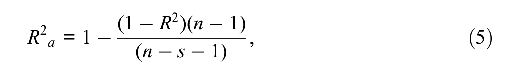
where s denotes the number of its explanatory variables (1 ≤ s ≤ k) and n sample size. Alternatively, R²_a can be equivalently defined as:

{R^{2}}_{a} = R^{2} - \frac{s (1 - R^{2})}{(n - s - 1)}

(6)

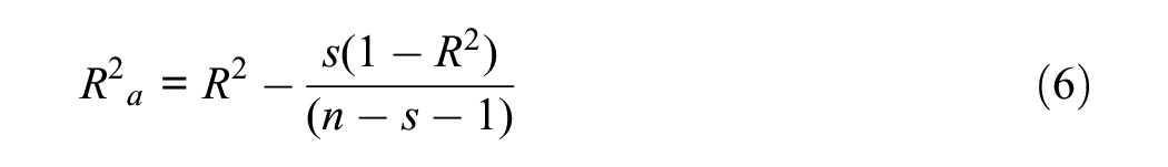
(Agresti, 2018). The right-hand side of Equation (6) shows that the downward correction of R² that is achieved by R²_a, which is denoted C, is:

C = \frac{s (1 - R^{2})}{(n - s - 1)} .

(7)

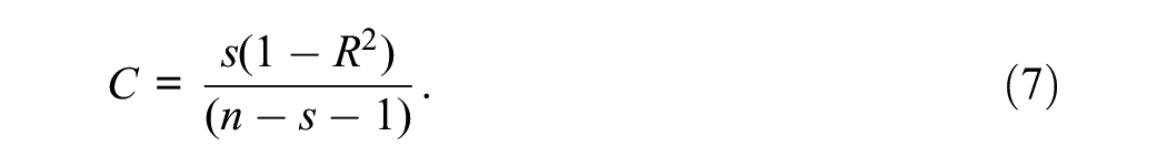
From Equation (7), it is seen that this correction C increases when (a) sample size decreases, (b) the number of predictors increases, or (c) R² itself decreases, all else kept correspondingly constant. Hence, when the sample size is small, the number of predictors is large, or R² is limited, the discrepancy between R² and its adjusted version is relatively large. This corresponds to the observation that in (a), (b), or (c) (or any combination of these circumstances) the positive bias of R² grows (cf. Draper & Smith, 1998). In addition, Equation (6) highlights the fact that the adjusted R-square index can decrease when one or more explanatory variables are added to a given set of predictors, unlike the standard R-square that cannot decrease when adding a predictor.¹

Based on Equations (6) and (7), the difference in the adjusted R-squares, denoted ΔR²_a, for two nested models differing in t predictors (t ≥ 1) is:

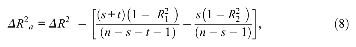
Δ {R^{2}}_{a} = Δ R^{2} - [\frac{(s + t) (1 - R_{1}^{2})}{(n - s - t - 1)} - \frac{s (1 - R_{2}^{2})}{(n - s - 1)}],

(8)

where ΔR² = R₁² − R₂² is the difference in the standard R-squares (with R₁² pertaining to the model with more predictors, and similarly for its adjusted version; 1 ≤ s + t ≤ k).

Equation (8) shows the change in adjusted R-square across two nested models as a function of the associated change in standard R-square, sample size, and the number of predictors in the models. Since the R-square index is itself a function of the model parameters, in formal notation therefore the following relationship holds:

Δ {R^{2}}_{a} = Δ {R^{2}}_{a} (n, s_{1}, s_{2}, θ_{1}, θ_{2}),

(9)

where s₁ and s₂ are the numbers of predictors in models M1 and M2, with respective parameter vectors θ₁ and θ₂ (consisting of the pertinent intercept, partial regression coefficients, and residual variance; 1 ≤ s₁ ≠ s₂ ≤ k). Equation (9) also demonstrates that the adjusted R-square difference is such a function of sample size, number of model parameters, and these parameters, which is continuously differentiable in each parameter (e.g., Apostol, 2006).

Based on Equation (9), once the full and reduced models M1 and M2 are fit to a given data set, point and interval estimation of their difference in adjusted R-square and standard R-square becomes possible. More specifically, the point estimate of the latter difference statistic is obtained by direct subtraction of the individual R-square estimates (capitalizing on relevant features of used software, with the standard R-square difference and individual adjusted R-squares being routinely provided by canned software; see next). In fact, revisiting Equations (3) and (4) one realizes that for either model the standard R-square is the complement to 1 of the residual variance in its standardized solution (since the variance of y is set at 1 in that solution; this variance estimate is automatically provided for instance by the LVM software Mplus employed later in the note), and thus ΔR² = R₁² − R₂² can be point estimated by the difference of the residual variance estimates in the standardized solutions for M1 and M2; (B. O. Muthén et al., 2016). From this estimate of ΔR², that of the difference in adjusted R-squares is furnished readily by Equation (8), in addition to the adjusted R-square estimates of the two models (see Equation (5) or (6) for them and Appendix 2 for pertinent software utilization).

Next, we make use of the above-indicated continuous differentiability of the adjusted R-square difference in Equation (9), for interval estimation of the indices of main interest in this article. In particular, CIs of the differences in adjusted R-squares and standard R-squares, as well as for the individual model adjusted and standard R-square indices, can be furnished at any pre-specified confidence level with the bootstrap approach (using say g = 2,000 resamples with replacement from the original data set; Efron & Tibshiriani, 1993). Specifically, bootstrap CIs can be obtained for the difference in adjusted R-squares and in standard R-squares, as well as for the individual model adjusted and standard R-squares, by taking as their lower and upper endpoints the relevant quantiles of the bootstrap distributions of their corresponding estimates (e.g., the 2.5th and 97.5th quantiles for a 95% CI). This bootstrap application can be readily conducted using the widely used packages Mplus and Stata (see next section for a demonstration).

We emphasize that the resulting CI for the difference in standard R-squares when comparing models M1 and M2 contains substantially more information than the currently almost routinely employed test for the significance of the change in standard R-square (the “multiple F-test”) in educational and psychological research (cf. Judd et al., 2017). The reason is that as pointed out earlier this test and its p-value only indicate the strength of empirical evidence against the hypothesis of no difference in the R-squares for both models. Yet, a CI for this difference provides markedly more information since the CI shows how large the magnitude of this R-square difference can plausibly be in a population of concern. No less important, as shown above, the outlined interval estimation procedure furnishes also a CI for the difference in adjusted R-squares for two nested models. This CI seems not to have been used in current or previously conducted empirical behavioral and social studies, but we submit that it is at least as relevant for such models. The reason is that due to the more pronounced positive bias in the standard R-square, the CI for the adjusted R-square difference is in fact a CI for a better-evaluated difference in population explanatory power of the models in question (see “Introduction” section and earlier discussion; cf. Agresti, 2018). This CI for the difference in adjusted R-squares for nested models is now readily available with the approach described in the present note and extends significantly the arsenal of means for studying linear models that is available to behavioral and social scholars.

The outlined point and interval estimation procedure for the difference in the adjusted and standard R-square indices is demonstrated on data next.

Illustration on Data

For our method demonstration purposes in this section, we use a simulated data set for a response variable, y, and k = 20 predictors, x₁, …, x₂₀. The data set was generated for n = 50 cases according to the following model:

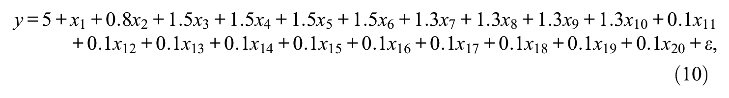
\begin{matrix} y = 5 + x_{1} + 0.8 x_{2} + 1.5 x_{3} + 1.5 x_{4} + 1.5 x_{5} + 1.5 x_{6} + 1.3 x_{7} + 1.3 x_{8} + 1.3 x_{9} + 1.3 x_{10} + 0.1 x_{11} \\ + 0.1 x_{12} + 0.1 x_{13} + 0.1 x_{14} + 0.1 x_{15} + 0.1 x_{16} + 0.1 x_{17} + 0.1 x_{18} + 0.1 x_{19} + 0.1 x_{20} + ε, \end{matrix}

(10)

where ε was simulated as a zero-mean normal variate with a variance of 50 and independent of the predictors, all predictors were normal with zero means, x₁ and x₂ had a variance of 2, x₃ through x₆ variance of 1.5, x₇ through x₁₀ variance of 1.3, and the remaining predictors had each a variance of 0.1. (The data simulation process was carried out with the first Mplus command file in Appendix 1, referred to as Code 1; using it with its seed will generate the same data set when interested in replicating the results reported next).

In the rest of this section, in line with the discussion in the last we are interested in comparing (a) the above full model with all predictors, M1 (see Equation (10)), to (b) the reduced model M2 with the first 10 predictors only. Accordingly, to enable this model comparison, we generate first g = 2,000 resamples with replacement from the simulated data set (see the second Mplus command file in Appendix 1, referred to as Code 2). Then we fit models M1 and M2 to each of these 2,000 resamples, requesting their standardized solutions and saving the individual model parameter estimates (see the third Mplus command file in Appendix 1, referred to as Code 3). On the set of results from both models, we estimate next with Stata (see Appendix 2), (i) their standard R-squares (as the complements to 1 of their standardized solution residual variances—see preceding section and the Notes to Code 3 in Appendix 1); (ii) their adjusted R-squares using Equation (5); (iii) the differences in the adjusted R-squares and the standard R-squares across M1 and M2; and in (iv) the 2.5th and 97.5th quantiles of the bootstrap distributions of the adjusted and standard R-squares, as well as of their respective differences in across models. These quantiles represent then correspondingly the lower and upper limit of the 95% CIs of these four parameters of main interest in this article and are displayed together with related estimates in Table 1.

Table 1.

Bootstrap 95% CIs and Means Across Resamples for Standard and Adjusted R-squares As Well As Their Differences.

Parameter	Model
	M1		M2		D
	A	95% CI	A	95% CI	A	95% CI
R ²	0.750	[0.571, 0.915]	0.517	[0.346, 0.692]
R ² _a	0.577	[0.275, 0.856]	0.394	[0.172, 0.615]
ΔR²					0.232	[0.084, 0.422]
ΔR²_a					0.183	[−0.050, 0.470]

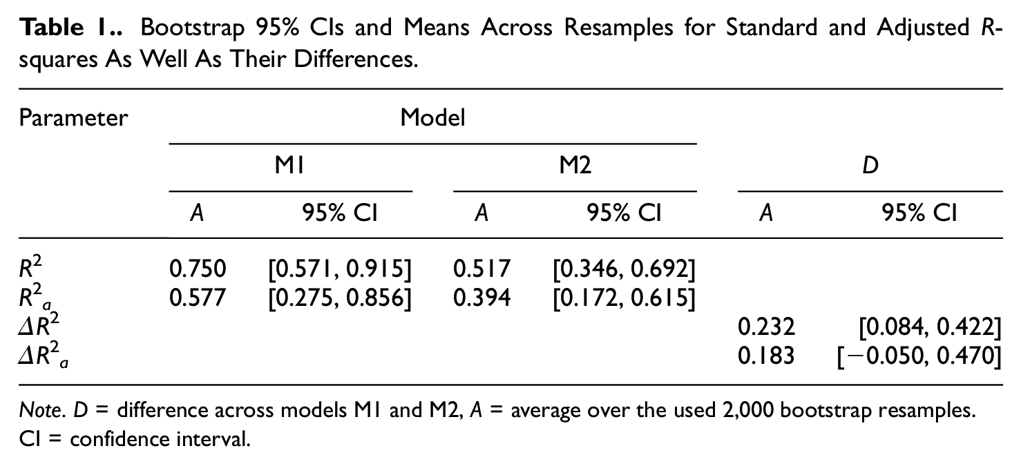
Note. D = difference across models M1 and M2, A = average over the used 2,000 bootstrap resamples. CI = confidence interval.

As seen from Table 1, the 95% CI for the model difference in the standard R-square index across the full and restricted models is [0.084, 0.422], and is thus entirely positioned above 0. This can be interpreted as suggesting (if using only this index and its difference) the need for keeping in M1 the last 10 predictors x₁₁ through x₂₀ in addition to the first 10 included in both models, x₁ through x₁₀. Hence, if using the standard R-square index, one would prefer the less parsimonious model M1 with all 20 predictors (see also below). However, as found also in Table 1, the CI for the difference in their adjusted R-square index is [−0.050, 0.470] and contains 0. The last finding is interpreted as suggesting that (i) the equality in the adjusted R-squares for M1 and M2 is highly plausible in the population, and hence (ii) the last 10 predictors, x₁₁ through x₁₀, can be removed. This implies preferring M2 to M1, that is, the more parsimonious model M2 with the first 10 predictors only, rather than preferring M1 contains all 20 predictors as suggested by the standard R-square change and its CI.

Since we know in this section all population or true parameters involved in the data simulation process, we can determine for either model the population proportion of model-explained variance in the response variable y (see Equation (10) and their immediately following discussion; we note in passing that this proportion may be treated as the population or true R-square index that is typically unknown in empirical research). Indeed, with the known partial regression coefficients and predictor variances (see above in this section), one readily works out this ratio of model explained to observed variance in y. Specifically, the population proportion explained variance by model M1 results then as 0.3384318, while for M2 this proportion is obtained as 0.3383443, that is, by less than 0.00009 lower than that proportion for M1. Therefore, keeping the last 10 predictors in the model with all 20 predictors, that is, preferring model M1 as suggested by the standard R-square index, entails a gain of less than 0.0001, which is less than 0.01%, in the population model explanatory power. This gain can be viewed, however, as ignorable for essentially all practical purposes. Therefore, one may well prefer model M2 in the population that has twice as few predictors as M1, a decision also suggested by the adjusted R-square index (see also below). The last conclusion can be seen as a correct decision due to (i) the essentially/practically non-existent population gain, relative to M2, in explanatory power by keeping the last 10 predictors in model M1 in addition to the first 10 of them; and (ii) model M2 being the markedly more parsimonious model, with twice fewer predictors (parameters) than M1. Hence, the present is an example where the widely used difference in standard R-square indices suggests an incorrect conclusion (even if using its CI to reach or corroborate it), while employing instead the difference in adjusted R-squares and associated CI suggests the correct decision.

In addition, the example illustrates a case of what may be characterized as a severe overestimation of the population model explanatory power (population R-square) by the standard R-square index. This positive bias is observed when examining the means (averages) over the 2,000 resamples of the pertinent parameter estimates. More specifically, as seen from Table 1, the mean (average) of these estimates for the standard R-square in model M1 is .750 and thus more than twice larger than its population R-square index (see above). This average is in fact higher than the population R-square by an amount that substantially exceeds that population index. Furthermore, the mean difference in standard R-squares across M1 and M2 is found in that table to be .232. Hence, this mean difference is markedly overestimating the population difference in R-squares (being less than .0001 as found above), and the magnitude of this difference is some 70% of either model’s population R-square (which is found above to be .338, rounded-off). Table 1 also shows a notable, yet considerably less pronounced, overestimation degree of the population explanatory power for either model by the adjusted R-squares. Indeed, this positive bias for M1, with a mean adjusted R-square of .577, is about two-thirds of the population/true R-square for M1 (or M2). In addition, the mean adjusted R-square bias is about four times lower for M2 (relative to M1), with this model M2 being the preferred one as concluded earlier. However, for either model, as observed from Table 1, the mean positive bias of the adjusted R-square is about half of the mean positive bias in the standard R-square index. Relatedly, the mean difference in adjusted R-squares for M1 and M2, being .183, is over 20% smaller than that difference in the standard R-squares (being .232). This discrepancy in the standard and adjusted R-square differences across M1 and M2 is a reason for the opposite conclusions that have been earlier suggested based on the CI of the difference in standard R-squares, relative to that based on the CI of the difference in adjusted R-squares.

We conclude this section by emphasizing that its goal was merely to demonstrate (a) how discrepant conclusions using the difference in adjusted R-squares can be relative to those using the difference in standard R-squares and (b) the different degrees of possible over-estimation of population model explanatory power by the standard R-square and by the adjusted R-square; as well as (iii) the fact that the positive bias in the adjusted R-square index is markedly smaller than that bias in the standard R-square index. A main reason for this discrepancy is the combination of relatively limited sample size, large number of predictors (particularly in M1), and low standard R-square of either model. At the same time, this section did not intend to imply that similar (or larger) discrepancies are to be routinely found in empirical educational and psychological research, while they can be expected to be less likely with higher sample size, lower number of predictors, and higher R-square indices.

Discussion and Conclusion

This note was concerned with the comparison of nested linear models that are widely used in educational and psychological research, and intended to contribute to promoting the use of improved methods and CIs facilitating it. A readily applicable procedure was outlined for point and interval estimation of the adjusted and standard R-square indices for any regression model, and particularly for interval estimation of the difference in adjusted and in standard R-squares for nested models. The approach is readily conducted with popular software, and at least some of the resulting CIs seem to have not been used in empirical behavioral research. Furthermore, the outlined method de-emphasizes testing the frequently examined in applied work hypothesis of no change in the (standard) R-square indices for nested models. This is achieved by shifting much of the attention that the nearly routinely used difference in standard R-squares receives at present, toward CIs for the difference in adjusted R-squares that are each better estimates of model explanatory power (and CIs of the difference in standard R-squares). Moreover, the outlined approach is directly applicable when the two models differ by only one predictor, without any necessary modification. In this way, the approach provides an additional means for gaining further and important information about the population unique predictive power of a single predictor under consideration, which information goes beyond the result of the currently almost routinely employed significance test for dropping a predictor in a regression model (predictor significance test and pertinent p-value; cf. Agresti, 2018).

The procedure discussed in this article is associated with several caveats that need to be attended to when it is applied in empirical research. One of them is the need for the full model to be plausible. Various methods are available in the literature that enable educational and behavioral scholars to examine model plausibility, including in particular regression diagnostics (e.g., Draper & Smith, 1998). Furthermore, we assumed at the outset that the response variable was (approximately) continuous, or treatable as such in certain settings of concern. It may be conjectured that the outlined method may be used in a largely trustworthy way with discrete outcome measures having at least 5 to 7 values and distributions with limited asymmetry (cf. Rhemtulla et al., 2012). However, this conjecture needs to be examined in future research before being recommended, possibly based on extensive simulation studies that are beyond the confines and aims of this article. Also, as stated earlier, our discussion presumed no clustering effects and no substantial unobserved heterogeneity. The latter assumption can be relaxed, leading to mixture regression analysis (e.g., Geiser, 2013), and ensuing within-class model comparison via an application of the discussed procedure. In addition, clustering effects can be accounted for with the used software (L. K. Muthén & Muthén, 2025), enabling thus utilization of the method of this discussion in hierarchical data settings as well. Moreover, the general linear modeling framework, within which the developments in this article have proceeded, seems to allow subsequent extensions of its results to models involving predictors measured with error and at least two indicators of their underlying true values (latent variables; cf. Bollen, 1989). The detailed discussion of all these relaxations, however, lies beyond the frame of this article, and we encourage their explication in future research.

As alluded to earlier, this note did not imply and should not be interpreted as suggesting that the discrepancy between the standard and adjusted R-square indices can always or frequently be expected to be large in empirical studies. In particular, Equations (6) and (7) and their subsequent discussion entail that this difference is more pronounced with smaller samples and smaller R-squares and/or more predictors, as well as with combinations of two or all three of these circumstances (see also earlier discussion). Conversely, these two equations directly imply that this difference becomes less pronounced with larger samples and larger R-squares and/or fewer predictors in the “full” model. Nonetheless, even when this discrepancy is limited or apparently ignorable, an aim of this article was also to emphasize the relevance and facilitate the use of CIs for the nested model difference in the adjusted R-square as well as in the standard R-square indices. We may in this connection also observe that these CIs (particularly for the difference in standard R-squares) seem not to have been used in contemporary educational and psychological research. This emphasis of CI use was motivated by the fact that the interval estimates resulting with the present method contain markedly more information than testing the equality of those indices across models. In particular, we wish to stress that the CI for the change in standard R-squares, along with that of the adjusted R-square difference, contains substantially more information than the currently nearly routinely used significance test of R-square change and specifically its p-value (cf. Agresti, 2018). Due to this important reason and following the recent criticism of null hypothesis testing as well as the recommendation for using CIs instead (e.g., Schmidt, 1996), we submit that one may consider in general replacing that significance test (and especially its p-value) by this article’s CIs in empirical research. Last but not least, no part of this note implies, or should be taken to imply, that the change in standard R-square per se is to be superseded by the change in adjusted R-square in behavioral studies. In fact, the note merely discussed the adjusted R-squares change as a complement to the standard R-square difference rather than proposed or treated the former as a replacement of the latter.

In conclusion, this note outlined an interval estimation procedure for the adjusted and standard R-square indices and especially of their differences across nested models that are widely used in educational and psychological studies and of increasing relevance in machine learning, big data settings, and data mining, as well as in training phases of research related to artificial intelligence. The interval estimates of these indices and their differences, and particularly the CIs for the change in adjusted and in standard R-square, appear not to have been used in contemporary and previous behavioral and social research, while being substantially more informative than pertinent significance tests. With this in mind, the resulting interval estimates of the difference in adjusted R-square and in standard R-square extend significantly the arsenal of model selection means available to empirical educational and behavioral scholars.

Footnotes

Appendix

Appendix 2.

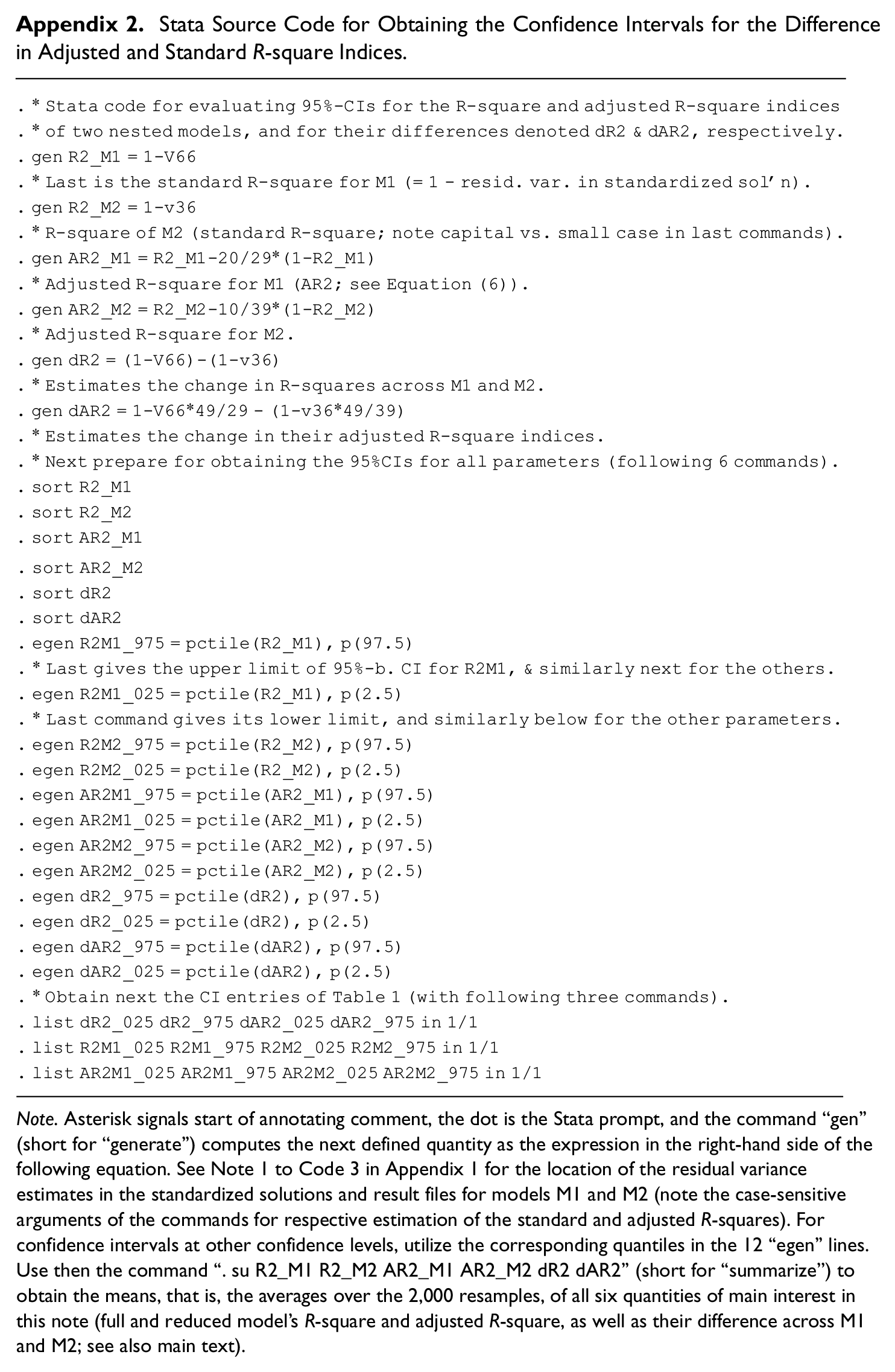
Stata Source Code for Obtaining the Confidence Intervals for the Difference in Adjusted and Standard R-square Indices.

. * Stata code for evaluating 95%-CIs for the R-square and adjusted R-square indices
. * of two nested models, and for their differences denoted dR2 & dAR2, respectively.
. gen R2_M1 = 1-V66
. * Last is the standard R-square for M1 (= 1 - resid. var. in standardized sol’n).
. gen R2_M2 = 1-v36
. * R-square of M2 (standard R-square; note capital vs. small case in last commands).
. gen AR2_M1 = R2_M1-20/29*(1-R2_M1)
. * Adjusted R-square for M1 (AR2; see Equation (6)).
. gen AR2_M2 = R2_M2-10/39*(1-R2_M2)
. * Adjusted R-square for M2.
. gen dR2 = (1-V66)-(1-v36)
. * Estimates the change in R-squares across M1 and M2.
. gen dAR2 = 1-V66*49/29 - (1-v36*49/39)
. * Estimates the change in their adjusted R-square indices.
. * Next prepare for obtaining the 95%CIs for all parameters (following 6 commands).
. sort R2_M1
. sort R2_M2
. sort AR2_M1
. sort AR2_M2
. sort dR2
. sort dAR2
. egen R2M1_975 = pctile(R2_M1), p(97.5)
. * Last gives the upper limit of 95%-b. CI for R2M1, & similarly next for the others.
. egen R2M1_025 = pctile(R2_M1), p(2.5)
. * Last command gives its lower limit, and similarly below for the other parameters.
. egen R2M2_975 = pctile(R2_M2), p(97.5)
. egen R2M2_025 = pctile(R2_M2), p(2.5)
. egen AR2M1_975 = pctile(AR2_M1), p(97.5)
. egen AR2M1_025 = pctile(AR2_M1), p(2.5)
. egen AR2M2_975 = pctile(AR2_M2), p(97.5)
. egen AR2M2_025 = pctile(AR2_M2), p(2.5)
. egen dR2_975 = pctile(dR2), p(97.5)
. egen dR2_025 = pctile(dR2), p(2.5)
. egen dAR2_975 = pctile(dAR2), p(97.5)
. egen dAR2_025 = pctile(dAR2), p(2.5)
. * Obtain next the CI entries of Table 1 (with following three commands).
. list dR2_025 dR2_975 dAR2_025 dAR2_975 in 1/1
. list R2M1_025 R2M1_975 R2M2_025 R2M2_975 in 1/1
. list AR2M1_025 AR2M1_975 AR2M2_025 AR2M2_975 in 1/1

Note. Asterisk signals start of annotating comment, the dot is the Stata prompt, and the command “gen” (short for “generate”) computes the next defined quantity as the expression in the right-hand side of the following equation. See Note 1 to Code 3 in Appendix 1 for the location of the residual variance estimates in the standardized solutions and result files for models M1 and M2 (note the case-sensitive arguments of the commands for respective estimation of the standard and adjusted R-squares). For confidence intervals at other confidence levels, utilize the corresponding quantiles in the 12 “egen” lines. Use then the command “. su R2_M1 R2_M2 AR2_M1 AR2_M2 dR2 dAR2” (short for “summarize”) to obtain the means, that is, the averages over the 2,000 resamples, of all six quantities of main interest in this note (full and reduced model’s R-square and adjusted R-square, as well as their difference across M1 and M2; see also main text).

Author Note

We are indebted to G. A. Marcoulides and K. M. Marcoulides for valuable discussions on latent variable methods and their applications, as well as to two anonymous Referees for valuable and critical comments on an earlier version of this paper, which contributed to its significant improvement.

Declaration of Conflicting Interests

The author(s) declared no potential conflicts of interest with respect to the research, authorship, and/or publication of this article.

Funding

The author(s) received no financial support for the research, authorship, and/or publication of this article.

ORCID iDs

Tenko Raykov

Christine DiStefano

Notes

References

Agresti

(2018). Statistical methods for the social sciences. Pearson.

Apostol

(2006). Calculus. Wiley.

Bollen

K. A.

(1989). Structural equations with latent variables. Wiley.

Casella

Berger

J. O.

(2002). Statistical inference. Wadsworth.

Draper

N. R.

Smith

(1998). Applied regression analysis. Wiley.

Efron

Tibshiriani

(1993). An introduction to the bootstrap. Chapman & Hall.

Field

(2018). Discovering statistics using IBM SPSS Statistics. Sage.

Geiser

(2013). Data analysis with Mplus. Guildford.

Harrell

F. E.

(2015). Regression modeling strategies. Springer.

10.

Jöreskog

K. G.

Sörbom

(1996). LISREL8 user’s reference guide. Scientific Software.

11.

Judd

C. M.

McClelland

G. H.

Ryan

C. S.

(2017). Data analysis: A model comparison approach. Routledge.

12.

Marcoulides

K. M.

Raykov

(2019). Evaluation of variance inflation factors in regression models using latent variable modeling methods. Educational and Psychological Measurement, 79, 874–882.

13.

Muthén

B. O.

(2002). Beyond SEM: General latent variable modeling. Behaviormetrika, 29, 81–117.

14.

Muthén

B. O.

Muthén

L. K.

Asparouhov

(2016). Regression and mediation analysis with Mplus. Muthen & Muthen.

15.

Muthén

L. K.

Muthén

B. O.

(2025). Mplus user’s guide. Muthén & Muthén.

16.

Rabe-Hesketh

Skrondal

(2022). Multilevel and longitudinal modeling using Stata. Stata Press.

17.

Raykov

(2001). Testing multivariable covariance structure and means hypotheses via structural equation modeling. Structural Equation Modeling, 8, 224–256.

18.

Rhemtulla

Brosseau-Liard

P. É.

Savalei

(2012). When can categorical variables be treated as continuous? A comparison of robust continuous and categorical SEM estimation methods under suboptimal conditions. Psychological Methods, 17, 354–373.

19.

Schmidt

F. L.

(1996). Statistical significance testing and cumulative knowledge in psychology: Implications for training of researchers. Psychological Methods, 1, 115–129.