When Cluster-Robust Inferences Fail

Abstract

Although cluster-robust standard errors (CRSEs) are commonly used to account for violations of observations independence found in nested data, an underappreciated issue is that there are several instances when CRSEs can fail to properly maintain the nominally accepted Type I error rate. These situations (e.g., analyzing data with imbalanced cluster sizes) can readily be found in various types of education-related datasets and are important to consider when computing statistical inference tests when using cluster-level predictors. Using a Monte Carlo simulation, we investigated these conditions and tested alternative estimators and degrees of freedom (df) adjustments to assess how well they could ameliorate the issues related to the use of the traditional CRSE (CR1) estimator using both continuous and dichotomous predictors. Findings showed that the bias-reduced linearization estimator (CR2) and the jackknife estimator (CR3) together with df adjustments were generally effective at maintaining Type I error rates for most of the conditions tested. Results also indicated that the CR1 when paired with df based on the effective cluster size was also acceptable. We emphasize the importance of clearly describing the nested data structure as the characteristics of the dataset can influence Type I error rates when using CRSEs.

Keywords

clustered data cluster robust standard errors degrees of freedom effective sample size

Nested (or clustered) data are commonly encountered in educational research (e.g., students within schools), which violates a well-known regression assumption of observation independence (Cohen et al., 2003). Ignoring or not accounting for the dependent nature of clustered data can result in incorrect statistical inference tests for cluster-level predictors, resulting in higher Type I errors or erroneous claims of statistical significance (Baldwin et al., 2005; Murray et al., 2004). Although various modeling approaches have been developed for the analysis of dependent data (Huang, 2016) such as multilevel modeling (Laird & Ware, 1982) or using a generalized estimating equations (Liang & Zeger, 1986) approach, cluster-robust standard errors (CRSEs) have been routinely applied, especially in fields such as applied econometrics (Chiang et al., 2025) and epidemiology (Mansournia et al., 2021), to account for the presence of clustered data.

Developments in CRSEs can be traced back to the original formulation of Liang and Zeger (1986), and CRSEs are often applied to account for clustered data when using ordinary least squares (OLS) or generalized linear models (GLMs). Although methods such as multilevel models (MLMs) are powerful and flexible, MLMs have strong assumptions that when violated (e.g., correct specification of random effects) can result in biased estimates (Huang & Zhang, 2025; Huang, Wiedermann, & Zhang, 2023). As a result, CRSEs can also be used with MLMs (Huang, Wiedermann, & Zhang, 2023) and when using a GEE approach (Huang, 2022) to account not just for clustering, but for any form of unobserved heterogeneity. Over the years, several articles (e.g., Esarey & Menger, 2019; Weiss, 2024; Young, 2016) have investigated the use of CRSEs and degrees of freedom (df) adjustments in relation to statistical inference tests with clustered data.

However, it may not be widely recognized (or underappreciated) that there are several instances where using CRSEs can still result in incorrect statistical inference tests (Cameron & Miller, 2015; MacKinnon et al., 2023a). A review of empirical research, even from well-known journals such as the American Economic Review and Econometrica (from 2020 to 2021) showed that a nontrivial percent (77%) of published research had used CRSEs under certain conditions, which raises questions related to the validity of their findings (Chiang et al., 2025). As CRSEs have been used in various types of models (e.g., MLMs, GLMs), being able to recognize the conditions where CRSEs may not be adequate is then of importance if researchers are concerned about making correct statistical inferences.

The article is outlined as follows: We first begin by providing a brief background on the traditional CRSE. Next, we describe several instances where the use of CRSEs may not maintain the nominally stated Type I error rate for cluster-level predictors. Third, we discuss alternative approaches that involve both the computation of the CRSEs and the choice of df. Fourth, we conduct a Monte Carlo experiment where we replicate conditions where traditional CRSEs will fail and then test alternative approaches if they fare any better. We conclude with a discussion and summary of results.

Brief Background on Cluster-Robust Standard Errors

In matrix form, the linear regression model is written as $y = X β + ε$ , where $y$ is an N× 1 vector of outcomes, with N observations. The matrix $X$ is an N×k design matrix containing the predictor variables and k is the total number of predictors (including the intercept). The vector $β$ is a k× 1 vector of regression coefficients and $ε$ is an N× 1 vector of error (disturbance) terms. The regression coefficients can be estimated using OLS resulting in $\hat{β} = {(X^{'} X)}^{- 1} X' y$ .

Standard errors can be estimated using $Var (\hat{β}) = {(X^{'} X)}^{- 1} X^{'} \hat{Ω} X {(X^{'} X)}^{- 1}$ , where $\hat{Ω}$ is an estimated N×N variance/covariance matrix of the error terms. In a standard OLS model, $\hat{Ω} = {\hat{σ}}^{2} I$ , where I is an N×N identity matrix; ${\hat{σ}}^{2} = \frac{{\hat{ε}}^{'} \hat{ε}}{n - k}$ , where $\hat{ε}$ is a vector of residuals $\hat{ε} = y - X \hat{β}$ . Using a constant ${\hat{σ}}^{2}$ assumes that variability is homogeneous. The standard errors are the square roots of the diagonal of the $Var (\hat{β})$ matrix.

Extended to a clustered data setting, the variance/covariance matrix of the coefficients can be estimated using

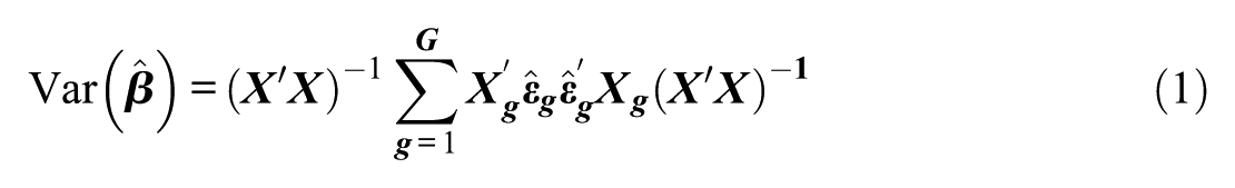
Var (\hat{β}) = {(X' X)}^{- 1} \sum_{g = 1}^{G} X_{g}^{'} {\hat{ε}}_{g} {\hat{ε}}_{g}^{'} X_{g} {(X' X)}^{- 1}

(1)

where now, the term in the middle is estimated per cluster g and then summed together (G is the total number of clusters). In this formulation, $X_{g}$ is a cluster-specific design matrix and ${\hat{ε}}_{g}$ is a cluster-specific vector of residuals. Without any form of adjustments (e.g., to account for a few clusters), this is referred to as the Liang and Zeger (1986) CRSE or CR0.

The unadjusted CR0 is the default CRSE estimator used in procedures when using generalized estimating equations (Liang & Zeger, 1986) or in software (with some modifications to account for random effects) such as HLM (Raudenbush & Congdon, 2021). However, finite-sample modifications (due to having small G) can be used to slightly reduce the downward bias of the CRSE. Different software may implement adjustments to account for a limited number of clusters such as scaling the $Var (\hat{β})$ matrix by a factor of $\frac{G}{G - 1}$ such as in SAS or the sandwich package in R (Zeileis, 2006).¹ With clustered data and when using robust maximum likelihood estimation for procedures when fitting structural equation models (SEMs) using lavaan (Rosseel, 2012) or Mplus (Muthén & Muthén, 1998), the equivalent of the CR0 × small sample correction is estimated.

In applied econometrics, the most widely used CRSE is the CR1 (MacKinnon et al., 2023b), which is the CR0 multiplied by a scaling factor of $\frac{G}{G - 1} \times \frac{N - 1}{N - k}$ (see Cameron & Miller, 2015). As G gets larger, the adjustments are negligible, though may count more when G is small, but will not fully eliminate the bias of the CRSE with a few clusters. The CR1 is the default estimator when using Stata and R (when using the sandwich package).

When Do CRSEs Fail?

Analyzing Data With Only a Few Clusters

The most commonly mentioned limitation when using the traditional CR0 estimator is that it works well when the number of clusters is reasonably large and performs poorly when there are only a few clusters (Bell & McCaffrey, 2002; Cameron & Miller, 2015). Conventional guidelines indicate that when there are around 20 (Muthen, 2005)² or 40 (Angrist & Pischke, 2008) clusters, the use of CRSEs should not be an issue. With a limited number of clusters, CR0 standard errors are well-known to be underestimated for cluster-level coefficients (Bell & McCaffrey, 2002). However, less known is that inferences may still be incorrect even in some situations when there are even 100 or 200 clusters (Djogbenou et al., 2019; MacKinnon et al., 2023a). Being able to discern when situations may be problematic is thus of importance to the applied researcher.

Using Inappropriate df

Although standard errors are important, when p-values and confidence intervals are obtained, this is done in conjunction with the t-critical values based on the df used. Traditional OLS df are determined by the sample size and the number of predictors; the t-critical value is based on N−k. However, with clustered data, researchers may have hundreds of observations but only a limited number of clusters actually present (e.g., 600 students nested within 20 schools).

To obtain t-critical values of ±1.96 when constructing confidence intervals, this assumes a large number of clusters (i.e., G = ∞) and that the test statistic follows a normal distribution. Certain software (e.g., Mplus) may assume by default a z-critical value of 1.96. However, if t-tests for cluster-level predictors are done using the traditional df of N−k, then the critical values may be too low when there are only a few clusters. As indicated by Elff et al. (2016, p. 16) “it is very misleading to construct p-values, hypothesis tests, and confidence intervals for the coefficients of upper-level variables using the assumption that the corresponding t-statistic (i.e., the coefficient estimate divided by its standard error) follows the standard normal distribution.”

Instead, critical values can be constructed based on the number of G clusters and often, G− 1 (Cameron & Miller, 2015) or G−L− 1 (Donald & Lang, 2007) where L represents the number of cluster-level predictors, can be used (Stata uses G− 1 by default). If there are many clusters, the difference in critical values may be trivial (e.g., with G = 200, the t-critical values are ±1.97). However, when there are fewer clusters, the choice of df can have more consequential results, perhaps even more so than the choice of the CRSE alone (Pustejovsky & Tipton, 2018; Young, 2016). Basing the df on G instead of N is more conservative (as long as G≠N) but can still result in higher Type I errors with only a few clusters (MacKinnon & Webb, 2017).

Having Clusters That Wildly Vary in Size

Additional issues related to the adequate number of clusters for CRSEs stem from what is referred to as cluster heterogeneity (Carter et al., 2017) that can be brought about as a result of large imbalances in cluster size. As a result of cluster heterogeneity, the effective number of clusters, referred to as G*, is often much less than the observed number of clusters G (we discuss computations for G* in a succeeding section). Large differences in the number of observations per cluster can also have an effect on Type I errors (MacKinnon et al., 2023a).

A classic example of this type of dataset comes from applied economics and involves studies that compare different outcomes across 50 U.S. states (e.g., based on the introduction of some policy). If using data representative of the population of each state, California accounts for 12% of the total U.S. population and 20 states (e.g., Iowa, Wyoming) each comprise less than 1% of the U.S. population. Although in this case, G = 50, the results of one cluster may have a disproportional effect compared to the rest of the sample, which will then influence the regression coefficients. However, when computing the CRSE, each cluster contributes equally to the variance of the coefficients. As indicated by Bell and McCaffrey (2002, p. 7), “greater bias appears to occur when certain [clusters] account for most of the variability in the covariates and have disproportionate impact on the determination of the [the regression coefficients].” The CR1 performs well with relatively balanced cluster sizes but has higher Type I error rates with the presence of extremely large clusters (relative to the rest of the sample) (MacKinnon & Webb, 2017).

School-based research may also find situations with large variations in cluster sizes. This may be less of an issue with properly controlled experimental studies, though it may become increasingly more common with secondary data analysis with the availability of statewide longitudinal data systems (SLDS) and other statewide administrative databases. For example, in the Virginia Secondary School Climate Survey (Cornell et al., 2017) in 2017, there were 85,762 middle-school respondents from 410 schools. The mean number of respondents per school was 209 students, with a range from 7 to 1,620. Twenty-five percent of the schools had fewer than 68 respondents, and there were 9 schools with more than 1,000 respondents.

Of importance as well is that variation in cluster sizes can be represented as a coefficient of variation (cv), which is the ratio of the standard deviation of the cluster sizes to the mean of the cluster sizes ( $\bar{N_{g}}$ ). For a completely balanced sample where every cluster has the same size, cv_Ng = 0. In a study of cluster randomized controlled trials, Eldridge et al. (2006) reported an average cv_Ng = 0.65. In the preceding examples, the country-wide dataset using states as clusters had a cv_Ng of 1.12, while the school-based example had a cv_Ng of 1.18 (both of which represent high variability).

Having Too Few (or Too Many) Treated Clusters

CRSEs may also fail to provide accurate statistical inference tests in the presence of too few or too many “treated” clusters. As indicated by Cameron and Miller (2015),

Problems arise if most of the variation in the regressor is concentrated in just a few clusters, even when G is sufficiently large. This occurs if the key regressor is a cluster-specific binary treatment dummy and there are few treated groups. (p. 349)

In this case, a treated cluster has predictor T = 1 if in a treatment condition and T = 0 if in a control condition, and this is assigned at the cluster level (all observations in the same cluster have the same measure of T). However, in the case where there are only a limited number of clusters that get treated (e.g., 2 out of 20 clusters have T = 1), then Type I errors are larger than the nominally accepted .05 (MacKinnon & Webb, 2017).³

In an educational context, when doing school-based research, binary cluster-level predictors are not uncommon. For example, if comparing the performance of students attending public or private schools, school type is a cluster-level predictor. Often, in large-scale international assessments, data are collected from public and private schools and depending on the country, the number of private schools sampled is far less than public schools. In the Programme for International Student Assessment (PISA) 2018 dataset (OECD, 2020), in the U.S. sample, there were only 10 private schools compared to 138 public schools or 6.7%.

Dealing With the Deficiencies of Traditional CRSEs

Although several specific situations have been identified when cluster robust inferences may fail, a few approaches have been proposed that may ameliorate such issues. For the current article, we focus on using an alternative cluster-robust estimator and using different df estimation techniques (which may not be commonly used).

Alternative Estimator: The CR2

Alternative variants of the CR0 CRSE have been developed over the years to account for the presence of a few clusters (see Cameron & Miller, 2015). One CRSE variant that has received more recent attention is the CR2 adjustment (Huang, 2022; Imbens & Kolesar, 2016; Pustejovsky, 2018) or the bias-reduced linearization (BRL) estimator of Bell and McCaffrey (2002). Instead of the variance/covariance matrix estimated using equation (1), adjusted residuals are included so that $Var (\hat{β})$ is estimated using

{V a r}_{C R 2} (\hat{β}) = {(X^{'} X)}^{- 1} \sum_{g = 1}^{G} X_{g}^{'} A_{g} {\hat{ε}}_{g} {\hat{ε}}_{g}^{'} A_{g} X_{g} {(X^{'} X)}^{- 1},

(2)

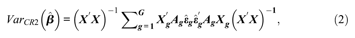
where an adjustment matrix, $A_{g}$ , is included in the form of

A_{g} = {(I_{Ng} - H_{g})}^{- 1 / 2},

(3)

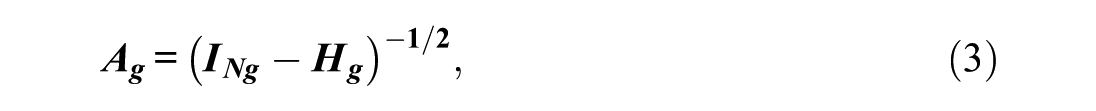
where $I_{Ng}$ is an identity matrix based on the number of observations in cluster g and $H_{g}$ is a cluster-specific projection (“hat”) matrix:

H_{g} = X_{g} {(X^{'} X)}^{- 1} X_{g}^{'} .

(4)

The inverse of the symmetric square root of the quantity has been shown to help reduce the estimated standard error bias when residuals within the cluster are correlated and the cluster-level hat matrix reduces bias from overrepresented clusters (Bell & McCaffrey, 2002). As a result, the CR2 adjusts for leverage and improves inferences in the presence of unbalanced clusters. Even though the CR2 estimator has been available for over two decades, it has seen limited use in applied research though recent studies have found that it performs well (i.e., less biased, lower Type I errors), even with a limited number of clusters compared to the CR0 (Huang & Li, 2022; Pustejovsky & Tipton, 2018). MacKinnon and Webb (2017) considered the CR2 adjustment in their simulation investigating solutions to cluster heterogeneity, but given their interest in large samples (e.g., >500,000 observations), which required extensive computational time and memory (i.e., obtaining the inverse symmetric square roots of the adjustment matrices can be challenging), they decided it was not feasible to study its performance. Niccodemi et al. (2020) presented a faster formulation of the CR2 (in Appendix A of their paper) which requires an inversion of smaller k×k matrices instead which would circumvent this problem.

Alternative Estimator: The CR3

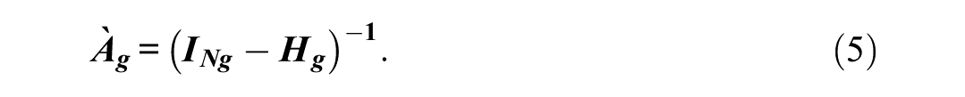
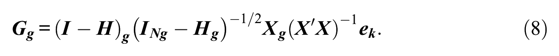
Bell and McCaffrey (2002), in the same article that introduced the CR2, presented the formulation for the jackknife operator also referred to as the CR3 (MacKinnon & Webb, 2017). The formulation of the CR3 is the same as the CR2 with the exception that instead of equation (3) which requires the inverse of the symmetric square root, only the inverse is required for the adjustment matrix:

À_{g} = {(I_{Ng} - H_{g})}^{- 1} .

(5)

MacKinnon et al. (2023b) also included a scaling factor of $\frac{G - 1}{G}$ applied to the variance/covariance matrix such that

{V a r}_{C R 3} (\hat{β}) = \frac{G - 1}{G} {(X^{'} X)}^{- 1} \sum_{g = 1}^{G} {X^{'}}_{g} À_{g} {\hat{ε}}_{g} {\hat{ε}}_{g}^{'} À_{g} X_{g} {(X^{'} X)}^{- 1} .

(6)

Although the CR2 has often been recommended (Imbens & Kolesar, 2016; Pustejovsky & Tipton, 2018), others have suggested the use of the CR3 as well (MacKinnon et al., 2023a, 2023b) indicating that it performs as well as or better than the CR2 (in some situations) and is computationally less demanding. Hansen (2025) recommended its routine use compared to the CR1 estimator and indicated that the CR3 will tend to be conservative (i.e., underreject the null) which was also reported by Bell and McCaffrey (2002).

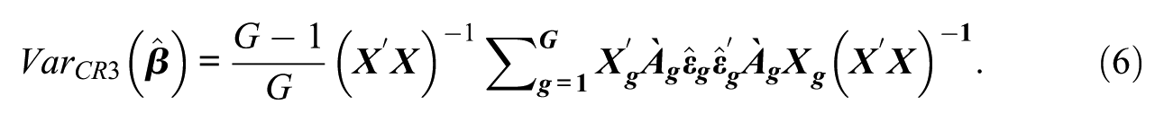
As a jackknife estimator, which uses a “leave-one-out” resampling process, MacKinnon et al. (2023b) presented an alternative formulation of the CR3. The OLS estimates of $β$ are $\hat{β} = {(X^{'} X)}^{- 1} X' y$ and instead of leaving out one observation (as in the standard jackknife), each cluster is omitted in turn such that: ${\hat{β}}_{g} = {(X^{'} X - X_{g}^{'} X_{g})}^{- 1} (X^{'} y - X_{g} y_{g}), g = 1, \dots, G$ . After G estimates of $\hat{β}$ are computed,

{V a r}_{C R 3} (\hat{β}) = \frac{G - 1}{G} \sum_{g = 1}^{G} ({\hat{β}}_{g} - \hat{β}) {({\hat{β}}_{g} - \hat{β})}^{'} .

(7)

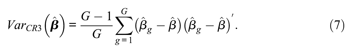
Results using equations (6) and (7) are the same though the latter is more efficient as it does not depend on the adjustment matrix which can be large. In R, packages such as sandwich (Zeileis, 2006) and clubSandwich (Pustejovsky, 2018) compute the CR3 without the scaling factor. Niccodemi et al. (2020) also showed an efficient way to compute the CR3 in addition to the CR2, and Hansen (2025) showed computations for the CR3 using a generalized inverse instead.

Alternative df: Using the Effective Number of Clusters Versus Observed Number of Clusters

Clusters that vary in size can lower what is referred to as the effective number of clusters. At a basic level, from the survey sampling literature (Asparouhov, 2006; Potthoff et al., 1992), the effective number of clusters can be computed using: $G^{*} = {(\sum_{g = 1}^{G} N_{g})}^{2} / (\sum_{g = 1}^{G} N_{g}^{2})$ , where $N_{g}$ refers to the number of observations in cluster g.⁴ This approach, although this takes into consideration the variation in cluster sizes, does not consider differences in the covariates in each cluster (i.e., there are differences in the characteristics of the members in each group and are not completely homogeneous). Instead, Carter et al. (2017) and Lee and Steigerwald (2018) developed an alternative formulation of G* which takes into consideration the covariates in each cluster. Based on Carter et al. (2017) and Lee and Steigerwald (2018): $G^{*} = \frac{G}{1 + Γ}$ where $Γ = \frac{1}{G} \sum_{g = 1}^{G} {(\frac{γ_{g} - \bar{γ}}{\bar{γ}})}^{2}$ . Using $a$ as a selection vector for the coefficient of interest, $γ_{g} = a' {(X^{'} X)}^{- 1} (X_{g}^{'} i_{g} i_{g}^{'} X_{g}) {(X^{'} X)}^{- 1} a$

In the computation of $γ_{g}$ , Carter et al. (2017) suggested using a 1-by- $N_{g}$ vector of ones for $i_{g}$ to represent a conservative estimate which imposes a perfect within-cluster correlation (i.e., the variable does not vary within the group, which is typical of cluster-level predictors). As a result of using the cluster-specific design matrices, G* varies depending on the covariates included in the model. The quantity G* can be computed using the clusteff (Lee & Steigerwald, 2018) module in Stata or the effClust (Ritter, 2024) package in R. The summclust function, which uses an alternative formulation for G*, is also available in Stata (MacKinnon et al., 2023b).⁵ Although Carter et al. formulated the use of G* primarily as a diagnostic, they did not specifically propose its use as an alternative df measure (see Cameron et al., p. 348) though using G* is reasonable.

Comparing G to G*-1 can be informative (i.e., comparing the observed number of clusters to the effective number of clusters). For example, Carter et al. (2017) used the well-known Tennessee Project Star (Achilles et al., 2008) dataset analyzed by Krueger (1999). In the dataset, Carter et al. reported that there were 318 kindergarten teachers (the number of clusters G), but the number of students varied across classrooms from 9 to 27 (M = 18, s² = 15.7). Computing the effective number of clusters, G* = 192, a reduction of 40%.⁶ In this case, the coefficient of variation was a modest cv = 0.22.

Alternative df: Using Satterthwaite df Approximations

In the same manuscript where they proposed the CR2 estimator, Bell and McCaffrey (2002) also provided a Satterthwaite df adjustment given by $d f_{BM} = (Σ_{g = 1}^{G} λ_{g})^{2} / Σ_{g = 1}^{G} λ_{g}^{2}$ (see Cameron & Miller, 2015; Imbens & Kolesar, 2016). The $λ$ s are the eigenvalues of a $G^{'} G$ matrix where G is an N×G matrix. The G matrix is a result of stacking G_g columns where

G_{g} = {(I - H)}_{g} {(I_{Ng} - H_{g})}^{- 1 / 2} X_{g} {(X' X)}^{- 1} e_{k} .

(8)

The first term, ${(I - H)}_{g}$ , is an N×N_g matrix where both I and H are N×N identity and hat matrices. The subscript g indicates that only the columns with observations that belong to group g are selected, resulting in N_g columns. The second term ${(I_{Ng} - H_{g})}^{- 1 / 2}$ is the same adjustment matrix in equation (3), which is an N_g×N_g matrix. The third term, $X_{g} {(X' X)}^{- 1}$ , results in an N_g×k matrix. The final term $e_{k}$ is a k× 1 indicator (i.e., selector) vector of k predictors, which specifies which predictor to compute the df for (e.g., in a model with four predictors, to compute the df for the last coefficient, $e_{k}$ would be (0, 0, 0, 1). Unlike df computations based simply on sample size (e.g., N −k, G − 1), df_BM will change depending on the model and the data used as both the matrices X and H are used in the computations.

The Current Study

As the issues related to the fallibility of CRSEs are based on having a few clusters, large imbalances in cluster sizes, and analyzing clustered treatments with low prevalence rates, we conducted a simulation to assess the performance of the CR1, CR2, and CR3 together with df variations using dfG-1, dfG*-1, dfBM. Although prior studies have investigated the use of the CR2 with dfBM (e.g., Huang & Li, 2022), the combination of factors directly related to the issues with statistical inference tests were not directly manipulated (e.g., cluster sizes were not largely unbalanced). MacKinnon and Webb (2017) investigated the use of G*− 1 vs. G− 1 as a df alternative and found that using G* performed better than just using G, but their simulation was limited in terms of the number of clusters used (e.g., 50 and 100) and did not consider dfBM nor the CR2. As the CR2 and CR3 account for cluster heterogeneity and the choice of df can be consequential (Pustejovsky & Tipton, 2018), testing out the combinations of CRSEs and df in situations where inferences may fail can provide valuable insights into the robustness of statistical conclusions under different assumptions.

Method

Data Generating Process (DGP)

To investigate the conditions where cluster-robust inferences may fail and assess approaches that may ameliorate the issue, we conducted a Monte Carlo simulation using R (R Core Team, 2025). We simulated a two-level linear model (e.g., students within schools) with dependent variable Y _ig representing the outcome Y for observation i in cluster/group g such that $Y_{ig} = β_{0} + β_{1} T_{g} + β_{2} X_{1 g} + u_{0 g} + r_{ig} .$ The variable $T_{g}$ (a “treatment” indicator) was a second-level dichotomous variable which is constant within the group. The variable $X_{1 g}$ is a continuous cluster-level predictor, assumed to follow a standard normal distribution: $X_{1 g} ~ N (0, 1)$ . All $β s$ were set to zero and two error terms, $u_{0 g}$ and $r_{ig}$ , were included which represented variability at the group and individual levels, respectively. Both error terms followed a normal distribution such that $u_{0 g} ~ N (0, ρ)$ and $r_{ig} ~ N (0, 1 - ρ)$ resulting in Y _ig having a unit variance (where $ρ < 1$ ).

As we were interested in situations where cluster robust inferences may be problematic (based on Type I error rates), which is why $β_{1} = β_{2} = 0$ ), we manipulated several factors including number of clusters ( G = 20, 40, 60, 80, 100), the number of observations per cluster (Ng = 30, 100), the intraclass correlation coefficients ( ICC = .10, .30), the prevalence rate of the binary predictor ( prevalence = .10, .30, .50), and the coefficient of variation which determines the degree of imbalance of the cluster sizes ( cv = 0.10, 0.65, 1.10). All factors were fully crossed resulting in 180 conditions. For each condition, 2,000 replications were used.

The ICCs represent what may be considered typical ICCs in an educational context (see Hedges & Hedberg, 2007) with higher ICCs indicating a higher proportion of a cluster-level effect and is directly controlled by the value of $ρ$ (i.e., .10 or .30) resulting in a unit variance of Y _ig . Given that the number of clusters, the prevalence rate of binary cluster-level variables, and the imbalance in cluster size directly contributes to the fallibility of CRSEs, these are manipulated in the simulation. The number of clusters represents cases that may represent a range of a few (G = 20) to many clusters (G = 100) as seen in other simulations (e.g., Bell & McCaffrey, 2002; MacKinnon & Webb, 2017). The number of observations per cluster may be typical in education when selecting students from a class or an entire school. Of note as well is that with the prevalence rates for the binary variable (where .50 indicates balanced groups), for .10 and .30, their complements are .90 and .70 so are not included (i.e., the issue of having too few clusters with a condition is the same as having too many). With each replication, prevalence×G clusters are randomly selected and assigned T = 1 with the rest of the groups being assigned T = 0. In this manner (instead of drawing T from a binomial distribution), the prevalence of T is exact per replication. Imbalances are based on the coefficient of variation (cv) where 0.10 signifies minimal imbalance (0 is completely balanced), 0.65 is typical of imbalances in cluster-randomized controlled trials (Eldridge et al., 2006), and 1.10 represents high variability situations such as the case of analyzing U.S. state datasets. The number of observations per G clusters was drawn from a random normal distribution with mean Ng and a standard deviation of N_g×cv. Clusters with fewer than five observations were set to a size of five. The cv is a common parameter that researchers (e.g., Li & Redden, 2015; Martin et al., 2019) use in simulations to manage and quantify the variability (imbalance) of nonuniformly distributed cluster sizes.

For each simulated dataset, the effects of T and $X_{1 g}$ were evaluated using different approaches and given that $β_{1} = β_{2} = 0$ , we would expect the coefficients to be statistically significant 5% out of the 2,000 replications. The coefficients of interest were evaluated using: 1) the CR1 estimator with dfG-1; 2) a two-level random intercept model (which matches the DGP); 3) the CR1 estimator with dfG*-1; 4) the CR1 estimator with dfBM; and 5) the CR2 estimator with dfG*-1; 6) the CR2 estimator with dfBM; and 7) the CR3 estimator with dfG*-1 (as done by MacKinnon et al., 2023b). The CR1:dfG-1 is used to assess how much this estimator may be off given the conditions and the random-intercept model (estimated using restricted maximum likelihood) is used only as a point of comparison. The random intercept model is fit using the lmerTest package (Bates et al., 2015; Kuznetsova et al., 2017) and uses Satterthwaite df approximations, which have been effective at controlling Type I error rates in mixed models (Luke, 2017). If simulation conditions are working as expected, the CR1:dfG-1 should perform the worst, and the MLM should fit well (though we are unaware of other studies that specifically used an MLM with these more extreme conditions). Although other studies in applied econometrics (e.g., Hansen, 2025; MacKinnon & Webb, 2017) may consider alternatives such as wild cluster bootstrapping (WCB; Cameron et al., 2008; Roodman et al., 2019), WCB is not commonly used in education and psychology. We use Bradley’s (1978) liberal criterion to assess the robustness of the statistic using a threshold of 2.5% to 7.5% and Type I error rates beyond these bounds are deemed more problematic (resulting from over- or under-coverage).

Results

Type I Error Rates for the Cluster-Level Binary Predictor

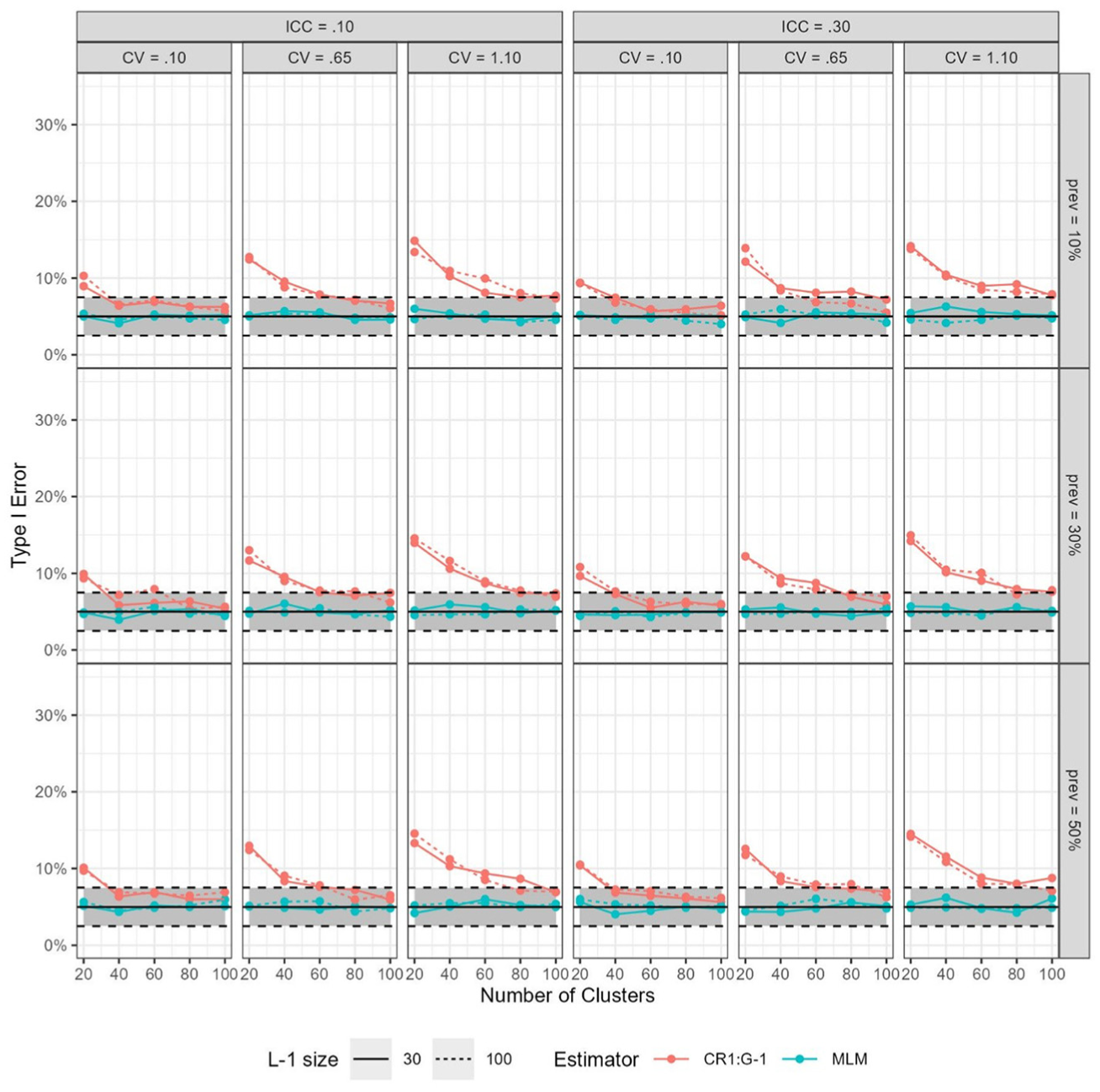
For the binary cluster-level predictor, Type I error rates are shown in Figure 1 for all conditions for models estimated using CR1:dfG-1 and MLM. The multilevel models all had Type I error rates within the noted thresholds of 2.5% to 7.5%, regardless of the condition manipulated.

Figure 1.

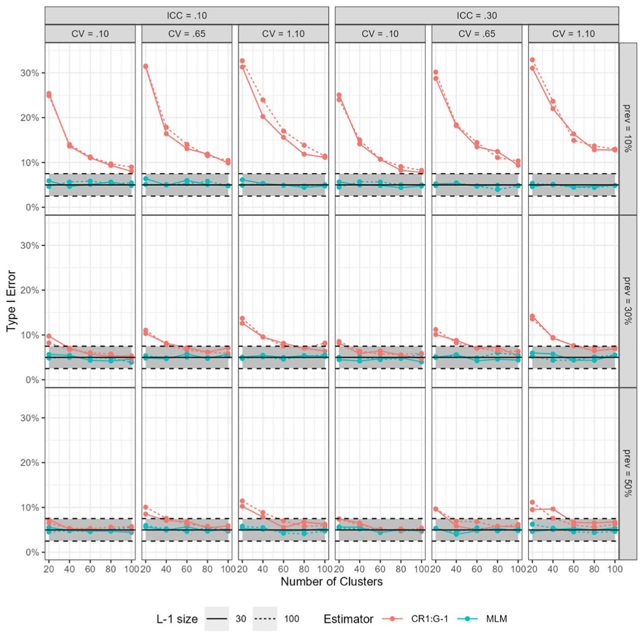
Type I Error Rates per Condition Using the CR1 Estimator and MLM (Multilevel Models) Using 2,000 Replications for the Level-2 Binary Predictor.

However, of all the conditions tested, the low-prevalence-rate condition (prev = 10%) had the largest effect in contributing to the extremely high rejection rates for the CR1:dfG-1 estimator. When prev = 10%, all of the CR1:dfG-1 Type I errors were above the 7.5% threshold and could be as high as around 35% (compared to the nominally expected 5%) in the prev = 10%, cv = 1.10, and G = 20 condition. Notably, in the prev = 10% condition, even with G = 100, Type I error rates could still be as high as 15% when cluster sizes were extremely imbalanced (cv = 1.10).

Even when prevalence rates were not as extreme (e.g., prev = 30%), rejection rates could still be higher than 5% for the CR1:dfG-1 estimator with G = 60, with the highly imbalanced condition. In the balanced condition where prev = 50%, Type I errors could still be higher when G was low and/or cv was high.

Alternative Estimators for the Binary Predictor

As the number of units per cluster (i.e., 30 vs.100) did not show a stark difference in Figure 1 (i.e., the dashed and solid lines were almost parallel to each other), for the alternative estimators, we show the results for Ng = 30 for clarity to avoid cluttering the plots. For the low-prevalence condition (prev = 10%), the CR1:dfBM could have Type I errors a little over 10% when G = 20 and cluster sizes were highly imbalanced (see Figure 2). Regardless of prevalence rates, the higher Type I error rates persisted when G = 20 and cluster sizes were extremely unbalanced (regardless of ICC) when using the CR1:dfBM.

Figure 2.

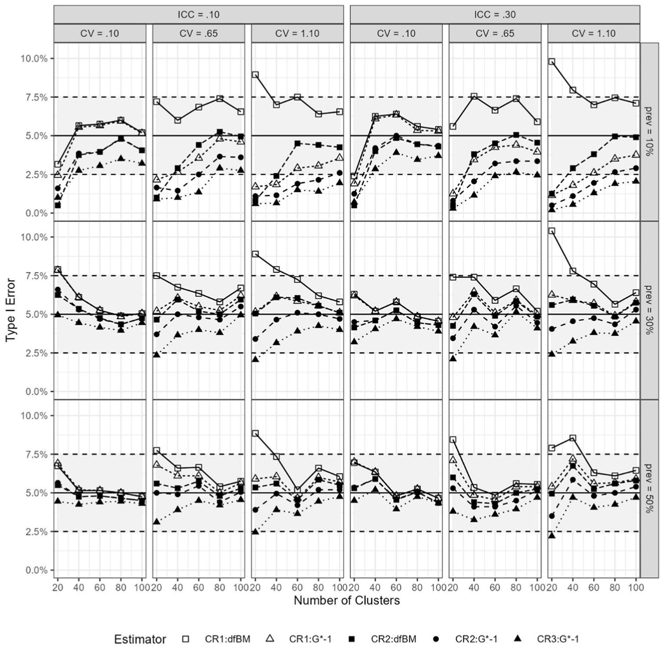
Type I Error Rates per Condition Using the CR1, CR2, and CR3 Estimators and Degrees of Freedom Adjustments Using 2,000 Replications for Level-2 Binary Predictor.

When the prevalence rates were ≥30%, the CR1:dfG*-1 and CR2 estimators had rejection rates that were generally in the acceptable established thresholds ranges. The CR3 estimator tended to be more conservative as well, with lower rejection rates compared to the other estimators.

However, in the low-prevalence-rate condition (prev = 10%), specifically when G = 20, Type I error rates could be too low (< 2.5%) for the other estimators. With more extreme imbalances in cluster sizes and prev = 10%, the CR3 tended to have low rejection rates, regardless of the number of clusters. The CR2:dfBM performed well in most conditions, except for when G = 20 and the prevalence rate was only 10%.

Type I Error Rates for the Cluster-Level Continuous Predictor

For the continuous predictor, Type I error rates could be too high for the CR1:dfG-1 estimator and rates were highest (e.g., 15%) when cluster sizes were extremely unbalanced (see Figure 3). The imbalance in cluster sizes was the main cause of the higher Type I error rates, regardless of all other conditions. With the case of the continuous predictor, unlike the binary predictor, the prevalence rates did not influence the rejection rates (as expected). Again, the multilevel model results were near the nominally stated 5%.

Figure 3.

Type I Error Rates per Condition Using the CR1 Estimator and MLM (multilevel models) Using 2,000 Replications for the Level-2 Continuous Predictor.

Alternative Estimators for the Continuous Predictor

Both the CR1:dfG*-1 and the CR2 estimators (regardless of dfBM or dfG*-1) had Type I errors that were within the generally established thresholds for all conditions (see Figure 4). However, with the CR1:dfBM, Type I error rates could still be too high when the imbalance in cluster sizes was moderate (cv = 0.65) to high (cv = 1.10). The CR3 also tended to have lower rejection rates when G = 20.

Figure 4.

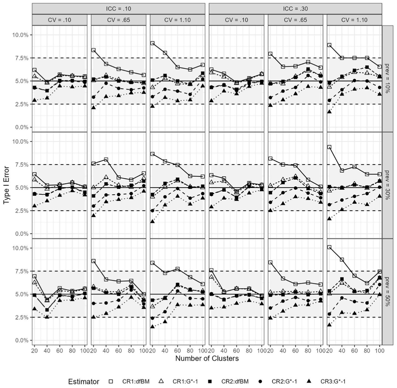
Type I Error Rates per Condition Using the CR1, CR2, and CR3 Estimators and Degrees of Freedom Adjustments Using 2,000 Replications for Level-2 Continuous Predictor.

Discussion

The current study investigated the performance of CRSEs under a range of conditions (using both continuous and dichotomous cluster-level predictors) commonly encountered in educational research, specifically in situations where the traditional use of CRSEs has been known to not perform as well. Using a Monte Carlo simulation, we evaluated the Type I error rates associated with the traditional CR1 estimator and the alternative CR2 and CR3 estimators used together with df adjustments based on the number of clusters (G), the effective number of clusters (G*), and the Satterthwaite approximation (dfBM). The findings underscore the importance of carefully considering both the estimator and the df when conducting inference tests with clustered data.

Our results revealed that the often-used CR1:dfG–1 estimator frequently produced inflated Type I error rates, particularly under conditions involving a small number of clusters, high variability in cluster sizes, and low prevalence rates when using a binary cluster-level predictor. The inflated rejection rates were also found when using continuous cluster-level predictors when there were few clusters and/or imbalanced cluster sizes (the “few treated clusters” does not apply to continuous predictors). These conditions are not uncommon in educational research, where studies may involve a limited number of schools or classrooms, where cluster-level predictor prevalence rates may be rare (e.g., alternative schools vs. traditional K-12 schools), and the number of observations per cluster may vary to a large degree. Although often, a rule-of-thumb for using CRSEs may only revolve around the number of clusters (e.g., using CRSEs with around 40 clusters is acceptable, Angrist & Pischke, 2008), we test a variety of conditions and show that even with 100 clusters, Type I error rates may still be too high, similar to findings of MacKinnon and Webb (2017). The large imbalance in cluster sizes exacerbates the Type I error rates for both continuous and binary cluster-level predictors.

However, the CR2 estimator, when paired with the dfBM approximation, demonstrated improved control over Type I error rates across most conditions. The exception would be when the prevalence rate for the binary predictor was low (i.e., 10%) and there were only 20 clusters. In those cases, the rejection rates were far too low (i.e., <2.5%). Though this may be of concern for cluster-randomized controlled trials that aim to reject the null hypothesis of equality, proper power analysis and practical experimental design will remedy this situation (i.e., researchers would not assign 2 out of 20 groups to a treatment condition as power would already be too low, not unless planned effect sizes were extremely large). With a continuous cluster-level predictor, the CR2:dfBM had near the nominally acceptable 5% for all conditions tested. The CR3 estimator was the most conservative estimate as a result of having the lowest Type I error rates among all estimators.

Although researchers have been warned about using the CR1 estimator with a limited number of clusters (e.g., Cameron & Miller, 2015), our findings show that, depending on the df used, acceptable Type I rates are possible. It should be clear that using the naïve G–1 should not be used, but then the CR1:dfBM can still result in higher Type I error rates as well with a binary predictor, with a few clusters, and imbalanced cluster sizes. The Type I error rates for the CR1 with G– 1 could be used, as long as cluster sizes are relatively balanced (i.e., cv ≤ 0.10), and this applies to both continuous and dichotomous cluster-level predictors.

One approach that has not seen much use would be to use the G*-1 as the df instead of G-1. Using G* in the df computation resulted in more conservative and often more accurate inferential tests. The CR1:dfG*-1 had very similar performance to the CR2:dfBM estimator for both the continuous and binary cluster-level predictors. However, like the CR2:dfBM and the CR3, the CR1:dfG*-1 could have Type I error rates that were far too low when G = 20 (MacKinnon & Webb, 2017), and the interest was in a binary predictor. An advantage of using the CR1:dfG*-1 estimator over the CR2:dfBM is that the CR1:dfG*-1 is less computationally demanding (i.e., it is easier to compute) and does not require computing the inverse symmetric square root of a matrix.

Although MacKinnon and Webb (2017) indicated that the number of observations within a cluster was immaterial, they had only tested this with 50 and 100 clusters. For the most part in our simulation, our results were similar and there were minimal differences when the level-1 sample size was 30 or 100, except in the case where the CR1:dfBM was used with a binary predictor and there were only 20 clusters and cv ≥.65. With a large imbalance (i.e., cv = 1.10), with 100 observations on average per cluster, CR1:dfBM Type I error rates were approximately 15% compared to <10% when there were only 30 observations per cluster (on average).

Although not the focus of the article, the multilevel random-intercept model (which matched the data-generating process) consistently maintained Type I error rates near the nominal level of 5% under all conditions. Applied economists may eschew the use of MLMs, which may provide inconsistent results and have more model assumptions (when compared to fixed effects [FE] models) (Angrist & Pischke, 2008), but MLMs can be specified in a manner that yield the same results as FE models (Huang, 2018, 2023). In addition, the same CRSEs discussed can also be used with MLMs (Huang, Wiedermann, & Zhang, 2023) to account for cluster heterogeneity that may be present, such as when random slopes are warranted (Huang & Zhang, 2025). Models estimated with a properly specified MLM are more powerful than models that use CRSEs (Huang & Zhang, 2025) though as indicated by MacKinnon et al. (2023, p. 275), the “principal objective of cluster-robust inference . . . [is for the model] to be robust to arbitrary and unknown dependence and heteroskedasticity within clusters.”

Implications

Our findings have direct implications for applied education researchers. First, the use of CRSEs (although applied routinely and automatically for some researchers) requires some care and, depending on the conditions in the dataset, may result in inflated claims of statistical significance. Second, our results support the adoption of more robust estimators, such as the CR2 or the CR3, which are available in statistical software such as R, Stata, and SPSS (see Huang & Li, 2022). These estimators can offer improved inferential protection without requiring changes to model specifications, making them accessible to applied researchers. An alternative is to use the traditional CR1 estimator but base the df on the effective (instead of the observed) number of clusters if interested in the cluster-level predictors, as shown as well by MacKinnon and Webb (2017). Also, caution is warranted when using software that do not allow the choice of estimator or df. In those cases, the CR1 may be used and the effective number of clusters can still be computed and inferential tests using revised df can be performed manually. Third, this study highlights the importance of transparency in reporting the nested data structure. Researchers should clearly document the number of clusters, the effective number of clusters, the distribution of cluster sizes (using M, SD, range, and the coefficient of variation), the prevalence rates of cluster-level binary predictors, and the specific CRSE and df adjustments used. Such transparency is important for evaluating the robustness of findings and for facilitating future replication studies. Often, when clustered datasets are used, the number of clusters are reported but that is not enough to show how much cluster size imbalance is present (which has been shown to have an effect on rejection rates).

Limitations

Some limitations should be considered when interpreting results. The simulation focused on two-level linear models and did not examine other types of nested data structures (e.g., random slopes, cross-classified models) or nonlinear models (e.g., logistic regression). Future research could extend these findings to such models, which are also common in educational research. Huang, Zhang, and Li (2023) showed that using the CR2 was effective in a clustered logistic regression setting but did not investigate conditions where inferential tests may fail. In addition, while the CR2:dfBM estimator performed well in many conditions, it is computationally intensive (which was the reason why MacKinnon & Webb, 2017 did not consider it in their simulation), particularly for large datasets or models with many predictors. Although this was not a barrier in the current study, it may limit feasibility in some settings (e.g., datasets with over 500,000 observations) though more efficient computation of the CR2 may help (Niccodemi et al., 2020). In addition, the CR3 may also be considered as well. However, other methods may also be computationally demanding (e.g., Bayesian regression) but should not be a reason to limit their use.

Conclusion

The findings from this study highlight the limitations of traditional CRSEs (i.e., the CR1) under certain conditions that are common in educational research that can result in higher Type I error rates For example, with educational data, it is not uncommon to find clustered datasets with large imbalances in cluster sizes (resulting in cluster heterogeneity) which have been found to result in higher than expected rejection rates, even when analyzing data with 100 clusters and affects both continuous and dichotomous cluster-level predictors. Our findings demonstrate the value of more robust alternatives, specifically the CR2 and CR3 estimators of Bell and McCaffrey (2002) together with df adjustments. Results also show that the CR1 can show similar performance to the CR2:dfBM if the CR1 is paired with G*-1 df adjustment using the effective number of clusters instead of the observed number of clusters. We also highlight the importance of describing the clustered data structure, in particular showing the coefficient of variation as it relates to the imbalance of cluster sizes. As the field continues to embrace the use of large-scale administrative data, it is imperative that educational statisticians adopt inference methods that are both theoretically sound and empirically validated. By doing so, researchers can enhance the credibility and reproducibility of their findings and contribute to a more rigorous and transparent evidence base for educational policy and practice.

Footnotes

Acknowledgements

The computation for this work was performed on the high performance computing infrastructure operated by Research Support Solutions in the Division of IT at the University of Missouri, Columbia MO. doi: .

ORCID iD

Francis Huang

Funding

The author received no financial support for the research, authorship, and/or publication of this article.

Declaration of Conflicting Interests

The author declared no potential conflicts of interest with respect to the research, authorship, and/or publication of this article.

Notes

References

Angrist

J. D.

Pischke

J.-S.

(2008). Mostly harmless econometrics: An empiricist’s companion. Princeton University Press.

Asparouhov

(2006). General multi-level modeling with sampling weights. Communications in Statistics—Theory and Methods, 35(3), 439–460. https://doi.org/10.1080/03610920500476598

Baldwin

S. A.

Murray

D. M.

Shadish

W. R.

(2005). Empirically supported treatments or type I errors? Problems with the analysis of data from group-administered treatments. Journal of Consulting and Clinical Psychology, 73(5), 924–935. https://doi.org/10.1037/0022-006X.73.5.924

Bates

Mächler

Bolker

Walker

(2015). Fitting linear mixed-effects models using lme4. Journal of Statistical Software, 67(1), 1–48. https://doi.org/10.18637/jss.v067.i01

Bates

Maechler

Bolker

(2014). mlmRev: Examples from multilevel modelling software review. https://CRAN.R-project.org/package=mlmRev

Bell

McCaffrey

(2002). Bias reduction in standard errors for linear regression with multi-stage samples. Survey Methodology, 28, 169–182.

Bradley

J. V.

(1978). Robustness? British Journal of Mathematical and Statistical Psychology, 31(2), 144–152. https://doi.org/10.1111/j.2044-8317.1978.tb00581.x

Cameron

A. C.

Gelbach

J. B.

Miller

D. L.

(2008). Bootstrap-based improvements for inference with clustered errors. Review of Economics and Statistics, 90(3), 414–427. https://doi.org/10.1162/rest.90.3.414

Cameron

A. C.

Miller

D. L.

(2015). A practitioner’s guide to cluster-robust inference. Journal of Human Resources, 50(2), 317–372. https://doi.org/10.3368/jhr.50.2.317

10.

Carter

A. V.

Schnepel

K. T.

Steigerwald

D. G.

(2017). Asymptotic behavior of a t-test robust to cluster heterogeneity. Review of Economics and Statistics, 99(4), 698–709.

11.

Chiang

H. D.

Sasaki

Wang

(2025). Genuinely robust inference for clustered data (No. arXiv:2308.10138). arXiv. https://doi.org/10.48550/arXiv.2308.10138

12.

Achilles

C.M.

Bain

H. P.

Bellott

Boyd-Zaharias

Finn

Folger

Johnston

Word

(2008). Tennessee’s Student Teacher Achievement Ratio (STAR) project [Dataset]. Harvard Dataverse. https://doi.org/10.7910/DVN/SIWH9F

13.

Cohen

West

S. G.

Aiken

L. S.

(2003). Applied multiple regression/correlation analysis for the behavioral sciences. Lawrence Erlbaum Associates.

14.

Cornell

Huang

Konold

Jia

Malone

Burnette

Datta

Meyer

J. P.

(2017). Technical report of the Virginia Secondary School Climate Survey 2017: Results for 6th, 7th, and 8th grade students and teachers. University of Virginia.

15.

Djogbenou

A. A.

MacKinnon

J. G.

Nielsen

M. Ø.

(2019). Asymptotic theory and wild bootstrap inference with clustered errors. Journal of Econometrics, 212(2), 393–412. https://doi.org/10.1016/j.jeconom.2019.04.035

16.

Donald

S. G.

Lang

(2007). Inference with difference-in-differences and other panel data. The Review of Economics and Statistics, 89(2), 221–233.

17.

Eldridge

S. M.

Ashby

Kerry

(2006). Sample size for cluster randomized trials: Effect of coefficient of variation of cluster size and analysis method. International Journal of Epidemiology, 35(5), 1292–1300. https://doi.org/10.1093/ije/dyl129

18.

Elff

Heisig

J. P.

Schaeffer

Shikano

(2016). No need to turn Bayesian in multilevel analysis with few clusters: How frequentist methods provide unbiased estimates and accurate inference. https://osf.io/preprints/socarxiv/z65s4

19.

Esarey

Menger

(2019). Practical and effective approaches to dealing with clustered data. Political Science Research and Methods, 7(3), 541–559.

20.

Fischer

(2022). summclust: Module to compute influence and leverage statistics for regression models with clustered errors (p. 0.7.2) [Dataset]. https://doi.org/10.32614/CRAN.package.summclust

21.

Hansen

B. E.

(2025). Jackknife standard errors for clustered regression. Working Paper. https://www.ssc.wisc.edu/∼bhansen/papers/tcauchy.pdf

22.

Hedges

L. V.

Hedberg

E. C.

(2007). Intraclass correlation values for planning group-randomized trials in education. Educational Evaluation and Policy Analysis, 29(1), 60–87. https://doi.org/10.3102/0162373707299706

23.

Huang

F. L.

(2016). Alternatives to multilevel modeling for the analysis of clustered data. Journal of Experimental Education, 84, 175–196. https://doi.org/10.1080/00220973.2014.952397

24.

Huang

F. L.

(2018). Multilevel modeling and ordinary least squares regression: How comparable are they? Journal of Experimental Education, 86, 265–281. https://doi.org/10.1080/00220973.2016.1277339

25.

Huang

F. L.

(2022). Analyzing cross-sectionally clustered data using generalized estimating equations. Journal of Educational and Behavioral Statistics, 47, 101–125.

26.

Huang

F. L.

(2023). Practical multilevel modeling using R. Sage.

27.

Huang

F. L.

(2022). Using cluster-robust standard errors when analyzing group-randomized trials with few clusters. Behavior Research Methods, 54, 1181–1199. https://doi.org/10.3758/s13428-021-01627-0

28.

Huang

F. L.

Wiedermann

Zhang

(2023). Accounting for heteroskedasticity resulting from between-group differences in multilevel models. Multivariate Behavioral Research, 58(3), 637–657. https://doi.org/10.1080/00273171.2022.2077290

29.

Huang

F. L.

Zhang

(2025). Accounting for random slopes using cluster-robust standard errors in multilevel models. The Journal of Experimental Education. https://doi.org/10.1080/00220973.2025.2565180

30.

Huang

F. L.

Zhang

(2023). Using robust standard errors for the analysis of binary outcomes with a small number of clusters. Journal of Research on Educational Effectiveness, 16(2), 213–245. https://doi.org/10.1080/19345747.2022.2100301

31.

Imbens

G. W.

Kolesar

(2016). Robust standard errors in small samples: Some practical advice. Review of Economics and Statistics, 98(4), 701–712.

32.

Krueger

A. B.

(1999). Experimental estimates of education production functions. The Quarterly Journal of Economics, 114(2), 497–532.

33.

Kuznetsova

Brockhoff

P. B.

Christensen

R. H. B.

(2017). LmerTest Package: Tests in Linear Mixed Effects Models. Journal of Statistical Software, 82(13), 1–26. https://doi.org/10.18637/jss.v082.i13

34.

Laird

N. M.

Ware

J. H.

(1982). Random-effects models for longitudinal data. Biometrics, 38, 963–974.

35.

Lee

C. H.

Steigerwald

D. G.

(2018). Inference for clustered data. The Stata Journal, 18(2), 447–460. https://doi.org/10.1177/1536867x1801800210

36.

Redden

D. T.

(2015). Small sample performance of bias-corrected sandwich estimators for cluster-randomized trials with binary outcomes. Statistics in Medicine, 34(2), 281–296. https://doi.org/10.1002/sim.6344

37.

Liang

K.-Y.

Zeger

S. L.

(1986). Longitudinal data analysis using generalized linear models. Biometrika, 73(1), 13–22.

38.

Luke

S. G.

(2017). Evaluating significance in linear mixed-effects models in R. Behavior Research Methods, 49(4), 1494–1502. https://doi.org/10.3758/s13428-016-0809-y

39.

MacKinnon

J. G.

Nielsen

M. Ø.

Webb

M. D.

(2023a). Cluster-robust inference: A guide to empirical practice. Journal of Econometrics, 232(2), 272–299. https://doi.org/10.1016/j.jeconom.2022.04.001

40.

MacKinnon

J. G.

Nielsen

M. Ø.

Webb

M. D.

(2023b). Leverage, influence, and the jackknife in clustered regression models: Reliable inference using summclust. The Stata Journal: Promoting Communications on Statistics and Stata, 23(4), 942–982. https://doi.org/10.1177/1536867X231212433

41.

MacKinnon

J. G.

Webb

M. D.

(2017). Wild bootstrap inference for wildly different cluster sizes. Journal of Applied Econometrics, 32(2), 233–254. https://doi.org/10.1002/jae.2508

42.

Mansournia

M. A.

Nazemipour

Naimi

A. I.

Collins

G. S.

Campbell

M. J.

(2021). Reflection on modern methods: Demystifying robust standard errors for epidemiologists. International Journal of Epidemiology, 50(1), 346–351. https://doi.org/10.1093/ije/dyaa260

43.

Martin

J. T.

Hemming

Girling

(2019). The impact of varying cluster size in cross-sectional stepped-wedge cluster randomised trials. BMC Medical Research Methodology, 19(1), 123. https://doi.org/10.1186/s12874-019-0760-6

44.

Murray

D. M.

Varnell

S. P.

Blitstein

J. L.

(2004). Design and analysis of group-randomized trials: A review of recent methodological developments. American Journal of Public Health, 94(3), 423–432.

45.

Muthen

(2005, August 19). Mplus discussion >> Example for type=complex. http://www.statmodel.com/discussion/messages/12/776.html

46.

Muthén

(1998). Mplus user’s guide: Eighth edition. Muthén & Muthén.

47.

Niccodemi

Alessie

Angelini

Mierau

Wansbeek

(2020). Refining clustered standard errors with few clusters (SOM Research Reports; Vol. 2020002-EEF). SOM Research School, University of Groningen. https://research.rug.nl/files/112981601/2020002_EEF_def.pdf

48.

OECD. (2020). PISA 2018 technical report. OECD Publishing. http://www.oecd-ilibrary.org/education/low-performing-students_9789264250246-en

49.

Potthoff

R. F.

Woodbury

M. A.

Manton

K. G.

(1992). “Equivalent Sample Size” and “Equivalent Degrees of Freedom” refinements for inference using survey weights under superpopulation models. Journal of the American Statistical Association, 87(418), 383–396. https://doi.org/10.1080/01621459.1992.10475218

50.

Pustejovsky

(2018). clubSandwich: Cluster-robust (sandwich) variance estimators with small-sample corrections. https://CRAN.R-project.org/package=clubSandwich

51.

Pustejovsky

J. E.

Tipton

(2018). Small-sample methods for cluster-robust variance estimation and hypothesis testing in fixed effects models. Journal of Business & Economic Statistics, 36(4), 672–683.

52.

Raudenbush

Congdon

(2021). HLM 8: Hierarchical linear and nonlinear modeling (Version 8) [Computer software]. Scientific Software International, Inc.

53.

R Core Team. (2025). R: A language and environment for statistical computing. R Foundation for Statistical Computing. https://www.R-project.org/

54.

Ritter

(2024). effClust: Calculate effective number of clusters for a linear model. https://CRAN.R-project.org/package=effClust

55.

Roodman

Nielsen

M. Ø.

MacKinnon

J. G.

Webb

M. D.

(2019). Fast and wild: Bootstrap inference in Stata using boottest. The Stata Journal: Promoting Communications on Statistics and Stata, 19(1), 4–60. https://doi.org/10.1177/1536867X19830877

56.

Rosseel

(2012). Lavaan: An R package for structural equation modeling. Journal of Statistical Software, 48(2), 1–36.

57.

Weiss

(2024). How much should we trust modern difference-in-differences estimates?Center for Open Science. https://osf.io/bqmws/download

58.

Young

(2016). Improved, nearly exact, statistical inference with robust and clustered covariance matrices using effective degrees of freedom corrections. Manuscript, London School of Economics, 2, 30.

59.

Zeileis

(2006). Object-oriented computation of sandwich estimators. Journal of Statistical Software, 16(9), 1–16.