Integrating Ensemble Clustering and Text Embeddings for Estimating the Factor Loadings of Self-Report Scales

Abstract

Advances in large language models can provide opportunities to evaluate the characteristics of scales prior to data collection. In this study, we explore if item text can be used to predict a scale’s psychometric properties. Specifically, we examine if clustering consensus (i.e., the frequency by which items are grouped with other items from the same underlying factor across multiple clustering algorithms), and a cosine similarity metric (i.e., the semantic similarity of items to other items from the same factor), can be used to predict exploratory factor analysis (EFA) factor loadings. Across six scales with varying sample sizes, number of factors/items, we found that both the cosine similarity and ensemble clustering consensus methods predicted factor loading values. While the methods share some conceptual and empirical overlap, and results vary by scale, the ensemble clustering approach explains incremental variance above and beyond cosine similarity in predicting factor loadings. Using both methods in conjunction can be a useful way to identify problematic items prior to data collection and help researchers develop more optimal scales from the onset, thereby potentially saving time, resources, and increasing the likelihood of developing sound measures.

Keywords

text embeddings ensemble cluster analysis factor loadings psychometrics large language models

Scale development follows a familiar arc: generate items from a construct definition, establish content validity with experts, collect responses for exploratory factor analysis (EFA), and confirm the structure with confirmatory factor analysis (CFA) on new data (DeVellis & Thorpe, 2021). Each step is necessary and may be costly. Moreover, missteps (e.g., range restriction, mis-specified models, and weak items) may force rework and extend timelines, and if not properly addressed, risk the proliferation of suboptimal measures (Anvari et al., 2025).

On a large scale, the costs can be stark. For example, the Graduate Record Examinations (GRE)’s 2011 revision spanned 8 years and over 15 pilots and 14,000 examinees (Wendler & Bridgeman, 2014). Similarly, the Armed Services Vocational Aptitude Battery (ASVAB) replenishes items continuously across approximately one million annual administrations and approximately 29,000 new items were created between 2017 and 2022; candidate items often require 1,200 responses each and 8 months per tryout (Harber & Day, 2023; Reeder, 2023; U.S. Department of Defense, 2024, 2025). On a smaller scale, the same fundamental constraints remain. When new items are developed to measure well-established or new constructs or update preexisting scales, they too must undergo the same process to verify they exhibit appropriate properties (e.g., Flake et al., 2017; Lambert & Newman, 2023; Soto & John, 2017).

The most resource-intensive part of scale development is the extensive data collection required. Yet, in recent years, advances in natural language processing (NLP) have made it practical to extract reliable pre-data signals from item text, potentially aiding scale development prior to data collection. For example, embeddings and cosines provide pre-data signals for triage, such as flagging overlapping items at risk for cross-loading, allowing the weakest candidate items to be targeted, without altering downstream validation procedures (e.g., Eberhardt et al., 2025; Kilmen & Bulut, 2025; McElroy et al., 2024; Wulff & Mata, 2025). Being able to flag potentially problematic items from the onset is particularly important since many scales yield inconsistent factor structures—an issue that NLP methods have the potential to address. Using these signals as a tool to evaluate scales prior to data collection does not replace item testing and validation, but their use can reduce the number of weak items that reach the field-testing or data collection stage, thereby increasing the likelihood of producing scales with suitable psychometric properties.

Existing text-based approaches, however, have focused primarily on item generation and distractor development or on recovering broad factor structure, and less on predicting item-level factor loading magnitudes (i.e., actual values). Prior work demonstrates that embeddings can recover factor partitions and correlate with loadings (Milano, Luongo, et al., 2025) though few studies have explored methods for predicting actual numeric factor loadings (i.e., magnitudes) that are used for making decisions about keeping, rewriting, or discarding items. Furthermore, few, if any, studies have tested whether a stability-based consensus signal contributes incremental validity beyond simple pairwise similarity when predicting loading magnitudes, nor evaluated such methods across multiple instruments with diverse characteristics.

This study fills these gaps by testing whether two text-derived methods (i.e., signals), each of which is based on text embeddings, can predict factor loadings. We compute (a) cosine similarity, which indexes an item’s semantic affinity to its intended factor, and (b) clustering consensus, which captures how consistently an item groups with same-factor items across diverse clustering algorithms and resamples. Items that tap the same construct should be more similar to each other and be grouped together more frequently compared with items from other factors. Accordingly, higher similarity and higher consensus should align with stronger within-factor loadings and weaker outside-factor loadings. Importantly, the goal of this study is not to shortcut item pilot testing, but to explore the viability of a response-free screening step that makes item testing more efficient via directing scarce resources to items least likely to cleanly load onto their intended factor, so that low-yield pilot tests are reduced while measurement standards remain high. To explore this, we employ text (i.e., sentence) embeddings to derive both cosine and ensemble-consensus summaries, estimate EFA loadings, and test associations, followed by various models (cosine, consensus, and combined) with scale interactions (described in detail within the “Method” section).

Background

Sentence embeddings are dense vector representations produced by deep neural networks that capture semantic meaning in multidimensional space. Modern approaches rely on transformer architectures, particularly bidirectional encoder representations from transformers (BERT), which use self-attention mechanisms to encode context-dependent word meanings (Devlin et al., 2019). Sentence-BERT (SBERT) extends BERT by fine-tuning Siamese and triplet network structures to produce semantically meaningful sentence-level embeddings suitable for downstream similarity and clustering tasks (Reimers & Gurevych, 2019). Cosine similarity quantifies the angle between embedding vectors. It is an angle-based similarity (i.e., normalized dot product), not a distance, and can be interpreted in a manner highly similar to a correlation coefficient, in that values range from −1 to +1, though with shorter item stems, values tend to fall between 0 and 1. Recent work has demonstrated that embeddings paired with cosine similarity can predict psychometric properties from item text alone. For example, Hernandez and Nie (2023) showed that cosine similarity between item pairs can predict empirical interitem correlations and Stanton et al. (2024) estimated reliability coefficients without response data. In addition, Feraco and Toffalini (2025) used cosine matrices to estimate factor analysis models. Moreover, Milano, Luongo, et al. (2025) showed that text-only features can recover hypothesized factor structures while Wulff and Mata (2025) used embeddings and cosine similarity to identify semantically redundant scales and constructs. Text embeddings and cosines have also been used to support content validation activities (Milano, Ponticorvo, & Marocco, 2025).

While several methods exclusively employ cosine similarity as a technique to evaluate scale/item content, this metric has some important limitations for item screening. First, it captures only pairwise relationships and does not account for joint structure across all items. Thus, it can miss important patterns that affect the entire scale. In addition, one unusual item with odd wording can throw off local pairwise comparisons without being detected. Second, cosine similarity is sensitive to surface-level lexical overlap. That is, items with similar wording may show high cosine similarity even when targeting different facets or exhibiting weak psychometric coherence. Third, while cosine similarity captures pairwise semantic overlap, it provides no information about the generalizability of these patterns. A single high-cosine pair may reflect chance similarity rather than robust alignment with the construct. For these reasons, we sought to move beyond metrics of semantic similarity and explore the viability of other pre-data collection text signals that may be useful for making inferences about factor loadings.

To this end, we explore a robust stability signal by clustering across many different algorithms and recording how often intended-factor items are grouped together. Across multiple algorithms and resamples, we build a consensus matrix that, for each item pair, records the proportion of partitions in which the two items are placed in the same cluster. An item’s consensus-within score is the average of those proportions with its same-factor items (see the “Method” section for formal definitions). Stable groupings imply alignment, whereas instability may be indicative of items not conceptually aligned. This kind of stability is especially valuable in psychometric applications as items strongly indicative of the same construct should group together consistently across diverse partitioning approaches, while boundary items should show inconsistent assignments. Because ensemble clustering considers all items jointly, it mirrors how factor loadings are estimated in EFA, where the pattern of associations across the full item set matters more than isolated pairwise similarities.

Factor loadings reflect two properties: within-factor strength and between-factor distinctiveness. An item with a loading of .70 for its intended factor and .05 for another factor shows clear alignment. Alternatively, an item with .50 loading on its intended factor and .45 on another factor suggests problematic cross-loading. To capture these ideas from text, we summarize an item’s semantic affinity to its intended factor (“within”) and then form a within-outside contrast by subtracting its average affinity to items in the other factors. We compute both quantities using cosine similarity and using consensus from the clustering ensemble. The within summary targets alignment with an item’s intended factor, whereas the within-outside contrast penalizes indiscriminate similarity and therefore tracks distinctiveness. In practice, it is critical to examine both magnitude and gaps in loading matrices, and these text-derived summaries are the direct analogues. By analyzing both within and within-outside outcomes, we test whether item text predicts not only the size of loadings but also their differentiation with other factors.

Exploring within-outside outcomes is particularly important as cross-loadings have been a persistent empirical challenge for self-report scales of dispositional attributes. For example, in Big Five personality research, Church and Burke (1994) found that hostility items loaded substantially on both neuroticism and agreeableness, and facets like assertiveness items loaded on both extraversion and conscientiousness. Similarly, in the domain of vocational interests, Su et al. (2019) documented that basic interest items for scales such as athletics load on multiple dimensions reflecting both mechanical and leadership interests. Such cross-loadings reflect the inherent multidimensionality of psychological constructs and are common across CFA applications. Moreover, constraining non-target loadings to zero, otherwise known as the independent clusters model of confirmatory factor analysis (ICM-CFA), can inflate factor correlations, whereas exploratory structural equation modeling (ESEM) can recover smaller correlations with interpretable, nonzero cross-loadings (Marsh et al., 2014, 2010). Our within-outside contrast approach directly addresses this challenge by capturing not merely whether items align with their intended factors, but whether they do so with specificity relative to competing factors, thereby providing a differential diagnostic method that researchers can use to evaluate item quality before data is gathered.

Summary of Ensemble Clustering

A key contribution of this research is to explore the viability of ensemble clustering (which is used to operationalize the clustering consensus metric described above) to infer psychometric properties. The goal of cluster analysis is, in general, to place objects into meaningful groups such that objects within a group (i.e., cluster) are highly similar to each other while objects in different groups are highly dissimilar to each other. This is often accomplished through the use of common algorithms such as k-means or agglomerative hierarchical clustering (James et al., 2013). Traditional cluster analysis, however, poses several challenges. For example, certain methods, such as k-means, are non-deterministic, such that slightly different results are derived each time the analysis is conducted. A second and arguably more noteworthy challenge of cluster analysis is that different algorithms often produce different results (see Mehta et al., 2021 and Petukhova et al., 2025 for examples when cluster analysis is performed on embeddings) due to their differing underlying assumptions, methods of computation, and so on, thereby raising concerns as to which clustering algorithm should be considered optimal (Hennig, 2015). Ensemble clustering, however, has been shown to be an effective method for helping address these issues (Gao et al., 2024; Ghosh & Acharya, 2011; Monti et al., 2003). Ensemble clustering combines multiple “base clusterings” and/or multiple runs of the same clustering algorithm to produce a more robust clustering solution. This is accomplished by performing a cluster analysis across n number of algorithms, replications, parameters, and/or data subsets and employing a consensus function (e.g., majority voting) to make final cluster determinations. The solutions produced by an ensemble cluster approach are typically more stable than those of any single clustering algorithm due to the inherent limitations of any given algorithm and the fact that algorithmic idiosyncrasies get “canceled out” when using an ensemble method. Moreover, the use of ensemble clustering helps simplify the decision of what algorithm to retain, in that it jointly accounts for the results of any number of viable algorithms. Given the various benefits of ensemble clustering, we explore whether this method can be adopted within the context of using item text to predict factor loadings via the consensus and cosine approaches noted above.

Current Investigation

The present study is built on three adjacent lines of research. First, factor structure recovery has shown that embeddings can reproduce factor partitions without response data, and text-derived clusters correlate with response-derived loadings (Milano, Luongo, et al., 2025). More recently, Feraco and Toffalini (2025) have demonstrated that cosine-derived similarity matrices can screen for model misfit before data collection, while pseudo-factor analysis (Guenole et al., 2024) has shown that factor structures can be recovered from cosine similarity matrices. Prior work, however, has seldom modeled continuous item-level loading magnitudes, which is something that we more explicitly examine in the current study. Second, semantic abbreviation research uses text similarity to prune items post-pilot (Kilmen & Bulut, 2025). Here, we move this logic upstream to occur before pilot testing items. Third, AI examinee work has used LLMs to simulate response patterns (Maeda, 2025). This approach, however, introduces modeling assumptions about response generation, whereas our approach uses text-only features to avoid these complications. Our contribution combines cosine similarity’s local pairwise affinity with ensemble consensus’s global functioning to predict item-level loadings (but not necessarily recover ground truth) before data collection. We also test whether consensus adds incremental validity beyond cosine similarity, evaluate the generalizability of this method across six instruments with diverse characteristics, and summarize how this method can be employed by researchers to pilot test items functioning prior to data collection. To this end, we pose three research questions:

Research Question 1: Can an ensemble clustering method (i.e., the frequency by which items are grouped with items from the same underlying factor) be used to predict EFA factor loadings?

Research Question 2: Can an ensemble clustering method predict EFA factor loadings above and beyond a more traditional cosine-based method (i.e., the similarity of items to the other items from the same underlying factor)?

Research Question 3: Are there differences in the effects of cosine similarity and ensemble clustering in predicting EFA factor loadings across different scales?

Method

To establish the viability of text-based prediction of item-level factor loadings before applying this approach to new item development, we examined six publicly available scales with archival response data. Our methodological approach is summarized in Figure 1. Rather than focusing on a single scale, we sought to include multiple instruments to explore the extent to which effects vary by scale and to test generalizability across diverse psychometric contexts. This enabled us to identify boundary conditions and scale characteristics that potentially influence the relationship between text-derived signals and empirical loadings.

Figure 1.

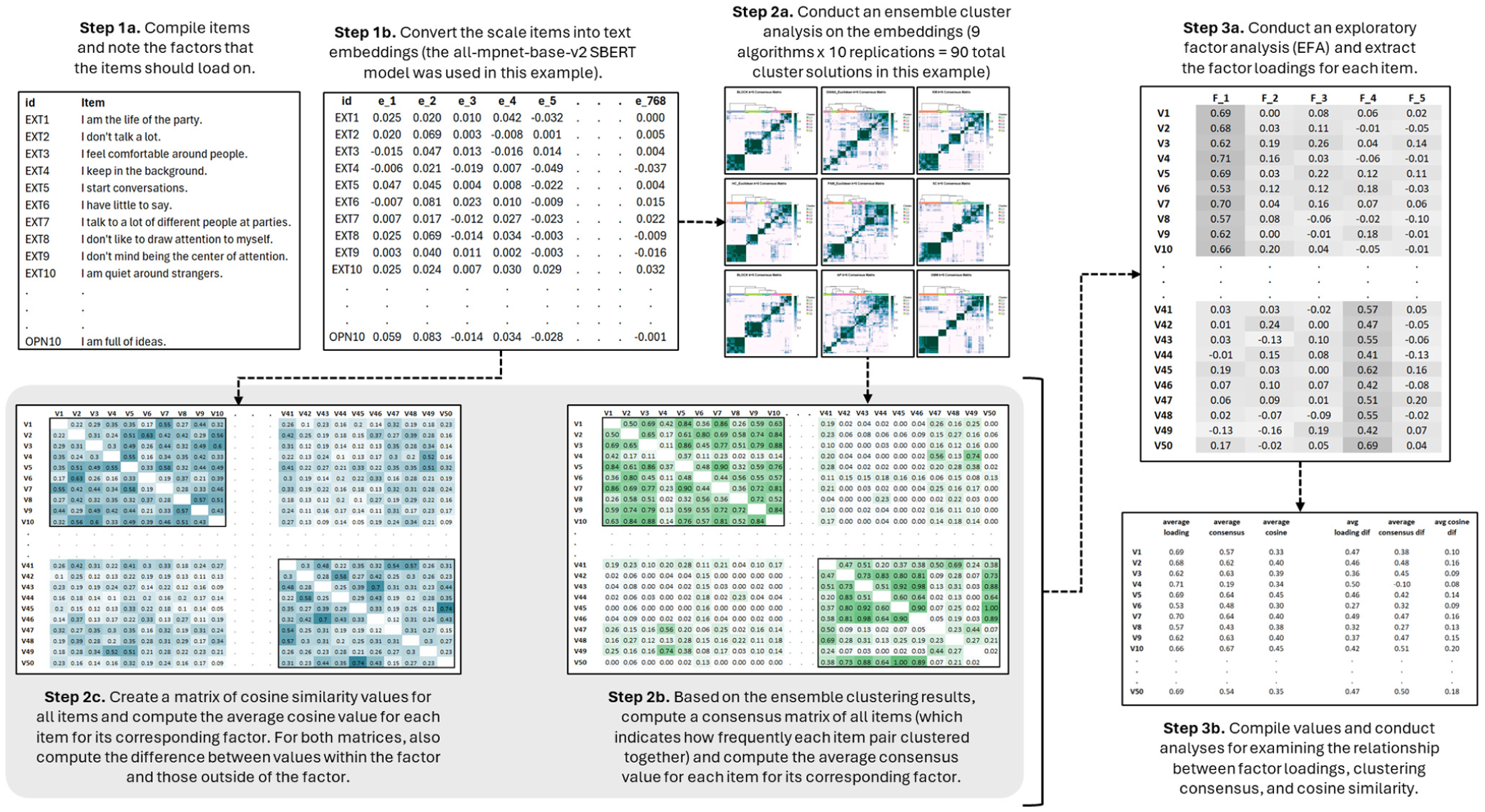
Summary of the workflow for using text embeddings, ensemble clustering, and cosine similarity to predict factor loadings.

Data Sources and Instruments

Response data for six self-report instruments were drawn from public sources. The Open-Source Psychometrics Project (Goldberg et al., 2006) provided the data for the first four instruments under a Creative Commons License, the U.S. Office of Personnel Management for the fifth, and the Open Science Framework for the last. No additional institutional review board approval was required for secondary analysis of these de-identified, publicly available data. Missing data were minimal across all scales (< 2% per item), and sample sizes exceeded 15,000 for all instruments. See Table 1 for a summary of sample sizes, item counts, factor counts, and data sources.

Table 1.

Summary of Scales Examined, Sample Sizes, Factor Numbers, and Item Numbers.

Scale	Sample size	Number of factors	Number of items
1. Big Five (IPIP Markers)	1,015,341	5	50
2. Dark Triad (Short)	18,192	3	27
3. HEXACO	22,786	6	240
4. RIASEC	145,828	6	48
5. Engagement (FEVS)	625,568	3	15
6. IPIP-300-NEO	307,313	5	300

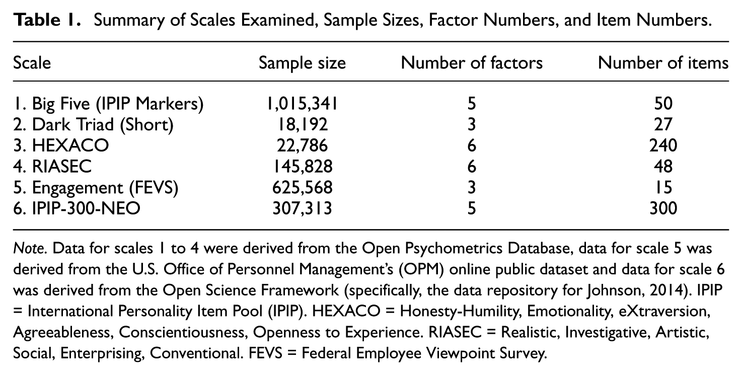
Note. Data for scales 1 to 4 were derived from the Open Psychometrics Database, data for scale 5 was derived from the U.S. Office of Personnel Management’s (OPM) online public dataset and data for scale 6 was derived from the Open Science Framework (specifically, the data repository for Johnson, 2014). IPIP = International Personality Item Pool (IPIP). HEXACO = Honesty-Humility, Emotionality, eXtraversion, Agreeableness, Conscientiousness, Openness to Experience. RIASEC = Realistic, Investigative, Artistic, Social, Enterprising, Conventional. FEVS = Federal Employee Viewpoint Survey.

International Item Personality Pool (IPIP) Big Five Factor Markers

The IPIP Big Five Markers (Goldberg, 1999) is a 50-item measure that assesses the Big Five personality traits (Extraversion [α = .89], Agreeableness [α = .83], Conscientiousness [α = .80], Neuroticism [α = .86], and Openness [α = .79]), with N = 1,015,341 respondents.

Dark Triad–Short

The Dark Triad–Short (Jones & Paulhus, 2014) includes 27 items measuring three factors (Machiavellianism [α = .86], Narcissism [α = .80], and Psychopathy [α = .80]) with N = 18,192 respondents.

HEXACO-60

The HEXACO-60 (Ashton et al., 2007) contains 240 items measuring six factors (Honesty-Humility [α = .90], Emotionality [α = .92], Extraversion [α = .95], Agreeableness [α = .94], Conscientiousness [α = .92], and Openness [α = .89]) with N = 22,786 respondents.

Interest Item Pool (IIP) RIASEC Markers

These RIASEC markers (Liao et al., 2008) include 48 items measuring six vocational interest factors (Realistic [α = .88], Investigative [α = .89], Artistic [α = .86], Social [α = .85], Enterprising [α = .84], and Conventional [α = .90]) with N = 145,828 respondents.

Federal Employee Viewpoint Survey (FEVS)

Employee Engagement data were drawn from the 2023 FEVS (U.S. Office of Personnel Management, 2023), a census of U.S. federal employees with approximately 625,568 respondents; we used the 15-item Engagement index, which contains three a priori factors: “Leaders Lead” (α = .93), “Supervisors” (α = .95), and “Intrinsic Work Experience” (α = .89).

IPIP-300-NEO

The IPIP-NEO-300 (Johnson, 2014) contains 300 items measuring five broad factors (Extraversion [α = .94], Agreeableness [α = .91], Conscientiousness [α = .94], Neuroticism [α = .95], and Openness [α = .90]) and 30 facets with N = 307,313 respondents.

Generate Text Embeddings

Once the scales were compiled, we next converted the item text into a format that can be used to compute cosine similarity and perform ensemble clustering. For the current study, we used the “all-mpnet-base-v2” SBERT model from the sentence-transformers package (v5.1.0; Reimers & Gurevych, 2019) in Python (v3.13.0; Python Software Foundation, 2025) for three reasons. First, this model achieves high performance across many benchmarks (Reimers & Gurevych, 2019). Second, it has demonstrated effectiveness in related psychometric applications, including item classifications (Hernandez & Nie, 2023), factor structure recovery (Milano, Luongo, et al., 2025), and clustering of psychological constructs (Hommel & Arslan, 2024). Third, it produces 768-dimensional dense embeddings suitable for both cosine similarity computation and clustering algorithms, enabling a unified representation for both text-derived signals.

The all-mpnet-base-v2 model also excels at semantic similarity tasks as it was specifically fine-tuned on a large corpus of 1 billion sentence pairs to produce high-quality dense vector representations that effectively capture semantic meaning. This is well-aligned with the current project, where we aimed to group semantically similar items together as a means for making potential inferences about factor loadings of those items. Each item stem was embedded as is without preprocessing such as lowercasing or punctuation removal, preserving semantic nuance that may contribute to construct meaning. For example, items phrased as questions (e.g., “Do you enjoy meeting new people?”) retained their question structure, and items with negation (e.g., “I do not seek attention”) retained the negation marker. Each item was embedded once, producing a fixed 768-dimensional vector used for all downstream analyses.

Compute Consensus and Cosine Matrices

After computing the embeddings, we constructed a (1) cosine similarity matrix and (2) an ensemble-based consensus matrix for each scale (see Figure 1). To produce the cosines for each scale, we applied the following formula for computing cosine similarity for each item pair until the full matrix was formed for each of the six scales:

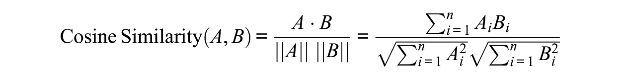
Cosine Similarity (A, B) = \frac{A \cdot B}{| | A | | | | B | |} = \frac{\sum_{i = 1}^{n} A_{i} B_{i}}{\sqrt{\sum_{i = 1}^{n} A_{i}^{2}} \sqrt{\sum_{i = 1}^{n} B_{i}^{2}}}

Here, n refers to the number of dimensions and i is the index of a dimension. A × B represents the dot product vectors of A and B, while ||A|| and ||B|| represent the magnitude (i.e., length) of vectors A and B, respectively. The numerator on the rightmost side represents the sum of element-wise products, while the denominator represents the product of the square roots of the sum of squares for each vector. As mentioned earlier, cosine similarity can range from −1 to +1, such that higher values indicate greater similarity.

To fully leverage the benefits of ensemble clustering, we employed a diverse set of clustering algorithms. Specifically, to perform ensemble clustering and compute the consensus matrix, we used the “dicer” package (v2.2.0; Chiu & Talhouk, 2018) in R (v4.3.0; R Core Team, 2024). For each scale, we employed the following nine distinct clustering algorithms (a discussion of the varying strengths and weaknesses of each algorithm is out of scope): (1) Hierarchical Clustering (with Ward linkage), (2) Divisive Analysis Clustering (DIANA), (3) k-Means Clustering, (4) Partition Around Medoids (PAM), (5) Affinity Propagation, (6) Spectral Clustering (normalized cuts), (7) Gaussian Mixture Modeling (GMM), (8) Latent Block Model Bi-Clustering, and (9) Self-Organizing Map (SOM). These algorithms were selected to span fundamentally different partitioning philosophies, including centroid-based methods (k-means, PAM), hierarchical methods (Ward, DIANA), density-based methods (affinity propagation), graph-based methods (spectral), model-based methods (GMM, latent block), and neural methods (SOM). This breadth ensures that consensus reflects agreement across diverse approaches rather than convergence within a single algorithmic family. Although there are other clustering algorithms supported by this package, we opted not to include them due to their complexity violating principles of parsimony or they were not appropriate for our focus on factor loadings. For logistical reasons, we also did not include algorithms such as non-negative matrix factorization (nmf) due to involving dependencies on third-party R packages not verified by the Comprehensive R Archive Network (CRAN). Nonetheless, we view the nine clustering algorithms we selected as sufficiently representative for illustrating the ensemble clustering approach, and expect that future research can continue to examine other algorithm combinations.

Moreover, to further ensure robust results, each clustering algorithm was run on random 80% subsamples¹ of items with 10 replications per algorithm, mitigating non-determinism and outlier influence. In total, 90 partitions were produced per scale (9 algorithms × 10 replications). The number of clusters was fixed to the number of factors for each scale (e.g., k = 5 for the IPIP Big Five Markers; k = 6 for HEXACO), which allowed us to explicitly explore the alignment between text-based groupings and subsequent factor loadings. The outcome of this step was a consensus matrix that records, for each item pair, the proportion (or percentage) of partitions in which the items appeared in the same cluster. Higher values indicate more frequent co-clustering by the ensemble. Across algorithms and resamples, we build a consensus matrix C, which recorded these proportions. Let Rij be the set of runs in which both items i and j were present (80% subsampling can omit one or both items), and let cluster r(·) denote the cluster label in run r. The co-assignment proportion is:

C_{ij} = \frac{1}{| R_{ij} |} \sum_{r \in R_{ij}} I ({cluster}_{r} (i) = {cluster}_{r} (j))

For item i intended for factor k with the same-factor set F_k, the consensus-within score averages co-assignment with its same-factor peers:

C W_{i} = \frac{1}{| F_{k} | - 1} \sum_{j \in F_{k} j \neq i} C_{ij}

Once the cosine similarity and consensus matrices were produced, we computed two sets of values to serve as predictors of factor loadings. First, we computed the average similarity of each item to other items within its intended factor (for both cosine and consensus). Let F_k denotes the set of items keyed to item i’s intended factor k, $F_{\neg k}$ its complement, and let $K_{ij} \in {\cos (i, j), C_{ij}}$ . The within summary and the within-outside contrast are:

\begin{matrix} K_{w} (i) = \frac{1}{| F_{k} | - 1} \sum_{j \in F_{k} j \neq i} K_{ij} \\ K_{wo} (i) = K_{w} (i) - \frac{1}{| F_{\neg k} |} \sum_{j \in F_{\neg k}} K_{ij} \end{matrix}

As an example, consider the Dark Triad—Short (see Figure 2), which contains 27 items, and 9 items per factor. For each item within a factor, one can compute the average consensus value of that item with the other items of the same underlying factor (called “Avg Within” in Figure 2, also denoted by the values shaded in dark gray). One can also compute the difference between these values and the consensus values of the item outside of its intended factor (called “Avg W-O [Within-Outside] Dif” in Figure 2, also denoted by the values in light gray). As noted above, this latter approach is useful in that it can better account for situations where values might be high both within and outside the intended factor (be it the consensus values, cosine values, or factor loadings), which is not desirable (since this would indicate an item is more similar to items in another factor, or a factor loading is cross-loading onto something other than its intended factor) and cannot be accounted for by only examining items within a given factor without reference to items outside of the factor. We used this same approach for computing the cosines and factor loadings (i.e., examining the average within-factor values and the within-factor/outside-factor difference values) across all six scales.

Figure 2.

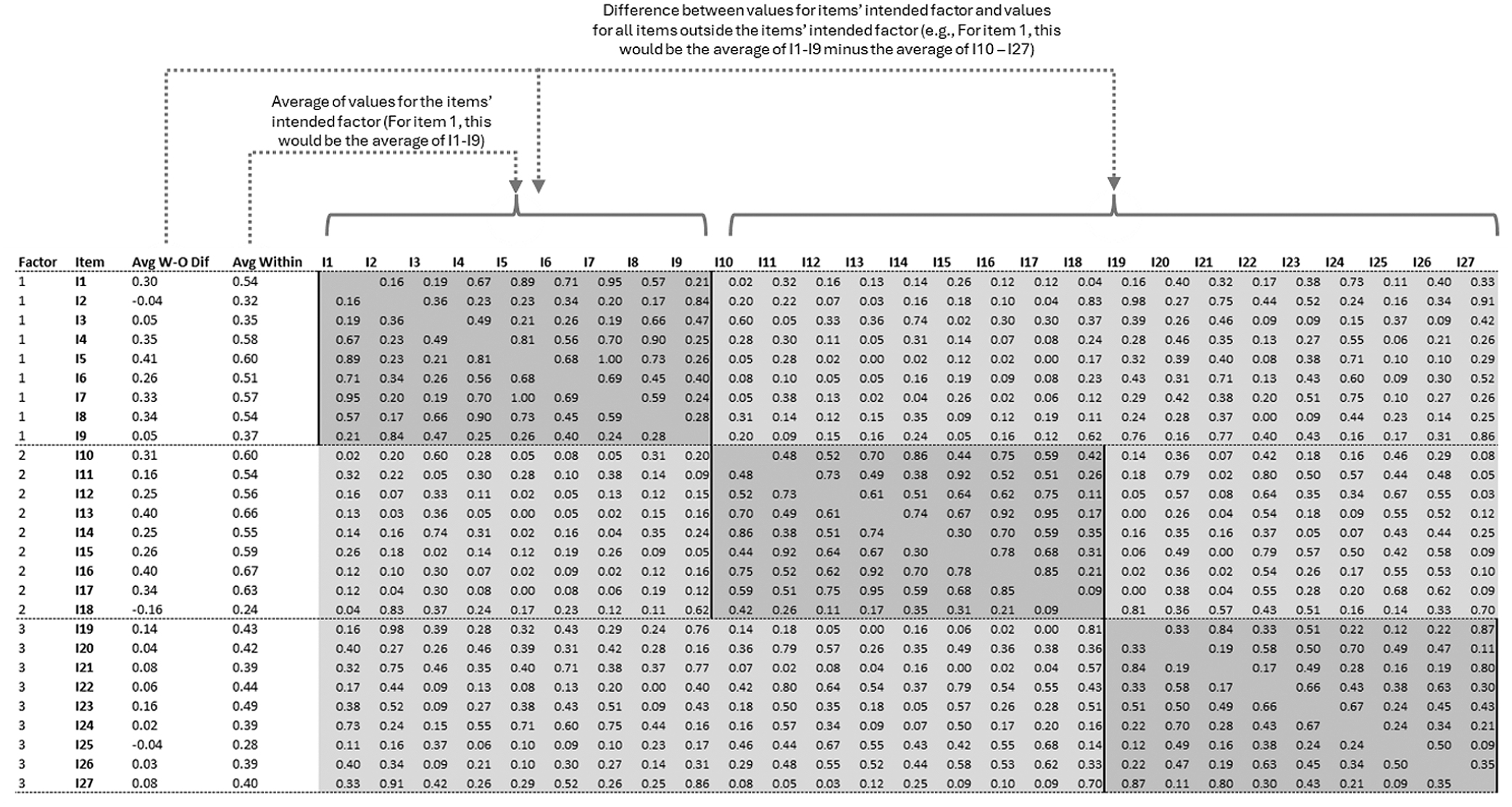
Example of how consensus values are computed across the consensus matrix for the Dark Triad—Short scale.

In total, we computed four predictors per item: cosine-within, cosine W-O, consensus-within, and consensus W-O. These predictors were computed separately for each scale and then added into a single dataset for regression analysis, along with a Scale identifier to enable the inclusion of interactions. Table 2 reports descriptive statistics for all four predictors by scale.

Table 2.

Descriptive Statistics for the Factor Loading, Clustering Consensus, and Cosine Similarity Metrics.

	Factor Loading		Clustering consensus		Cosine Similarity
Scale	M	SD	M	SD	M	SD
Average Within
1. Big Five (IPIP Markers)	.57	(.11)	.52	(.16)	.36	(.07)
2. Dark Triad (Short)	.49	(.12)	.48	(.12)	.28	(.05)
3. HEXACO	.44	(.14)	.30	(.09)	.29	(.07)
4. RIASEC	.63	(.11)	.67	(.20)	.27	(.09)
5. Engagement (FEVS)	.75	(.09)	.68	(.19)	.52	(.08)
6. IPIP-300-NEO	.41	(.14)	.29	(.08)	.28	(.07)
Average W-O Difference
1. Big Five (IPIP Markers)	.33	(.13)	.36	(.21)	.12	(.07)
2. Dark Triad (Short)	.18	(.16)	.20	(.16)	.08	(.06)
3. HEXACO	.19	(.13)	.12	(.10)	.07	(.05)
4. RIASEC	.39	(.14)	.59	(.23)	.18	(.09)
5. Engagement (FEVS)	.49	(.16)	.51	(.27)	.15	(.07)
6. IPIP-300-NEO	.16	(.12)	.08	(.10)	.05	(.04)

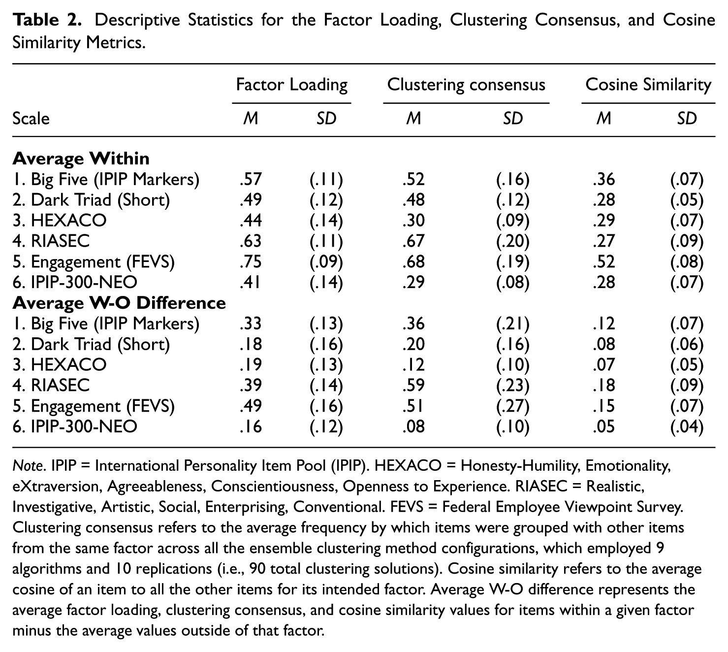
Note. IPIP = International Personality Item Pool (IPIP). HEXACO = Honesty-Humility, Emotionality, eXtraversion, Agreeableness, Conscientiousness, Openness to Experience. RIASEC = Realistic, Investigative, Artistic, Social, Enterprising, Conventional. FEVS = Federal Employee Viewpoint Survey. Clustering consensus refers to the average frequency by which items were grouped with other items from the same factor across all the ensemble clustering method configurations, which employed 9 algorithms and 10 replications (i.e., 90 total clustering solutions). Cosine similarity refers to the average cosine of an item to all the other items for its intended factor. Average W-O difference represents the average factor loading, clustering consensus, and cosine similarity values for items within a given factor minus the average values outside of that factor.

Compute Factor Loadings

As the final step, we computed the EFA factor loadings, which represent our key outcome of interest within the present study (Figure 1 Step 3a). This was accomplished using varimax rotation and maximum likelihood estimation as the factor extraction method for each scale examined. Factor loadings were extracted using the “fa” function in the “psych” package (v 2.4.3; Revelle, 2024). Varimax rotation was selected over oblique rotations (e.g., oblimin, promax) to produce an orthogonal factor structure to facilitate interpretability even when factors are moderately correlated. That said, we ran a separate robustness check to compare the varimax rotated factor loadings to the loadings estimated via oblimin rotation.² Generally, we found that correlations between varimax and oblimin loadings exceeded r = .93 for all six scales, confirming that the choice of rotation does not unduly impact results in a systematic way.

For scales with reverse-coded items, these were re-coded prior to computing the loadings such that higher values for all items indicated greater amounts of the measured construct. Similar to the consensus and cosine values, we examined the (1) factor loading values for their intended factor and (2) the difference between the factor loading values for an item’s intended factor and its average factor loading value for the remaining factors of the scale.

We evaluated two outcomes across items. The first, within-factor loading simply equals the value of the loading for a given item’s intended factor. The second, the loading-difference outcome, quantifies distinctiveness by contrasting the within-factor loading against the item’s loading on other factors. The within-outside loading difference was computed as:

λ_{i}^{2} - {\bar{(λ_{j}^{2})}}_{j \neq i}

where $λ_{i}$ is the loading of an item on its intended factor and $λ_{j}$ is its loadings on all other factors. Positive values indicate the item loads more strongly on its intended factor than on others (desirable), while values near zero or negative indicate cross-loading (undesirable). For example, an item with a target loading of .70 and an average loading of .20 on other factors indicates strong distinctiveness (i.e., a difference value of .50). In contrast, if an item has a loading of .50 for its intended factor, and an average loading of .40 for the other factors, this would indicate low distinctiveness (i.e., a difference value of .10). Table 2 reports descriptive statistics for both outcomes by scale.³

Analysis Approach

Our analyses are primarily focused on a series of nested models to assess the incremental validity of each set of predictors. Other than the four predictors described above, we also included Scale as an additional predictor. Scale was coded as a six-level categorical variable (Big Five, Dark Triad, HEXACO, RIASEC, FEVS, and IPIP-NEO-300) with Big Five as the reference level. All variables were standardized via z-scores, and continuous predictors were further mean-centered before computing interaction terms to reduce multicollinearity and aid interpretation of main effects. For within-factor outcomes, we estimated the following nested model sequence to test incremental validity:

Model 1: Within-factor loading regressed on consensus-within only.

Model 2: Add Scale and Scale-by-consensus-within interactions, testing whether consensus effects vary by measure.

Model 3: Within-factor loading regressed on cosine-within only (comparison with Model 1).

Model 4: Add consensus-within to Model 3, testing incremental variance of consensus beyond cosine.

Model 5: Add Scale main effects to Model 4, testing incremental validity of Scale beyond consensus and cosine.

Model 6: Add all Scale-by-cosine-within and Scale-by-consensus-within interactions.

For within-outside difference outcomes, we fitted similar models, but using the W-O predictors (i.e., cosine_dif and consensu_dif) instead of the within predictors.

Results

Descriptive Statistics

Before examining whether cosine similarity or item clustering consensus predicts factor loadings, we computed descriptive statistics (Mean [M], Standard Deviation [SD]) of each of the variables across all six scales (Table 2). Descriptives were examined for the average within-factor values (top part of Table 2) and difference values (bottom part of Table 2). Overall, the Engagement—FEVS scale had the highest factor loadings (M = .75, SD = .09), clustering consensus (M = .68, SD = .19), and cosine similarity (M = .52, SD = .08) values. This was followed by the RIASEC for the factor loadings (M = .63, SD = .11) and clustering consensus values (M = .67, SD = .20), though the Big Five IPIP Markers scale had the second highest cosine similarity value (M = .36, SD = .07). In contrast, the IPIP-300-NEO (Factor loading M = .41, SD = .14; Clustering consensus M = .29, SD = .08; Cosine similarity M = .28, SD = .07) and HEXACO (Factor loading M = .44, SD = .14; Clustering consensus M = .30, SD = .09; Cosine similarity M = .29, SD = .07) had the lowest values. A very similar pattern of results was observed for the average within-outside difference values, with the exception that these values tended to be lower overall (which is unsurprising since these are difference values). In general, values tended to be higher for scales with a smaller number of items (FEVS and RIASEC) but lower for scales with a large number of items (IPIP-NEO-300 and HEXACO).

Correlations Between Outcome and Methods

We next examined the correlations between the factor loadings, cosine similarity, and cluster consensus values (Table 3 and Figure 3). Figure 3 displays these associations as six-panel scatterplots, with each panel representing one scale for both cosine and consensus against factor loadings. For the within-factor values (top part of Table 3), the correlations between the cosines and factor loadings (Table 3, column 2) were slightly higher than the correlations between the clustering consensus values and factor loadings (Table 3, column 1). The Engagement—FEVS scale had the highest correlation between the factor loadings and cluster consensus (r = .51) and cosine (r = .88) values, whereas the RIASEC scale had the lowest correlation between the factor loadings and cluster consensus (r = .14) and cosine (r = .24) values.

Table 3.

Correlations Between the (1) Factor Loadings and Cluster Consensus Values, (2) Factor Loadings and Cosine Similarity Values, and (3) Cluster Consensus and Cosine Similarity Values.

Scale	Factor loading-cluster consensus r	Factor loading-cosine similarity r	Cluster consensus-cosine similarity r
Average Within Values
1. Big Five (IPIP Markers)	.29	.46	.51
2. Dark Triad (Short)	.34	.28	.50
3. HEXACO	.18	.28	.64
4. RIASEC	.14	.24	.77
5. Engagement (FEVS)	.51	.88	.68
6. IPIP-300-NEO	.28	.32	.56
Average W-O Difference Values
1. Big Five (IPIP Markers)	.28	.47	.78
2. Dark Triad (Short)	.46	.82	.43
3. HEXACO	.12	.28	.79
4. RIASEC	.18	.35	.80
5. Engagement (FEVS)	.40	.72	.84
6. IPIP-300-NEO	.23	.43	.77

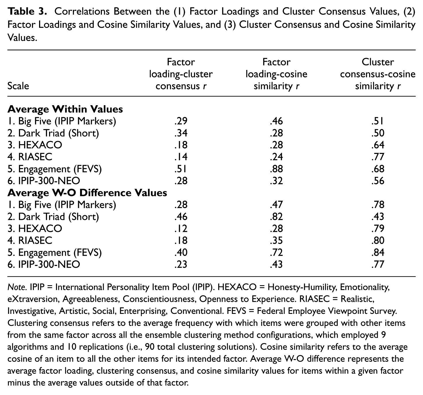
Note. IPIP = International Personality Item Pool (IPIP). HEXACO = Honesty-Humility, Emotionality, eXtraversion, Agreeableness, Conscientiousness, Openness to Experience. RIASEC = Realistic, Investigative, Artistic, Social, Enterprising, Conventional. FEVS = Federal Employee Viewpoint Survey. Clustering consensus refers to the average frequency with which items were grouped with other items from the same factor across all the ensemble clustering method configurations, which employed 9 algorithms and 10 replications (i.e., 90 total clustering solutions). Cosine similarity refers to the average cosine of an item to all the other items for its intended factor. Average W-O difference represents the average factor loading, clustering consensus, and cosine similarity values for items within a given factor minus the average values outside of that factor.

Figure 3.

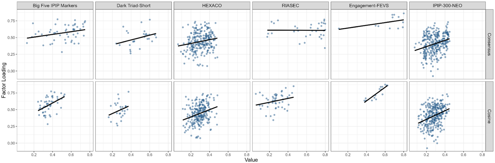
Visualization of the correlations between factor loadings and (1) cluster consensus and (2) cosine similarity.

In addition, across all scales, the clustering consensus and cosine similarity values were positively related, though these associations were not so high as to raise concerns that the two approaches are redundant (r range = .50 to .77; Table 3, column 3). A somewhat similar pattern of results was observed for the average within-outside factor values (bottom part of Table 3), though the rank order of the correlations slightly changed. Specifically, the Dark Triad—Short scale now had the highest correlation between the factor loading and clustering consensus (r = .46) and cosine (r = .82) values, while the HEXACO had the lowest correlation between the factor loading and clustering consensus (r = .12) and cosine (r = .28) values. When examining the difference values, the clustering consensus and cosine similarity methods were again positively related, with the relationships being slightly stronger on average compared with the previous analysis (r range = .43 to .84; Table 3, column 3).

Regression Models Predicting Factor Loadings

We next estimated a series of regression models to determine how much variance in the factor loading values can be accounted for by clustering consensus and cosine similarity. This was accomplished by including all scale items and relevant variables (e.g., factor loadings, cosine similarity, and clustering consensus values) into a single file for analysis (total items = 680). This was done to enable direct statistical comparison of scale-level effects through interaction terms and to address the instability that would arise from fitting separate models to small-item scales. For example, Engagement–FEVS has only 15 items and Dark Triad–Short has 27, yielding fewer than 30 observations per parameter if scale-specific interactions were estimated within-scale, which would produce unreliable coefficients and inflated standard errors.

The regression results indicated that Model 1 could explain a significant amount of the variance in factor loadings (R² = .24, F(1, 678) = 211.48, p < .001, upper part of Table 4). Adding the Scale, along with all scale-by-consensus interactions as predictors in Model 2, increased the total R² to .30, F(11, 668) = 25.86, p < .001.

Table 4.

Summary of the Regression Models Predicting Factor Loadings Via Clustering Consensus and Cosine Similarity.

Predictor	R ²	ΔR²	Model F	p-value
Average Within Values
Consensus Only
1. Model 1: Consensus	.24	—	211.48	<.001
2. Model 2: Consensus + Scale + Interaction	.30	.06	25.86	<.001
Cosines + Consensus
3. Model 3: Cosines	.15	—	120.14	<.001
4. Model 4: Cosines + Consensus	.26	.11	121.68	<.001
5. Model 5: Cosines + Consensus + Scale	.32	.06	46.73	<.001
6. Model 6: Cosines + Consensus + Scale + Interaction	.34	.02	19.79	<.001
Average W-O Difference Values
Consensus Only
1. Model 1: Consensus	.25	—	226.73	<.001
2. Model 2: Consensus + Scale + Interaction	.32	.07	28.09	<.001
Cosines + Consensus
3. Model 3: Cosines	.31	—	300.24	<.001
4. Model 4: Cosines + Consensus	.31	.00	152.03	<.001
5. Model 5: Cosines + Consensus + Scale	.39	.08	61.68	<.001
6. Model 6: Cosines + Consensus + Scale + Interaction	.41	.02	27.23	<.001

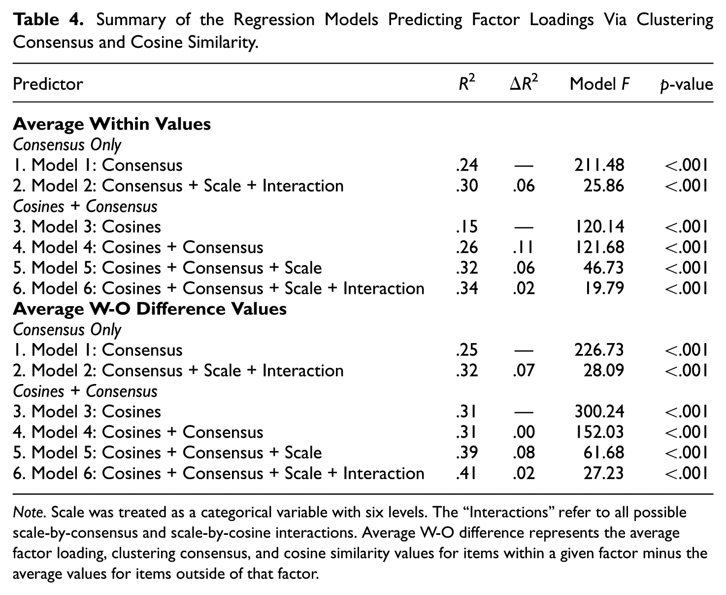
Note. Scale was treated as a categorical variable with six levels. The “Interactions” refer to all possible scale-by-consensus and scale-by-cosine interactions. Average W-O difference represents the average factor loading, clustering consensus, and cosine similarity values for items within a given factor minus the average values for items outside of that factor.

When examining only cosine similarity as a predictor, Model 3 was again significant, R² = .15, F(1, 678) = 120.14, p < .001, though the R² compared with Model 1 was slightly lower. Adding the clustering consensus values in Model 4 explained incremental variance, total R² = .26, F(2, 677) = 121.68, p < .001. Moreover, adding the Scale main effects to Model 4 in Model 5, also showed incremental variance, total R² = .33, F(7, 672) = 46.73, p < .001. Finally, adding all scale-by-cosine and scale-by-consensus interactions as predictors in Model 6 yielded a model with an R² of .34, F(17, 662) = 19.79, p < .001. Except for the Models 5 to 6 comparison, each nested model comparison was statistically significant (see Table 5). These results suggest that (1) clustering consensus predicts incremental variance above and beyond cosine similarity and (2) it is important to account for how the effects of cosine similarity and clustering consensus vary across different scales (see also Figure 3 and Table 3).

Table 5.

Regression Model Comparisons.

Comparison	df1	df2	Model F	p-value
Average Within Values
Consensus Only
Model 1 vs Model 2	10	668	5.80	<.001
Cosines + Consensus
Model 3 vs Model 4	1	677	113.73	<.001
Model 4 vs Model 5	5	672	12.57	<.001
Model 5 vs Model 6	10	662	0.96	.48
Average W-O Difference Values
Consensus Only
Model 1 vs Model 2	10	668	6.42	<.001
Cosines + Consensus
Model 3 vs Model 4	1	677	3.38	.07
Model 4 vs Model 5	5	672	18.28	<.001
Model 5 vs Model 6	10	662	2.29	.01

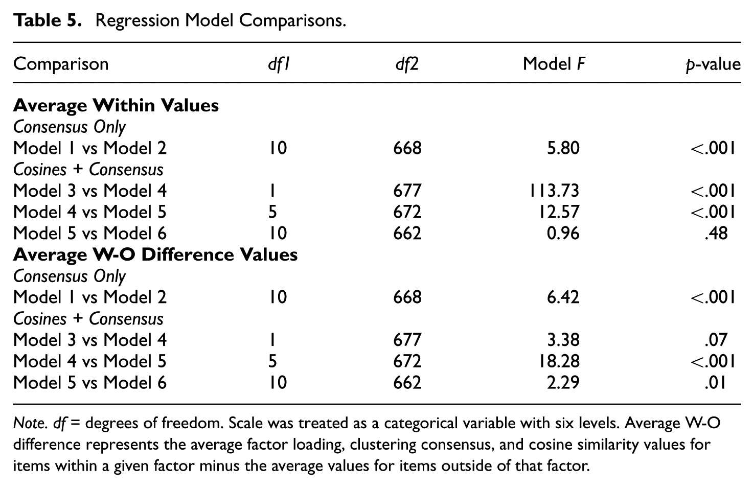
Note. df = degrees of freedom. Scale was treated as a categorical variable with six levels. Average W-O difference represents the average factor loading, clustering consensus, and cosine similarity values for items within a given factor minus the average values for items outside of that factor.

Regression Models Predicting Factor Loadings Within-Outside Differences

We next estimated a series of regression models with the various difference values as the predictors and outcomes. The results again indicated that Model 1, containing only the consensus_dif values, was a significant predictor of factor loadings_dif (R² = .25, F(1, 678) = 226.73, p < .001, lower part of Table 4). Adding Scale, and all scale-by-consensus_dif interactions (again all centered) in Model 2 increased the R² to .32, F(11, 668) = 28.09, p < .001. When examining the cosine similarity_dif as the sole predictor, Model 3 was also significant (R² = .31, F(1, 678) = 300.24, p < .001). Adding the consensus_dif values to this model in Model 4 did not increase the R², which remained .31, F(2, 677) = 152.03, p < .001, and did not represent a statistically significant increase from Model 3 (see Table 5). Adding Scale in Model 5, however, increased R² to .39, F(7, 672) = 61.68, p < .001. Moreover, adding all scale-by-consensus_dif and scale-by-cosine_dif interactions for Model 6 also increased R² to .41, F(17, 662) = 27.23, p < .001. All model comparisons were statistically significant, barring the Models 3 and 4 comparison (see Table 5). Again, these results affirm the importance of the Scale when using either the cosine_dif or clustering consensus_dif methods to predict factor loadings_dif.

Discussion

The primary objective of this study was to examine how recent advances in NLP and LLMs (i.e., text embeddings) could be used to evaluate the psychometric properties of scale items prior to data collection. We sought to determine if a novel application of ensemble clustering within a psychometrics context, in addition to a cosine similarity-based method, could predict item factor loadings. Our findings provide supportive answers to our research questions and demonstrate the value of NLP approaches in the early stages of scale development.

With regard to Research Question 1, we found that both the ensemble clustering consensus and the cosine similarity methods were effective in predicting EFA factor loadings based on text alone. That is, items that were more frequently grouped with other items from the same underlying factor (clustering consensus) and items that were more semantically similar to their intended-factor counterparts (cosine similarity) tended to have higher factor loadings. This core finding aligns with and extends previous research that has successfully used embedding-based techniques to predict other psychometric features (e.g., Feraco & Toffalini, 2025; Milano, Luongo, et al., 2025), such as interitem correlations and overall factor structures.

A key contribution of our study, and an answer to Research Question 2, is the finding that the ensemble clustering approach explains incremental variance in factor loadings above and beyond what is explained by cosine similarity alone. While the two methods are conceptually related—both being derived from text embeddings—and empirically correlated, the magnitude of the correlation between methods suggested they were not redundant. This supports the notion that they capture different aspects of item relationships. This finding was particularly evident in the primary analysis of average within-factor values. Interestingly, when using the more refined “difference” scores—which control for an item’s general similarity to all other items—the predictive power of cosine similarity increased substantially, suggesting it is highly effective at capturing an item’s unique semantic contribution to its factor. This provides some initial evidence of a potential semantic analog to examining discriminant validity at the item level. Nonetheless, the full model including scale interactions was still superior, reaffirming that using both approaches to evaluate items is optimal, though this differs across different scales.

The superiority of the ensemble clustering approach may stem from its more holistic assessment; it considers all items jointly to form groups, which is more analogous to how factor loadings are computed in an EFA. In contrast, cosine similarity relies on a series of simple, pairwise comparisons, which may not capture the more nuanced, systemic patterns of association among a full set of scale items. Whereas cosine similarity provides a series of independent, pairwise local comparisons, ensemble clustering offers a global solution by partitioning the entire set of items simultaneously. This process inherently accounts for the complex, higher-order relationships within the entire semantic space of the scale, rather than just the direct similarity between two items. Further, based on Ghosh and Acharya (2011), we reason that the ensemble method’s use of multiple clustering algorithms likely averages out the idiosyncratic biases of any single clustering approach, resulting in a more stable and robust signal of item congruence.

In addressing Research Question 3, we found that the predictive utility of both methods varied notably across the six different scales examined. The inclusion of the “Scale” variable and its interactions substantially improved the regression models, indicating that characteristics unique to each scale—such as the number of items, the number of factors, or the nature of the construct being measured—influence the relationship between semantic features and factor loadings. Although the current study did not reveal an obvious pattern explaining these differences, this finding underscores the importance of context and suggests that a one-size-fits-all approach may not be optimal. This also suggests a useful avenue for future research to explore in greater detail. For example, one potential explanation relates to scale breadth and item density. The methods appeared to perform best on scales with fewer items (e.g., Engagement-FEVS). It is plausible that on large, broad-bandwidth measures like the IPIP-300-NEO, the semantic space is far more crowded, making it more difficult for algorithms to discern clear clusters. Conversely, shorter, more focused scales may present a cleaner semantic signal.

Practical Implications

The findings from this study offer a valuable and practical workflow for researchers engaged in scale development. Before committing resources to large-scale data collection, developers can employ this two-pronged analytic approach as an empirical “prescreening” tool. A simple workflow could involve: (1) generating embeddings for a new item pool; (2) calculating both the cosine similarity and ensemble clustering consensus for each item relative to its intended factor; and (3) flagging items that exhibit both low similarity and low consensus. Such items can be identified as potentially problematic and subsequently revised or removed, thereby potentially enabling more successful item pilot testing.

A crucial consideration when implementing this workflow is the notable variability in predictive effects observed across different instruments. This suggests that while these methods are powerful for identifying the relative strength of items within a single developing scale, researchers should be cautious about applying absolute cutoff values derived from one scale to another. Therefore, the primary utility of this prescreening tool lies in its ability to rank-order and triage candidate items for a specific measure, rather than establishing universal benchmarks for item quality. We also note that this methodology is not intended to replace traditional validation procedures like expert content reviews, EFA, or CFA. Rather, it serves as a powerful, data-driven supplement to the initial item-writing and refinement stages. By helping to weed out semantically incongruous or ambiguous items from the onset, this approach can significantly increase the efficiency of the scale development process and improve the likelihood of a successful validation study, thus saving invaluable time and resources.

Item Retention/Removal Decision-Making Framework

To further illustrate the practical value of this method, we present a framework (see Figure 4) for supporting item prescreening decisions (e.g., whether to retain, further review, or drop items). When jointly considering the consensus and cosine metrics, four scenarios are possible: (Scenario 1) high consensus/high cosine (Figure 4, top left), (Scenario 2) high consensus/low cosine (Figure 4, bottom left), (Scenario 3) low consensus/high cosine (Figure 4, top right), and (Scenario 4) low consensus/low cosine (Figure 4, bottom right). In this framework, the ideal items to retain are those with high consensus and high cosine values, as these are the items most likely to have high factor loadings (note this is also corroborated by the finding that clustering consensus values explains incremental variance in predicting factor loadings above and beyond just cosine values). Furthermore, items with a high value for only either the consensus or cosine metrics represent edge cases that could potentially benefit from further review. Items with low consensus and cosine values, however, are least likely to have high factor loadings and could be considered good candidate items to drop. As a concrete example, consider some values that were derived for select items from the IPIP Big Five Markers within this study. The item “I get upset easily” had a consensus and cosine value of .74 and .53, respectively, and represents an ideal item (i.e., high consensus/high cosine). In contrast, the items “I am always prepared” (consensus = .62, cosine = .24; high consensus/low cosine) and “I take time out for others” (consensus = .22, cosine = .34; low consensus/high cosine) could benefit from further review since values were high on only one of the metrics. For the item, “I spend time reflecting on things,” both the consensus (.12) and cosine (.26) values were low, and thus this item represents a good candidate for removal.

Figure 4.

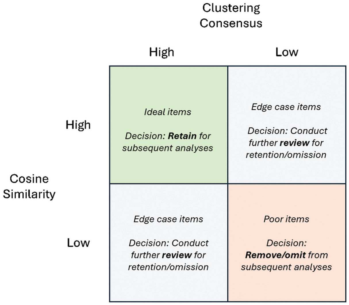
Decision framework and possible scenarios that may be encountered when prescreening items using consensus and cosine values.

Importantly, the goal of this framework is to provide a starting point for those interested in making categorial decisions (i.e., concerning item retention/removal) on the basis of the proposed method. Our goal is not necessarily to provide universal cutoffs or decision-making criteria for what constitutes a high or low consensus/cosine value, as this is likely going to depend on the nature of the scale, such as the magnitude and distribution of values, along with other scale-specific features. Indeed, the variability we observed across scales suggests that universal decision criteria may not be appropriate. Moreover, specific cutoffs will also likely depend on the researcher’s scale development goals, such as how many items they wish to retain/remove, how many items are developed for inclusion in the initial item pool, and how critical it is to ensure the scale contains items with high factor loadings. With that said, we believe this framework can help support different decision strategies. For instance, one could experiment with different absolute cutoffs to identify problematic items (e.g., consensus values less than .10, .20, .30, etc.) or explore problematic items using relative metrics (e.g., the lowest 10%, 20%, 30%, etc., consensus values). To illustrate this, Figure 5 shows the distribution of the cosine and consensus values for the six scales we explored in this study, with the bottom 10% of values being flagged (as black points) as items for potential review. This is just one such example, as other thresholds (absolute or relative) could be explored. One could also incorporate detection accuracy metrics and observe Type I/Type II errors at different thresholds (if ground truth was known/available) to further investigate what items should be retained/dropped. Examining items in this manner will allow one to derive various consensus/cosine configurations for each item (i.e., Figure 4) and therefore provides a flexible method for reviewing potentially problematic items and making initial retention/omission decisions.

Figure 5.

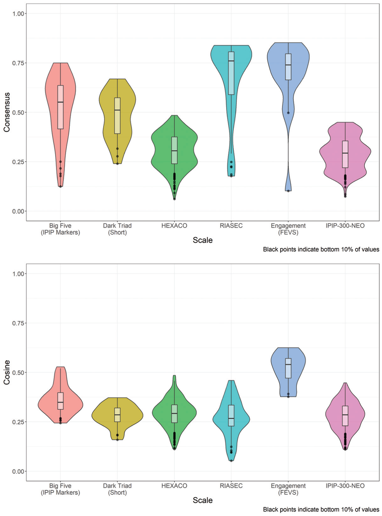
Violin plots depicting the distribution of consensus and cosine values and how items with low values can be flagged for further review.

Limitations and Future Directions

This study has several limitations that also point toward avenues for future research. First, our evaluation was conducted exclusively on established scales with hypothesized factor structures. For such instruments, items with poor psychometric properties have likely already been filtered out, creating the potential for range restriction in our outcome variables (i.e., factor loadings). Consequently, the predictive effects reported in this study likely represent a conservative estimate of the methods’ true utility, and could also suggest why some of the effects we observed were smaller. The fact that our models explained substantial variance even within this restricted context suggests their performance on a new, unvetted item pool—containing a wider range of item quality from poor to excellent—could be even more pronounced. Future research could explore this by applying these methods to a live scale development project, tracking predictions from the initial item pool through final validation.

Second, although we demonstrated that predictive effects vary across scales, we did not systematically investigate which scale characteristics (e.g., item length, construct abstractness, and number of items) might be responsible for such differences. Future research should investigate these potential moderators to build a more comprehensive understanding of when and why these methods are most effective. Third, our study used a single, high-performing sentence transformer model. The field of large language models is rapidly evolving, and future studies could compare the efficacy of different embedding models.

Finally, this research focused on predicting EFA factor loadings. An important next step would be to examine whether these methods can also predict confirmatory psychometric indicators, such as CFA factor loadings, model fit indices, or item discrimination parameters (e.g., Feraco & Toffalini, 2025). For example, given that ensemble clustering provides a global assessment of item fit within a factor, we expect that an item’s clustering consensus value may be a particularly strong predictor of its standardized loading in a subsequent CFA. Similarly, though standard CFA models constrain cross-loadings to zero, our text-based “difference score” could still be a powerful diagnostic tool; items with high within-factor similarity but also high between-factor similarity (i.e., a low difference score) could be proactively flagged as potential sources of localized model misfit or indicators of high modification indices in a CFA.

Conclusion

To help address the time-consuming and resource-intensive nature of traditional scale development, this study demonstrates that combining text embeddings with ensemble clustering and cosine similarity metrics can be a useful method for evaluating items prior to data collection. The novel application of ensemble clustering offers unique predictive utility beyond more traditional semantic similarity metrics. Although the effectiveness of these methods may vary across different measurement instruments, their use in conjunction offers a promising new method for the modern scale developer. By identifying and refining items at the earliest stage before data is gathered, this approach has the potential to save significant time and resources, ultimately increasing the likelihood of developing reliable and valid measures.

Footnotes

Declaration of Conflicting Interests

The authors declared no potential conflicts of interest with respect to the research, authorship, and/or publication of this article.

Funding

The authors received no financial support for the research, authorship, and/or publication of this article.

ORCID iD

Nathaniel M. Voss

Notes

References

Anvari

Alsalti

Oehler

L. A.

Marion

Hussey

Elson

Arslan

R. C.

(2025). A fragmented field: Construct and measure proliferation in psychology. Advances in Methods and Practices in Psychological Science, 8(3), 25152459251360642.

Ashton

M. C.

Lee

Goldberg

L. R.

(2007). The IPIP–HEXACO scales: An alternative, public-domain measure of the personality constructs in the HEXACO model. Personality and Individual Differences, 42, 1515–1526. https://doi.org/10.1016/j.paid.2006.10.027

Chiu

D. S.

Talhouk

(2018). DiceR: An R package for class discovery using an ensemble driven approach. BMC Bioinformatics, 19, 1–4.

Church

A. T.

Burke

P. J.

(1994). Exploratory and confirmatory tests of the Big Five and Tellegen’s three- and four-dimensional models. Journal of Personality and Social Psychology, 66(1), 93–114. https://doi.org/10.1037/0022-3514.66.1.93

DeVellis

R. F.

Thorpe

C. T.

(2021). Scale development: Theory and applications (5th ed.). Sage.

Devlin

Chang

M.-W.

Lee

Toutanova

(2019). BERT: Pre-training of deep bidirectional transformers for language understanding. Proceedings of NAACL-HLT, 2019, 4171–4186. https://arxiv.org/abs/1810.04805

Eberhardt

S. T.

Vehlen

Schaffrath

Schwartz

Baur

Schiller

Hallmen

André

Lutz

(2025). Development and validation of large language model rating scales for automatically transcribed psychological therapy sessions. Scientific Reports, 15, 29541. https://doi.org/10.1038/s41598-025-14923-y

Feraco

Toffalini

(2025). SEMbeddings: How to evaluate model misfit before data collection using large-language models. Frontiers in Psychology, 15, Article 1433339.

Flake

J. K.

Pek

Hehman

(2017). Construct validation in social and personality research: Current practice and recommendations. Social Psychological and Personality Science, 8(4), 370–378. https://doi.org/10.1177/1948550617693063

10.

Gao

C. X.

Wang

Zhu

Ziou

Teo

S. M.

Smith

C. L.

Chiu

Talhouk

Cotton

S. M.

Dwyer

(2024). Ensemble clustering: A practical tutorial. https://osf.io/preprints/psyarxiv/fq6e9_v1

11.

Ghosh

Acharya

(2011). Cluster ensembles. Wiley Interdisciplinary Reviews: Data Mining and Knowledge Discovery, 1(4), 305–315.

12.

Goldberg

L. R.

(1999). A broad-bandwidth, public domain, personality inventory measuring the lower-level facets of several five-factor models. Personality Psychology in Europe, 7(1), 7–28.

13.

Goldberg

L. R.

Johnson

J. A.

Eber

H. W.

Hogan

Ashton

M. C.

Cloninger

C. R.

Gough

H. G.

(2006). The international personality item pool and the future of public-domain personality measures. Journal of Research in Personality, 40(1), 84–96. https://doi.org/10.1016/j.jrp.2005.08.007

14.

Guenole

D’Urso

E. D.

Samo

Sun

(2024). Pseudo factor analysis of language embedding similarity matrices: New ways to model latent constructs. https://osf.io/preprints/psyarxiv/vf3se_v2

15.

Harber

J. G.

Day

E. A.

(2023, August 16). ASVAB item development process [Presentation]. Defense Advisory Committee on Military Personnel Testing. https://dacmpt.com/wp-content/uploads/2023/07/04-Item-Development-Process-Presentation-to-the-DACMPT-8-16-23-Read-Only.pdf

16.

Hennig

(2015). What are the true clusters? Pattern Recognition Letters, 64, 53–62.

17.

Hernandez

Nie

(2023). The AI-IP: Minimizing the guesswork of personality scale item development through artificial intelligence. Personnel Psychology, 76(4), 1011–1035.

18.

Hommel

B. E.

Arslan

R. C.

(2024). Language models accurately infer correlations between psychological items and scales from text alone. PsyArXiv. https://doi.org/10.31234/osf.io/kjuce

19.

James

Witten

Hastie

Tibshirani

(2013). An introduction to statistical learning. Springer.

20.

Johnson

J. A.

(2014). Measuring thirty facets of the Five Factor Model with a 120-item public domain inventory: Development of the IPIP-NEO-120. Journal of Research in Personality, 51, 78–89.

21.

Jones

D. N.

Paulhus

D. L.

(2014). Introducing the short dark triad (SD3) a brief measure of dark personality traits. Assessment, 21(1), 28–41.

22.

Kilmen

Bulut

(2025). Shortening psychological scales: Semantic similarity matters. Educational and Psychological Measurement, 85, 910–934.

23.

Lambert

L. S.

Newman

D. A.

(2023). Construct development and validation in three practical steps: Recommendations for reviewers, editors, and authors. Organizational Research Methods, 26(4), 779–809. https://doi.org/10.1177/10944281221115374

24.

Liao

H.-Y.

Armstrong

P. I.

Rounds

(2008). Development and initial validation of public domain Basic Interest Markers. Journal of Vocational Behavior, 73(1), 159–183. https://doi.org/10.1016/j.jvb.2007.12.002

25.

Maeda

(2025). Field-testing multiple-choice questions with AI examinees: English grammar items. Educational and Psychological Measurement, 85(2), 221–244. https://doi.org/10.1177/00131644241281053

26.

Marsh

H. W.

Lüdtke

Muthén

Asparouhov

Morin

A. J. S.

Trautwein

Nagengast

(2010). A new look at the Big Five factor structure through exploratory structural equation modeling. Psychological Assessment, 22(3), 471–491. https://doi.org/10.1037/a0019227

27.

Marsh

H. W.

Morin

A. J.

Parker

P. D.

Kaur

(2014). Exploratory structural equation modeling: An integration of the best features of EFA and CFA. Annual Review of Clinical Psychology, 10(1), 85–110. https://doi.org/10.1146/annurev-clinpsy-032813-153700

28.

McElroy

Wood

Bond

Mulvenna

Shevlin

Ploubidis

G. B.

Hoffmann

M. S.

Moltrecht

(2024). Using natural language processing to facilitate the harmonisation of mental health questionnaires: A validation study using real-world data. BMC Psychiatry, 24, 530. https://doi.org/10.1186/s12888-024-05954-2

29.

Mehta

Bawa

Singh

(2021). WEClustering: Word embeddings based text clustering technique for large datasets. Complex & Intelligent Systems, 7(6), 3211–3224.

30.

Milano

Luongo

Ponticorvo

Marocco

(2025). Semantic analysis of test items through Large Language Model embeddings predicts a-priori factorial structure of personality tests. Current Research in Behavioral Sciences, 8, 100168.

31.

Milano

Ponticorvo

Marocco

(2025). Human expertise and large language model embeddings in the content validity assessment of personality tests. Educational and Psychological Measurement, 86(1), 30–53.

32.

Monti

Tamayo

Mesirov

Golub

(2003). Consensus clustering: A resampling- based method for class discovery and visualization of gene expression microarray data. Machine Learning, 52, 91–118.

33.

Petukhova

Matos-Carvalho

J. P.

Fachada

(2025). Text clustering with large language model embeddings. International Journal of Cognitive Computing in Engineering, 6, 100–108.

34.

Python Software Foundation. (2025). Python language reference. https://www.python.org/

35.

R Core Team. (2024). R: A language and environment for statistical computing. R Foundation for Statistical Computing. https://www.R-project.org/

36.

Reeder

M. C.

(2023, August 16). ASVAB item development process: Item analysis [Presentation]. Defense Advisory Committee on Military Personnel Testing. https://dacmpt.com/wp-content/uploads/2023/07/05-Item_Analysis_Presentation-to-the-DACMPT-8-16-23-002-Read-Only.pdf

37.

Reimers

Gurevych

(2019). Sentence-bert: Sentence embeddings using siamese bert-networks. arXiv:1908.10084.

38.

Revelle

(2024). psych: Procedures for psychological, psychometric, and personality research. Northwestern University. https://CRAN.R-project.org/package=psych

39.

Soto

C. J.

John

O. P.

(2017). Short and extra-short forms of the Big Five Inventory–2 (BFI-2-S and BFI-2-XS): Reliable and efficient assessment of the Big Five domains and facets. Journal of Research in Personality, 68, 69–81. https://doi.org/10.1016/j.jrp.2017.02.004

40.

Stanton

Ramnarine-Rieks

Sang

(2024). Evaluating item content and scale characteristics using a pretrained neural network model. Survey Research Methods, 18(2), 153–165.

41.

Tay

Liao

H.-Y.

Zhang

Rounds

(2019). Toward a dimensional model of vocational interests. Journal of Applied Psychology, 104(5), 690–714. https://doi.org/10.1037/apl0000373

42.

U.S. Department of Defense. (2024). ASVAB fact sheet: Understanding the armed services vocational aptitude battery. https://www.officialasvab.com/wp-content/uploads/2024/02/ASVAB-Fact_Sheet.pdf

43.

U.S. Department of Defense. (2025). Official ASVAB website. https://www.officialasvab.com/

44.

U.S. Office of Personnel Management. (2023). Federal Employee Viewpoint Survey results: Technical report. https://www.opm.gov/fevs/reports/governmentwide-reports/governmentwide-reports/governmentwide-management-report/2023/2023-governmentwide-management-report.pdf

45.

Wendler

Bridgeman

(Eds.). (2014). The research foundation for the GRE® revised general test: A compendium of studies. Educational Testing Service.

46.

Wulff

D. U.

Mata

(2025). Semantic embeddings reveal and address taxonomic incommensurability in psychological measurement. Nature Human Behaviour, 9(5), 944–954.