Evaluating Factor Retention in Large Factor Analysis Models: A Simulation Study Comparing 15 Methods

Introduction

Exploratory factor analysis (EFA) is a crucial tool in behavioral research, commonly used for the development of new measurement instruments and for identifying latent constructs underlying observed variables. Over 75% of researchers involved in scale development incorporated EFA into their work (Conway & Huffcutt, 2003). Browne (2001) stated that conducting EFA before confirmatory factor analysis offers several advantages, including improved construct validity, clearer factor structures, and more informed model specification. In this sense, EFA is used primarily as an initial dimensionality-assessment step that helps narrow the set of plausible models for subsequent confirmatory factor analysis.

However, despite the important use of EFA, determining the appropriate number of factors remains a debated and challenging issue. Two common problems associated with factor retention are overfactoring and underfactoring. Underfactoring leads to loss of true variance explained (Fava & Velicer, 1996) and inadequate representation of indicator cross-loadings, making theoretical interpretation difficult for researchers (Wood et al., 1996). On the other hand, overfactoring is also problematic, as it can result in unnecessarily low factor loadings and confusing factor interpretation (e.g., Goretzko, 2025).

In previous research, many scholars have done simulation studies to evaluate different factor retention methods in different conditions. Nevertheless, previous simulation studies mainly generated data based on small to moderate EFA models (Auerswald & Moshagen, 2019; H. Golino et al., 2020). In contemporary psychological research, large factor models such as the Big Five model of personality (Hendriks et al., 1999) are widely used. These models often involve complex factor structures with more than five factors and 120 indicators (Saucier, 2009). In such cases, the number of retained factors can vary considerably depending on the retention method employed, which can have serious implications for the resulting theoretical framework (Lorenzo-Seva et al., 2011; Thalmayer et al., 2011).

In this study, large factor models refer to EFA structures with relatively more latent factors and indicators per factor, compared with those typically examined in prior simulation studies. Model size is therefore not treated as a vague or purely parameter-based concept. Instead, structural complexity is defined by two separate features: the number of latent factors and the number of indicators per factor. This definition is consistent with prior reviews of applied EFA research. Henson and Roberts (2006), for example, showed that empirical EFA applications commonly involve one to seven factors, whereas Howard (2023) documented applied studies in which factors were measured by relatively large numbers of indicators. Accordingly, this study defines comparatively large factor models using both dimensions rather than treating model size as a single undifferentiated characteristic.

Importantly, our use of the term large is grounded in an applied-research perspective rather than in the most extreme computational or theoretical definition of dimensional complexity. We do not claim that the present design represents the most difficult possible condition in the factor-retention literature. Rather, our objective is to evaluate factor retention methods’ performance under multidimensional structures that are realistic for applied EFA research, where researchers may encounter six or seven factors together with 10 to 15 indicators per factor. From this perspective, the goal of the study is not to maximize difficulty, but to provide evidence that is informative for applied researchers working with comparatively large multidimensional structures.

Prior simulation studies evaluated factor retention methods under a variety of conditions. However, their evaluations have rarely extended to large factor models. Two key questions emerge from prior evaluations of factor retention methods based on small factor models: (a) how many factors and indicators per factor were used in previous simulations, and (b) when relatively larger models were included, how well did the methods perform? Auerswald and Moshagen (2019) examined a broad range of factor retention methods excluding exploratory graph analysis (EGA), using models with one, three, and five factors, each measured by four, eight, or 12 indicators. Although they did not report exact results for the five-factor model, their findings indicated that parallel analysis with the mean threshold (PA-M) achieved the best performance when the number of indicators per factor reached 12. Lim and Jahng (2019) investigated several variations of PA using models comprising one, two, four, and six factors with four to eight indicators per factor, and found that PA-M yielded the most accurate results in the six-factor condition. Likewise, H. Golino et al. (2020) evaluated both EGA and PA using models containing up to four factors and three to 12 indicators per factor, reporting that PA performed best in the four-factor model, although the accuracy of EGA-Glasso was only 2% lower. More recently, Finch (2025) examined categorical indicators using models with up to five factors and up to 12 indicators per factor; in these relatively larger conditions, EGA-Glasso more often showed the strongest performance. Overall, few studies have systematically examined the performance of factor retention methods, particularly PA and EGA in large factor models, such as those involving more than six factors and over 12 indicators per factor.

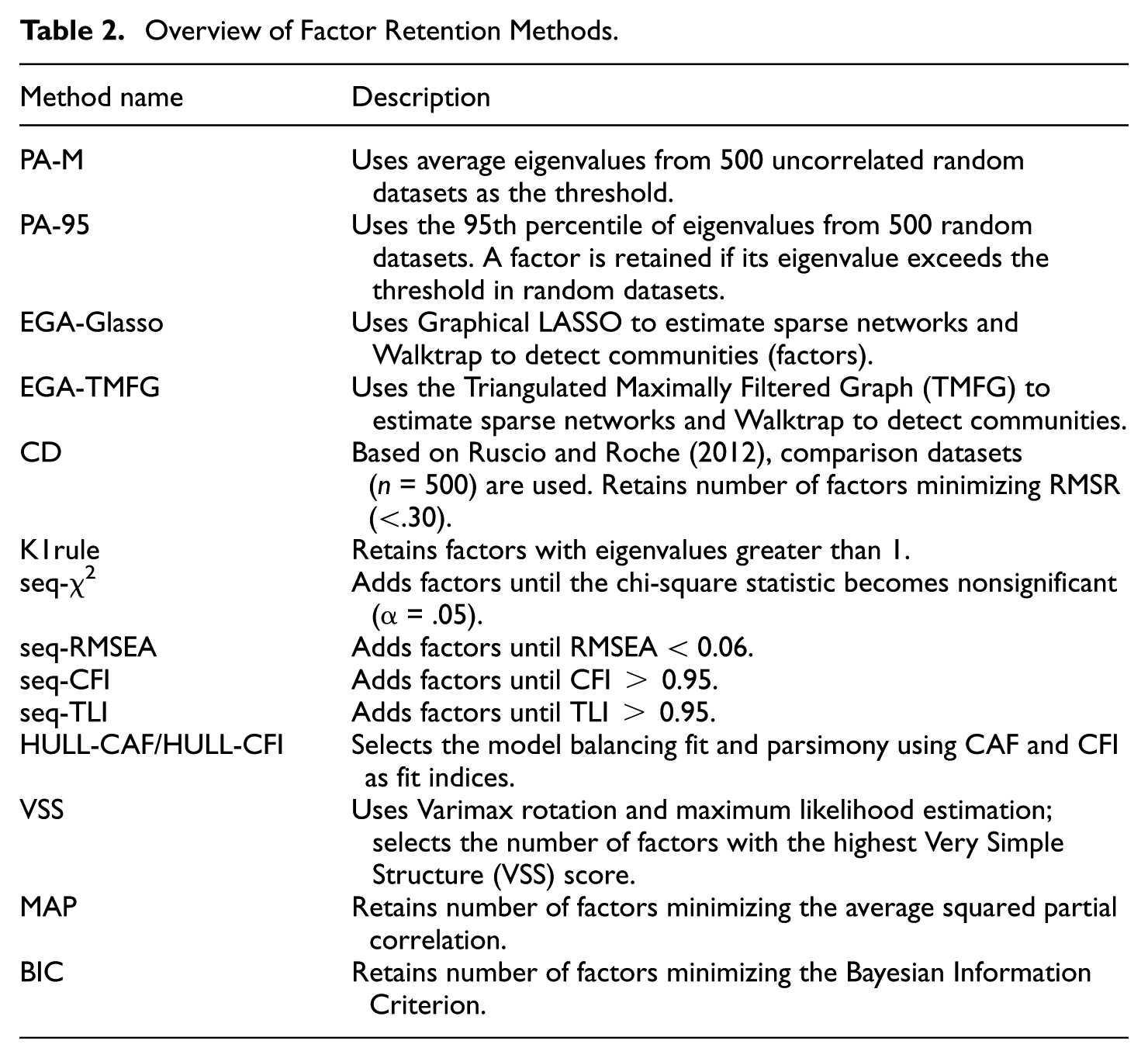
Currently, there exist several approaches to assist factor retention, which can generally be grouped into four families. The group includes simulation-based methods such as PA and comparison data (CD; Horn, 1965; Ruscio & Roche, 2012). The second group includes the traditional methods such as the scree plot, K1 rule, BIC (Bayesian information criterion), sequential chi-square tests (seq-χ²), sequential fit indices (seq-RMSEA, seq-CFI, seq-TLI), the Hull method, very simple structure (VSS) method, and minimum average partial (MAP) (Cattell, 1966; Kaiser, 1960; Lorenzo-Seva et al., 2011; Marsh et al., 2004; Preacher et al., 2013; Revelle & Rocklin, 1979; Velicer, 1976). Third, in recent decades, newer methods such as EGA have been developed, offering alternative approaches to dimensionality assessment (H. Golino et al., 2020). Fourth, machine learning techniques have also been introduced into factor retention research. For example, Goretzko and Bühner (2020) and Goretzko and Ruscio (2024) combined Machine learning algorithms and simulated data to determine the number of underlying factors. For a comprehensive overview of factor retention, Goretzko (2025) provides a detailed review of factor retention methods developed over the past century.

This study does not assume that all included methods represent equally strong contemporary contenders. Rather, the method set was chosen to balance methodological relevance with practical relevance. Some procedures, such as PA-based methods and EGA, are frequently discussed as strong performers in recent methodological work (e.g., Auerswald & Moshagen, 2019; H. Golino et al., 2020), whereas others, such as K1 were retained because they remain historically important and are still commonly used in applied EFA practice (Goretzko et al., 2021). From this perspective, including older or more heavily criticized methods is still informative, because it allows the study to distinguish between procedures that continue to function as useful benchmarks and those whose weaknesses become especially evident under comparatively large-factor conditions.

PA-M, originally proposed by Horn (1965), is currently one of the most widely used factor-retention methods in exploratory factor analysis (Goretzko et al., 2021). Because of its generally strong performance in prior simulation studies (e.g., Auerswald & Moshagen, 2019; Lim & Jahng, 2019), PA-M is often treated as a benchmark against which newer methods are evaluated (Goretzko, 2025). Its key advantage is that it accounts for sampling fluctuation by comparing observed eigenvalues with those obtained from randomly generated datasets with uncorrelated variables. In Horn’s original formulation, a factor is retained when the observed eigenvalue exceeds the mean of the corresponding random eigenvalue distribution. However, this mean-based criterion has been criticized for potentially yielding overfactoring (Zwick & Velicer, 1986). To address this concern, Glorfeld (1995) proposed a more conservative variant, PA-95, which retains a factor only when the observed eigenvalue exceeds the 95th percentile of the random eigenvalue distribution; Glorfeld further noted that this criterion parallels a hypothesis-testing logic with a nominal Type I error rate of .05. Although Green et al. (2012) raised important concerns about traditional parallel analysis and proposed revised parallel analysis, the broader literature does not support dismissing traditional PA-based procedures a priori. Xia (2021), for example, noted that no factor-retention method consistently outperforms all others across every condition and summarized prior evidence showing that Horn’s traditional parallel analysis and its revised versions have generally produced among the most accurate conclusions. Xia (2021) further reported that when only a trivial model misfit is present, traditional PA may be less sensitive than revised PA and may even achieve higher accuracy across most simulation conditions. Similarly, Goretzko and Bühner (2020) described parallel analysis as having become a kind of “gold standard” in the factor-retention literature, while also noting that newer methods tend to outperform it only under specific conditions. Taken together, the current literature supports including both PA-M and PA-95 as important reference methods and does not justify assuming that they will necessarily perform poorly before they are evaluated under the specific large-factor conditions considered in this study.

Ruscio and Roche (2012) proposed CD that follows the same statistical logic as PA, which is based on simulated comparison datasets. While PA compares eigenvalues from the real dataset to those from randomly generated datasets, CD generates datasets from the marginal distribution using a bootstrap method, which is believed (Ruscio & Kaczetow, 2008) to better approximate the structure of the real data in nonnormal distributions. CD then uses the root mean square residual (RMSR) to create RMSR distributions for both the real and simulated datasets and applies the Mann–Whitney U test to compare solutions with J (the current number of factors) and J + 1 (one additional factor). If the test is significant, indicating the current factor structure is inadequate, the method continues adding factors until the result is no longer significant. In previous research (Auerswald & Moshagen, 2019), CD performed well when there was sufficient information (e.g., more factors and larger sample sizes). Although CD generally did not perform as well as PA in previous studies (Lim & Jahng, 2019), it is still considered an acceptable alternative among simulation-based retention methods.

Recently, network psychometrics has emerged as an alternative approach to dimensionality assessment. EGA, introduced by Golino and Epskamp in 2017, is a method for factor extraction based on network analysis. It uses the Gaussian graphical model (GGM) to estimate the network structure through conditional dependencies. GGM can be estimated using one of the two methods: Graphical Least Absolute Shrinkage and Selection Operator (Glasso) or the Triangulated Maximally Filtered Graph (TMFG). In the Glasso approach, referred to as EGA-Glasso, a regularization parameter is used to minimize the extended Bayesian information criterion (EBIC), thereby controlling the sparsity of the network. The TMFG approach, referred to as EGA-TMFG, constructs the network by iteratively adding variables with the strongest correlations, ensuring a sparse and interpretable structure. Specifically, TMFG begins with one variable and connects it only to those with a high association. Once the network structure is estimated, the Walktrap algorithm is applied to detect latent factors by identifying clusters of strongly connected variables. EGA-Glasso outperforms PA-M when the correlation between factors is .5 and .7 in a four-factor model (H. F. Golino & Epskamp, 2017).

Older procedures such as the Kaiser–Guttman rule were included for a different reason. We did not retain them because we expected them to outperform more modern approaches. Rather, they were included because they remain highly visible in applied EFA practice and therefore remain relevant to the audience this paper is intended to serve. Recent review evidence suggests that the continued use of older factor-retention methods is not limited to a single field. In psychological research, Goretzko et al. (2021) found that the Kaiser–Guttman rule remained the most commonly used retention criterion, followed by the scree test and parallel analysis. In cyberpsychology and human–computer interaction, Howard (2016) similarly concluded that researchers often continued to rely on outdated retention methods, revealing a persistent gap between methodological recommendations and actual practice. In management research, Howard (2023), based on a review of 1,790 articles and 3,396 EFAs, likewise found that many widely recommended EFA guidelines were still infrequently applied and that more recent methodological developments had not yet been broadly adopted. Taken together, these reviews indicate that older methods remain relevant in applied research, providing a clear rationale for retaining traditional procedures such as the Kaiser–Guttman rule in the present comparison.

Apart from the parallel-analysis and network-based families, several other methods included in this study are based on maximum likelihood estimation (MLE) (Lawley, 1940). The first is the seq-χ ² , which evaluates whether the empirical covariance matrix from the original dataset fits the model-predicted covariance matrix. This is done using MLE, followed by a likelihood ratio test to assess model fit. The seq-χ² proceeds in a stepwise manner: it begins with a one-factor model, and if the test is significant, indicating poor fit, one additional factor is added. This hypothesis testing process continues until the model with the added factor provides an acceptable fit, and we conclude with the number of factors in the last model.

In addition to the seq-χ², sequential uses of fit indices such as the Comparative Fit Index (CFI; Bentler, 1990), Tucker–Lewis Index (TLI; Bentler & Bonett, 1980; Tucker & Lewis, 1973), and root mean square error of approximation (RMSEA; Steiger, 1990) have also been employed. These indices are often recommended in conjunction with the sequential chi-square test (Yang & Xia, 2015) as a way to mitigate the chi-square test’s sensitivity to slight misspecification under large sample sizes (e.g., Hu & Bentler, 1998). Although these three indices are widely used in factor analysis, they face challenges when applied to factor retention. One central limitation lies in the ambiguity of cutoff criteria: while Hu and Bentler (1999) suggested the cutoff values that have been widely adopted in practice, these cutoff values are not generalizable because they are influenced by incidental parameters such as factor correlations and factor loadings (Savalei, 2012). Because of this limitation, some researchers have continued to propose alternative approaches to utilize the fit indices, such as other dynamic criteria (McNeish & Wolf, 2023). Other methods—including the MAP (Velicer, 1976), HULL method (Lorenzo-Seva et al., 2011), VSS (Revelle & Rocklin, 1979), and BIC (Preacher et al., 2013)—have also been proposed. However, according to Goretzko (2025), their usage in applied research remains relatively limited. Readers interested in these methods are encouraged to consult the original sources for further details, but we still include these methods in our simulation because their performance in large factor models remains unexplored.

Several features of this method make the comparison substantively useful. First, some included procedures, such as PA-M, PA-95, EGA-Glasso, and EGA-TMFG, are commonly treated as major reference methods in the factor-retention literature. Second, several other procedures, including the K1 rule, VSS, Hull-CAF, Hull-CFI, MAP, BIC, chi-square tests, and fit-index-based approaches, remain historically influential or are still encountered in applied research, even when methodological reviews have questioned their general performance. Evaluating these methods together is therefore useful not because all of them are expected to perform equally well, but because they continue to shape applied practice and methodological comparison. Moreover, prior criticism alone does not establish how these methods behave under the comparatively large-factor conditions examined here. From this perspective, the contribution of the study is not limited to identifying a single best-performing rule but also to clarify how a broad set of historically important and practically relevant methods behaves across large multidimensional conditions.

To address this gap, we systematically evaluated the performance of 15 factor retention methods in large factor models, which include PA-M, PA-95, EGA-Glasso, EGA-TMFG, CD, seq-CFI, seq-TLI, seq-RMSEA, seq-χ², K1 rule, VSS, Hull method-CAF, Hull method-CFI, MAP, and BIC. Specifically, this study addresses the following research questions:

In this study, “combining methods” refers to using two approaches from the same methodological family—for example, PA-M and PA-95—to make a joint decision about the number of factors to retain, with the goal of improving accuracy under challenging conditions. From an applied perspective, the study further examines which methods are most suitable for large-factor models and which should be avoided under specific conditions (e.g., small sample sizes, high correlations, or low loadings).

Answering these research questions is critical because most existing methodological studies have focused on small or moderate factor structures, whereas large factor models are increasingly common in psychological, educational, and social science research. Without clear evidence on how existing factor retention methods perform under such conditions, researchers may arrive at poorly supported conclusions about the dimensional structure, leading to weaker construct representation and less informative follow-up modeling. By systematically comparing 15 methods across a wide range of large factor model conditions, this study contributes to the methodological literature on exploratory factor analysis and provides concrete evidence.

Method

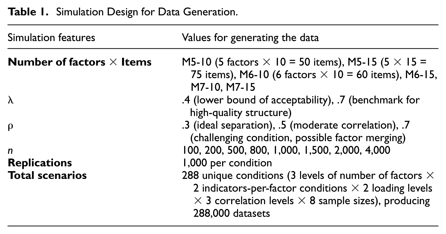
Data were generated following the specifications outlined in Table 1, and 15 factor retention methods were subsequently applied as described in Table 2. All simulations and analyses were conducted in R (Version 4.5.0; R Core Team, 2025).

OPEN IN VIEWER

Table 1.

Simulation Design for Data Generation.

Simulation features	Values for generating the data
Number of factors × Items	M5-10 (5 factors × 10 = 50 items), M5-15 (5 × 15 = 75 items), M6-10 (6 factors × 10 = 60 items), M6-15, M7-10, M7-15
λ	.4 (lower bound of acceptability), .7 (benchmark for high-quality structure)
ρ	.3 (ideal separation), .5 (moderate correlation), .7 (challenging condition, possible factor merging)
n	100, 200, 500, 800, 1,000, 1,500, 2,000, 4,000
Replications	1,000 per condition
Total scenarios	288 unique conditions (3 levels of number of factors × 2 indicators-per-factor conditions × 2 loading levels × 3 correlation levels × 8 sample sizes), producing 288,000 datasets

OPEN IN VIEWER

Table 2.

Overview of Factor Retention Methods.

Method name	Description
PA-M	Uses average eigenvalues from 500 uncorrelated random datasets as the threshold.
PA-95	Uses the 95th percentile of eigenvalues from 500 random datasets. A factor is retained if its eigenvalue exceeds the threshold in random datasets.
EGA-Glasso	Uses Graphical LASSO to estimate sparse networks and Walktrap to detect communities (factors).
EGA-TMFG	Uses the Triangulated Maximally Filtered Graph (TMFG) to estimate sparse networks and Walktrap to detect communities.
CD	Based on Ruscio and Roche (2012), comparison datasets (n = 500) are used. Retains number of factors minimizing RMSR (<.30).
K1rule	Retains factors with eigenvalues greater than 1.
seq-χ2	Adds factors until the chi-square statistic becomes nonsignificant (α = .05).
seq-RMSEA	Adds factors until RMSEA < 0.06.
seq-CFI	Adds factors until CFI > 0.95.
seq-TLI	Adds factors until TLI > 0.95.
HULL-CAF/HULL-CFI	Selects the model balancing fit and parsimony using CAF and CFI as fit indices.
VSS	Uses Varimax rotation and maximum likelihood estimation; selects the number of factors with the highest Very Simple Structure (VSS) score.
MAP	Retains number of factors minimizing the average squared partial correlation.
BIC	Retains number of factors minimizing the Bayesian Information Criterion.

Simulation Design

Consistent with our definition of large factor models in the Introduction, the simulation design varied two components of structural complexity: the number of latent factors and the number of indicators per factor. Specifically, we examined models with five, six, or seven factors and with 10 or 15 indicators per factor. These conditions were selected to represent comparatively large multidimensional EFA structures that remain plausible in applied research.

We constructed six population models varying in the number of factors and indicators per factor: M5-10 (5 Factors × 10 Indicators = 50 indicators), M5-15 (5 × 15 = 75), M6-10, M6-15, M7-10, and M7-15. Table 1 provides an overview of the simulation conditions.

Regarding factor loadings, we followed conventions found in applied research. Most psychological assessment reports standardized acceptable loadings (λ) in the range of .4 to .7 (Goretzko et al., 2021). To reflect this, we selected .4 to represent the lower bound of acceptability and .7 as a benchmark for high-quality factor structures. For inter-factor correlations (ρ), we selected values of .3, .5, and .7, which are commonly observed in empirical settings. A correlation of .3 is generally regarded as an ideal condition in which factors are clearly distinguishable. .7 represents a more challenging condition. The condition with λ = .7 and ρ = .3, therefore, serves as the baseline condition for comparison because this condition is expected to result in the most accurate factor retention. We then manipulated either the λ (from .7 to .4 while holding ρ constant at .3) or the ρ (from .3 to .5 or .7 while holding λ constant at .7) to investigate the λ and ρ influence of each parameter independently.

For the sample size, we included a wide range to capture conditions encountered in both small- and large-scale studies:100, 200, 500, 800, 1,000, 1,500, 2,000, and 4,000. Although sample sizes of 100 and 200 may be considered relatively small, such sample sizes are not uncommon in educational and psychological research.

All data were generated under the assumption of multivariate normality. The full simulation design resulted in 288 unique conditions, defined by the crossed combinations of number of factors (5, 6, or 7), indicators per factor (10 or 15), n (100, 200, 500, 800, 1,000, 1,500, 2,000, 4,000), ρ (.3, .5, .7), and λ (.4, .7). Each condition was replicated 1,000 times, producing a total of 288,000 datasets.

We applied 15 factor retention methods to each of the 288,000 simulated datasets. These methods were categorized into four families: PA, EGA, sequential procedures, and classical retention rules. Table 2 presents an overview of factor retention methods. In this study, “correct” refers to recovery of the known population factor structure in the simulation setting; it should not be interpreted as implying that a uniquely correct number of factors is directly observable in real data.

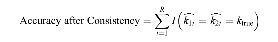
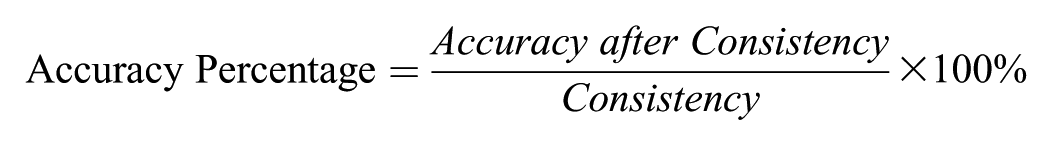
To improve factor retention accuracy under challenging conditions, we evaluated combination rules that integrate results from two methods within the same methodological family. Specifically, we examined the following pairwise combinations: PA-based (PA-M and PA-95) and EGA-based (EGA-Glasso and EGA-TMFG). We restricted the combinations to methods within the same family (e.g., PA-based or EGA-based), as cross-family combinations (e.g., PA with K1) generally showed lower consistency. Each combination was evaluated using three performance metrics—consistency, accuracy after consistency, and accuracy percentage (formula below) as proposed by Auerswald and Moshagen (2019). The combination rule was applied only when both methods produced the same factor solution; if their estimates differed, the replication was coded as inconsistent. These combination procedures were primarily examined under lower loading conditions (λ = .4), since when λ = .7, both PA and EGA methods performed well individually and did not require additional improvement through combination.

1. Consistency: defined as the number of replications (out of 1,000) in which both methods identified the same number of factors:

Consistency = ∑ i = 1 R I ( k 1 i ^ = k 2 i ^ )

2. Accuracy after consistency: the number of replications in which both methods agreed on the same number of factors, and that number matched the true factor number:

Accuracy after Consistency = ∑ i = 1 R I ( k 1 i ^ = k 2 i ^ = k true )

3. Accuracy percentage: the proportion of correct agreements among all consistent replications:

Accuracy Percentage = A c c u r a c y a f t e r C o n s i s t e n c y C o n s i s t e n c y × 100 %

Results

We summarize the main performance patterns in the text using three overview figures and reserve detailed condition-by-condition results for the online supplementary materials. Figure 1 shows each method’s overall profile across all simulation conditions in terms of correct recovery, overextraction, and underextraction. Here, “Correct” refers to recovery of the true number of factors, “Over” to retaining more factors than the true number, and “Under” to retaining fewer. Figures 2 and 3 show how correct recovery varies across the key design factors for the top five methods and the remaining methods, respectively. This presentation emphasizes the major trends while preserving full condition-level results in the appendix.

OPEN IN VIEWER

Figure 1.

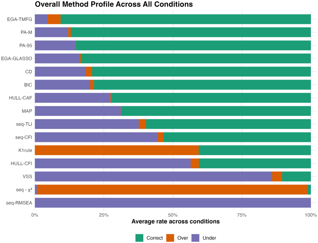
Global performance comparison of factor retention methods: Correct recovery, overextraction, and underextraction rates.

OPEN IN VIEWER

Figure 2.

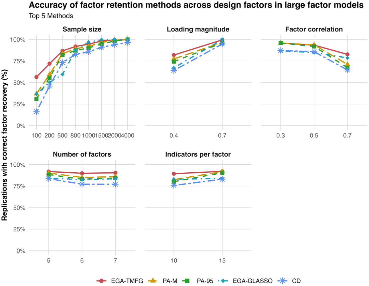
Effects of sample size, factor loadings, correlations, number of factors, and indicators per factor on correct recovery for top-5 performing methods.

OPEN IN VIEWER

Figure 3.

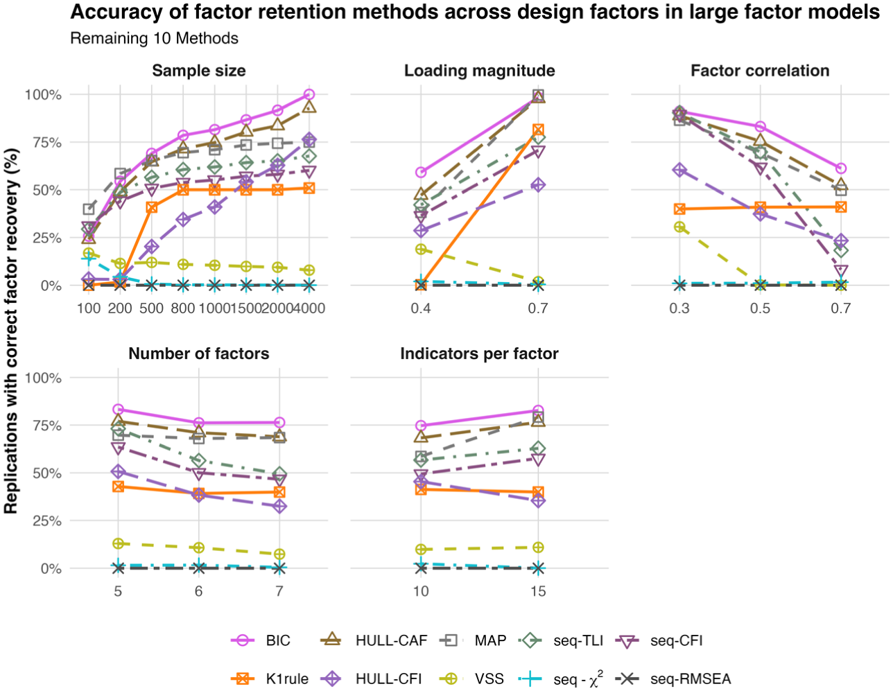
Effects of sample size, factor loadings, correlations, number of factors, and indicators per factor on correct recovery for the remaining 10 performing methods.

Figure 1 reveals a clear performance hierarchy. EGA-TMFG performed best overall, with about 90.7% correct recovery and balanced low rates of overextraction and underextraction (both about 4.5%). PA-M and PA-95 followed closely, with correct recovery rates of about 86.9% and 85.1%, respectively; for both methods, errors were driven almost entirely by underextraction, with negligible overextraction. EGA-Glasso and CD also remained competitive, with correct recovery rates of about 83.3% and 79.2%, although both showed somewhat greater underextraction.

Performance was less favorable for the remaining methods. BIC, Hull-CAF, and MAP formed a middle group, with correct recovery ranging from about 68.6% to 78.6%, again largely reflecting underextraction. Seq-TLI and seq-CFI performed more weakly, whereas K1 and Hull-CFI showed similar overall accuracy (about 40%) but opposite error tendencies: K1 mainly overextracted, whereas Hull-CFI mainly underextracted. The weakest methods were VSS, seq-χ², and seq-RMSEA. VSS recovered the correct number of factors in only about 10.3% of conditions, seq-χ² almost uniformly overextracted (98.0%), and seq-RMSEA almost uniformly underextracted (100%). Overall, the methods differed not only in accuracy but also in their characteristic error patterns.

Figure 2 shows that correct recovery for the five highest-performing methods is influenced most strongly by sample size, loading magnitude, and factor correlation, whereas the number of factors and indicators per factor has comparatively smaller effects. It presents correct recovery across key design factors for EGA-TMFG, PA-M, PA-95, EGA-Glasso, and CD, ordered by mean correct recovery across all simulated conditions. The panels summarize performance as a function of sample size, loading magnitude, factor correlation, number of factors, and indicators per factor. The y-axis represents the percentage of simulation replications in which a method recovered the correct number of factors, averaged over the remaining design factors.

Among these design factors, sample size showed the clearest and most systematic effect. EGA-TMFG was the least sensitive to smaller samples, increasing from about 57% at N = 100 to over 90% by N = 800 . PA-M and PA-95 followed similar but somewhat slower trajectories, rising from about 35% and 31% at N = 100 and reaching 90% at approximately N = 1 , 000 . EGA-Glasso improved from about 37% to 60% between N = 100 and N = 500 , but did not exceed 90% until around N = 1 , 000 . CD was the most sensitive to sample size, increasing from about 17% at N = 100 and reaching 90% only near N = 1 , 500 .

Loading magnitude showed a similarly strong effect. Increasing loadings from .40 to .70 raised correct recovery from about 82% to 99% for EGA-TMFG, from about 75% to 97% for PA-M, and from about 75% to 96% for PA-95. Larger gains were observed for EGA-Glasso (about 68%–99%) and CD (about 64%–95%), indicating greater sensitivity under weaker measurement conditions.

In contrast, higher factor correlations reduced performance. EGA-TMFG declined modestly (about 95%–83%), whereas PA-M and PA-95 showed larger decreases (about 95%–70% and 67%). EGA-Glasso declined from about 87% to 79%, and CD showed the largest drop (about 87%–65%).

By comparison, the number of factors and indicators per factor had smaller effects. EGA-TMFG remained stable across factor conditions (about 90%–92%), PA-M and PA-95 varied modestly (mid-80%–low-90%), and EGA-Glasso remained near 83% to 86%, whereas CD showed somewhat lower recovery. Increasing indicators per factor produced only moderate improvements across methods. Overall, EGA-TMFG, PA-M, and PA-95 showed the greatest robustness across conditions, whereas EGA-Glasso and especially CD were more sensitive under more difficult scenarios.

Figure 3 shows that lower-ranked methods were substantially less accurate and more sensitive to design conditions than the top-performing procedures. Among these methods, BIC, Hull-CAF, MAP, seq-TLI, and seq-CFI formed a relatively stronger subgroup, although their performance still varied considerably across conditions.

Sample size had a pronounced effect. BIC increased from about 30% correct recovery at N = 100 to 100% at N = 4000, exceeding 90% only at approximately N = 2,000. Hull-CAF rose from about 28% to about 92% across the same range, reaching 90% only at the largest sample size. MAP improved more modestly, from about 40% to about 75%, whereas seq-TLI and seq-CFI increased from about 16% to 67% and from about 28% to 60%, respectively. Overall, these methods required substantially larger samples to achieve acceptable performance and remained less stable than the top five methods.

Loading magnitude also had a strong influence. Increasing loadings from .40 to .70 raised correct recovery from about 58% to 100% for BIC, from about 47% to 98% for Hull-CAF, and from about 42% to 99% for MAP. Improvements were smaller for seq-TLI (about 40%–78%) and seq-CFI (about 36%–70%), again indicating greater sensitivity under weaker measurement conditions.

In contrast, higher factor correlations reduced performance for nearly all methods. BIC declined from about 91% at r = .30 to about 61% at r = .70, Hull-CAF from about 90% to 52%, and MAP from about 88% to 50%. The decline was more severe for seq-TLI (about 89%–20%) and especially seq-CFI (about 90%–about 9%), indicating substantial instability when factors were strongly correlated.

The number of factors and indicators per factor had smaller but still noticeable effects. Across five to seven factors, BIC, Hull-CAF, and MAP declined only slightly, whereas seq-TLI and seq-CFI showed clearer decreases. Increasing the number of indicators per factor from 10 to 15 generally improved performance for the stronger methods in this group, although gains were moderate.

The remaining methods were distinctly weaker. The K1 rule showed only moderate accuracy, increasing from about 2% at N = 100 to about 50% by N = 800 and remaining near that level thereafter, with little sensitivity to factor correlation. Hull-CFI performed somewhat better than K1 under some conditions but remained clearly below the more competitive procedures. VSS, seq-χ², and seq-RMSEA performed worst overall, with near-zero correct recovery across most conditions.

Overall, these results indicate that lower-ranked methods were not only less accurate on average, but also considerably more vulnerable to difficult design conditions, particularly small sample sizes, low loadings, and high factor correlations.

Figure 4 summarizes the within-family combination-rule results across all low-loading conditions (lambda = .4), aggregated across the six model structures and the three factor-correlation levels. The figure should be read as a retention plot: for each sample size, the y-axis represents the percentage of all replications retained at each stage of the combination rule. Thus, the first point corresponds to all replications (100%), the second point (“Same solution”) indicates the proportion of replications in which the two methods within the same family selected the same number of factors, and the third point (“Same solution and correct”) indicates the proportion of replications in which they agreed and that shared solution matched the true number of factors. For the PA-based family, the dominant pattern was relatively high within-family agreement across sample sizes. The PA-based combination retained a substantial proportion of replications even under small-N conditions, with about 44% of replications remaining at N = 100, 61% at N = 200, 79% at N = 500, and 85% at N = 800; agreement exceeded 90% by N = 1,500. However, agreement did not always imply correctness. The percentage of replications that were both consistent and correct was only 4.6% at N = 100, 26.0% at N = 200, 63.5% at N = 500, and 74.4% at N = 800, and it exceeded 90% by N = 2,000. Thus, the PA-based combination mainly contributed by providing a broadly applicable consistency rule, although its retained solutions were not uniformly correct at smaller sample sizes. The EGA-based family showed a different pattern. At very small sample sizes, EGA-Glasso and EGA-TMFG rarely agreed, with essentially no retained replications at N = 100 or N = 200. Even at N = 500, only about 18.4% of replications were retained. However, once the two EGA methods agreed, the retained solutions were close to correct. Specifically, the percentage of replications that were both consistent and correct was about 18.4% at N = 500 and 70.6% at N = 800, and it exceeded 90% by N = 1,500. Moreover, from N = 500 onward, the percentages for “Same solution” and “Same solution and correct” were nearly identical, indicating that once the EGA methods converged on the same solution, that solution was almost correct. In this sense, the EGA-based combination functioned less as a broad consistency filter and more as a highly selective rule with very high correctness among retained solutions.

OPEN IN VIEWER

Figure 4.

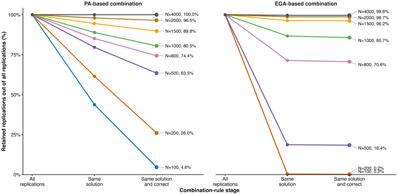
Consistency–selectivity trade-off in PA- and EGA-based combination rules under low-loading conditions.

Taken together, these figures suggest a clear hierarchy in method performance. EGA-TMFG, PA-M, PA-95, EGA-Glasso, and CD formed the strongest group overall, with relatively high recovery and greater robustness across the major design factors. The remaining methods performed less favorably and were more vulnerable to difficult conditions, often showing distinct tendencies toward overextraction or underextraction. Across the full set of methods, sample size, loading magnitude, and factor correlation were the primary drivers of performance differences, whereas the number of factors and the number of indicators per factor played comparatively smaller roles.

Discussion

This study compared 15 factor-retention methods in comparatively large factor models defined by both the number of factors and the number of indicators per factor. Overall, the results revealed a clear performance hierarchy. EGA-TMFG, PA-M, PA-95, EGA-Glasso, and CD formed the strongest group overall, whereas the remaining methods were more vulnerable to difficult conditions and more likely to show systematic overextraction or underextraction. Across methods, sample size, loading magnitude, and factor correlation emerged as the primary determinants of performance, whereas the number of factors and the number of indicators per factor played comparatively smaller roles. This pattern is consistent with prior simulation research showing that no single retention method performs best under every condition and that performance depends strongly on design features such as loading size, correlation, and sample size (Auerswald & Moshagen, 2019; Xia, 2021).

From a practical standpoint, the most informative comparison was concentrated among EGA-TMFG, PA-M, PA-95, EGA-Glasso, and CD. Within this group, PA-M and PA-95 performed especially well under low-to-moderate factor correlations, which is consistent with earlier findings from smaller-factor simulations (Auerswald & Moshagen, 2019; Lim & Jahng, 2019). In this study, PA-M generally remained slightly stronger than PA-95, suggesting that the traditional mean-based criterion still performs competitively in large-factor conditions, despite long-standing concerns that it may overextract. At the same time, the results also showed that PA-based methods became less competitive when factor correlations were high, particularly when loadings were low. This pattern is broadly consistent with prior work indicating that strong factor correlations make later dimensions harder to recover because the leading eigenvalues dominate the variance structure (Braeken & Van Assen, 2017). One interesting result in this study was that, under these more difficult high-correlation and low-loading conditions, increasing the number of indicators per factor improved the performance of PA-based methods, suggesting that the additional measurement information may partially offset the tendency toward underextraction in large-factor settings.

The network-based methods also showed a differentiated pattern that was partly consistent with previous findings and partly more specific to the present design. EGA-TMFG performed especially well under high-correlation conditions and was generally more stable than EGA-Glasso when information was limited, such as in smaller samples or under low loadings. This is consistent with H. Golino et al. (2020), who also found that EGA-TMFG can remain comparatively robust under more difficult conditions. By contrast, EGA-Glasso performed well when sample size was sufficient, but was clearly less reliable in large-factor models with smaller samples and low loadings. One particularly noteworthy finding was the nonconvergence of EGA-Glasso under these more difficult conditions, which is also compatible with earlier work showing lower convergence rates for EGA-Glasso when sample size and loading magnitude are small (H. Golino et al., 2020). A plausible explanation is that stronger regularization under limited-information conditions can overshrink the network, making it harder for the Walktrap algorithm to recover the latent structure. This interpretation is also consistent with Christensen et al. (2024), who suggested that the default tuning settings in EGA-Glasso may be overly aggressive. Thus, one substantive contribution of this study is to show that the relative strengths of EGA-TMFG and EGA-Glasso depend not only on factor correlation, but also on whether the available sample size is sufficient for stable network estimation in comparatively large-factor conditions. CD was also among the better-performing methods, although it was generally less competitive than PA-M, PA-95, and the stronger EGA procedures. Its overall pattern was most similar to the PA family, which is sensible given that both approaches are simulation-based. In this study, CD typically required more favorable conditions, especially larger sample sizes, to achieve acceptable recovery. This is consistent with earlier work showing that CD can perform reasonably well, but usually not as strongly as the best PA variants (Lim & Jahng, 2019). At the same time, one interesting result was that CD sometimes compared more favorably with PA under high-correlation conditions with strong loadings and limited sample size. Although this did not overturn the broader hierarchy, it suggests that CD may remain a viable alternative when researchers want a simulation-based method but do not wish to rely exclusively on the PA framework.

The lower-ranked methods were informative less because they competed with the top group and more because they showed distinct and often systematic error tendencies. This point is important because this study was designed not only to identify the strongest performers, but also to clarify how benchmark, traditional, and still-used methods behave in comparatively large-factor models. Several methods—including BIC, Hull-CAF, MAP, seq-TLI, and seq-CFI—showed acceptable performance only under relatively favorable conditions, such as high loadings and larger sample sizes. By contrast, seq-χ², seq-RMSEA, and VSS performed poorly across most of the design space. These findings are broadly compatible with previous concerns that fit-index-based or sequential fit-based rules may not be well suited for factor-retention decisions, especially when conventional cutoffs are imported from CFA without considering how strongly they depend on loading size, factor correlation, and other incidental parameters (McNeish & Wolf, 2023; Xia, 2021). In particular, seq-RMSEA showed severe underextraction, likely because the sequential procedure often terminated too early once conventional RMSEA thresholds were satisfied. Conversely, seq-χ² showed a strong tendency toward overextraction, which is consistent with its sensitivity to trivial misfit as sample size grows (Hu & Bentler, 1998). K1 also remained vulnerable to overextraction under low-loading conditions, although it performed better under easier conditions with high loadings and larger samples. Thus, the contribution of including these methods is not that they represent equally strong contemporary competitors, but that they remain visible in practice and display recognizable failure patterns that applied researchers should understand.

The combination-rule analysis provided an additional perspective under the most difficult low-loading conditions. The PA-based combination retained agreement across a larger proportion of replications, indicating greater within-family stability, whereas the EGA-based combination retained fewer replications but yielded a higher proportion of correct solutions. This pattern suggests that within-family agreement can serve different purposes depending on the method family: for PA-based methods, agreement appears to function as a relatively stable and inclusive filter, whereas for EGA-based methods, agreement appears to identify a smaller but more trustworthy subset of retained solutions. In this study, these combination rules were most relevant when loadings were low; when loadings were high, most leading methods already performed well individually, so combination offered little additional benefit.

More broadly, the present findings help clarify why a broader method set remains useful even when the main applied competition is concentrated among a smaller group of leading methods. Reviewer concerns that some included procedures are outdated or weaker are reasonable, but the present results show that their inclusion is still informative. Applied researchers continue to encounter older methods such as K1 and fit-based procedures, and the current study helps distinguish between methods that remain competitive, methods that can work only under favorable conditions, and methods that are especially prone to systematic over- or underextraction. In that sense, the contribution of the study is not limited to identifying a single best-performing method. Rather, it lies in showing how a broad set of benchmark, network-based, simulation-based, and still-used traditional procedures behaves in comparatively large multidimensional conditions, while also narrowing practical attention to the relatively small set of strongest competitors. This focus also aligns with the revised presentation of the results, which emphasizes overview patterns in the main text and leaves condition-level detail to the supplement. Importantly, accurate statistical recovery does not by itself guarantee substantive usefulness. In applied research, factor-retention decisions also depend on interpretability and theoretical meaningfulness.

Limitations

Several limitations of the current study should be acknowledged. First, the simulation study focused exclusively on normally distributed data. In practice, however, applied research often involves categorical data. Second, the simulations did not incorporate missing data, which is prevalent and can have a substantial impact in real-world datasets. Addressing missingness is crucial for evaluating the robustness and practical utility of factor retention methods. Third, the study did not examine more complex factor structures, such as multilevel models or those involving cross-loadings, which may influence method performance in different ways. Fourth, We acknowledge that this specification is more homogeneous than most applied datasets, in which factor loadings and correlations typically vary across indicators. Finally, future research should consider the inclusion of trivial model misfit during the data-generating process, as highlighted by Xia (2021), to better approximate conditions encountered in applied settings.

More recently, machine learning-based factor retention methods have been developed (Goretzko & Bühner, 2020). These methods involve training machine learning algorithms—often using random forest classifiers—on a wide range of data conditions (e.g., varying eigenvalues, RMSEA, sample sizes) to predict the optimal number of factors. While promising, these methods come with practical limitations. First, they require significant computational time and resources for model training. Second, they demand very large datasets to ensure stable and reliable predictions. Given these limitations, such methods are currently less feasible for use in applied psychological research and were therefore excluded from the present simulation study.