Differential test functioning (DTF) evaluates whether a test exhibits group differences beyond those attributable to latent trait differences. Its magnitude is often most interpretable on the raw-score scale. However, most existing DTF effect size measures rely on item response theory (IRT) modeling. Building on the renewed practical value of sum scores, this study proposes a simple observed-score-based approach to estimate the DTF magnitude directly in raw-score points. The proposed Index S stratifies examinees by an anchor-based sum score composed of items not flagged for differential item functioning (DIF), summarizes the within-stratum mean differences in total test scores, and aggregates these conditional differences using weights based on the observed distribution of the matching variable. To stabilize the estimation when score strata are sparse, adjacent strata are merged to satisfy a minimum per-group sample size requirement, and Index S_std provides a standardized version. We evaluated the indices using two-parameter logistic (2PL) simulation studies by varying the sample size, test length, DIF type, DIF proportion, DIF direction, and focal group latent trait distribution. The utility was assessed in terms of estimation accuracy, including Bias and root mean square error (RMSE), and correlation with established IRT-based DTF indices. An empirical application to TIMSS 2023 Grade 8 mathematics (Japan vs. the United States) illustrates how the proposed indices provide an accessible raw-score interpretation of the DTF magnitude for both psychometric and non-psychometric stakeholders.
When conducting differential item functioning (DIF) analyses in test development and related settings, it is important to examine not only DIF but also differential test functioning (DTF) (Drasgow et al., 2018; Stark et al., 2004). DIF refers to the simple observation that an item displays different statistical properties in different group settings after controlling for differences in group ability (Angoff, 1993). In this study, DTF similarly refers to the simple observation that the entire test displays different statistical properties across groups after controlling for latent trait differences using information from all items. A related concept is differential bundle functioning (DBF), which targets a subset of test items (e.g., a booklet) and estimates the magnitude of differential functioning within that subset. Although previous work has sometimes discussed DTF and DBF without making a strict distinction (Shealy & Stout, 1993), the present study distinguishes between the two and focuses specifically on DTF.
When the two respondent groups (a focal group and a reference group) are compared in the DIF analyses, two DIF patterns are possible. The first case is one in which DIF items favor, for example, the reference group, and the resulting DTF also favors the reference group; this is called unidirectional DIF (Raju et al., 1995). The second case occurs when items favoring the focal group and those favoring the reference group are balanced to a similar degree; this is called bidirectional DIF. In this situation, two items (one favoring the reference group to the same degree as another favoring the focal group) can cancel each other out, producing no net contribution to the total DTF (Raju et al., 1995). In addition, even when no single item is flagged as exhibiting DIF, the accumulation of small DIF effects may induce DTF at the test level (Stark et al., 2004). Because decisions are made based on the results of an entire test rather than on the results of individual items, DTF analysis plays a critical role in ensuring test fairness (Chalmers et al., 2016; Pae & Park, 2006; Stark et al., 2004; Temel, 2023).
The estimation of DTF magnitude has been discussed primarily in terms of item response theory (IRT)-based parametric methods (Meade, 2010). Following Meade (2010), we introduce the signed test difference in the sample (), Stark’s differential test functioning ratio (; Stark et al., 2004), and the expected test score standardized difference ().
First, for , denotes the expected score () for respondent on item , evaluated at that respondent’s estimated latent trait level using the estimated focal-group item parameter . Similarly, denotes the corresponding ES computed using the estimated reference-group item parameter . The item-level signed item difference in the sample () for item is defined as
and is the sum of across the items
is designed so that the advantages and disadvantages within an item between the reference and focal groups can offset each other. , formed by summing across items, also captures the cancelation of DIF effects. This feature is useful for evaluating the substantive impact of DTF in practical contexts such as when comparing group means at the entire test level.
Next, let the test characteristic curve (TCC) represent the expected total test score for the reference group at a particular value of the latent trait, and let represent the TCC value for the focal group, computed using the equated focal group item parameters. The in raw-score points can then be obtained by integration, as shown here
where is the ability density for the focal group, which is assumed to be normally distributed with a mean of and a variance of 1. Essentially, the represents the difference in how the underlying attribute relates to the expected observed scores of the two groups (Stark et al., 2004).
Finally, using the expected test score (), the is defined as
and can be interpreted analogously to Cohen’s (Cohen, 1988). and are unstandardized effect sizes on the raw-score scale, whereas is standardized and therefore useful when comparing DTF magnitudes across tests or scales with different numbers of items.
Recently, the intuitive interpretability and practical utility of sum scores have been re-evaluated. Sijtsma et al. (2024) showed that raw scores stochastically order latent trait values and position sum scores as robust ordinal approximations of continuous latent traits. Their simulations further showed that the correlation between sum scores and true , or , often exceeds the correlation between estimated and true , or especially with small sample sizes or misspecified item response functions (Sijtsma et al., 2024). In addition, from the perspective of intuitive test theory, sum scores are readily interpretable because performance is expressed directly in raw-score units (Braun & Mislevy, 2005; Sijtsma et al., 2024). Applied to the DTF estimation, one can state, for example, that in a 20-point test, the magnitude of the DTF is approximately three points. Such raw-score interpretation helps not only psychometricians but also non-psychometrician practitioners and test stakeholders grasp the DTF magnitude more easily (Baguley, 2009). Simultaneously, sum scoring corresponds to a constrained measurement model and is not assumption-free; therefore, its use should be justified relative to the intended inferential goal (McNeish & Wolf, 2020). Therefore, in the present context, we adopted a simple, observed-score-based approach to summarize test-level differential functioning on the raw-score scale, rather than pursuing latent trait estimation itself.
However, most DTF estimation methods proposed to date are IRT-based (Chalmers et al., 2016; Halpin, 2024; Meade, 2010). SIBTEST is a well-known standardization-based procedure that evaluates differential functioning by separating items into a studied or suspect subtest and a valid or matching subtest (Shealy & Stout, 1993). A distinctive feature of SIBTEST is its regression correction, which adjusts for residual group differences in target ability after matching on the valid subtest. Although SIBTEST can be configured to evaluate the collective differential functioning of multiple studied items at the subtest or test level, it was primarily developed as a hypothesis-testing framework and typically handles sparse score strata by excluding them from the computation. In contrast, the present study focused on an effect-size summary expressed directly as raw-score points for the entire test. SIBTEST’s primary emphasis on hypothesis testing was beyond the scope of this study.
Recent work on DTF has proposed methods that account for sampling variability and provide confidence intervals for DTF magnitude (Chalmers et al., 2016), as well as methods that avoid the explicit identification of anchor items in DIF/DTF analyses (Halpin, 2024). These are important contributions to uncertainty quantification and address the practical difficulties of anchor-item selection. In addition, while IRT-based frameworks such as differential functioning of items and tests (DFIT) provide well-established test-level indices (e.g., signed and unsigned TCC-based measures) (Raju, 1988; Raju et al., 1995), these methods require fitting an IRT model and computing the ES functions. The contribution of the present study is that it provides a purely observed-score, standardization-based effect-size summary of the DTF magnitude that can be computed without IRT modeling, while retaining raw-score interpretability and the cancelation property emphasized in the DTF literature.
Accordingly, this study proposes a simple approach for DTF analysis based on sum scores and the corresponding magnitude of the DTF indices (Index and Index ). Index first stratifies respondents by scores on non-DIF items (anchor items) and then aggregates within-stratum mean differences in total test scores to estimate the magnitude of DTF, while controlling for latent trait distribution differences between the focal and reference groups contained in the observed mean score difference. Index is a standardized version of Index . Methodologically, we evaluated (a) estimation accuracy based on and root mean square error (); (b) correlations with established IRT-based indices (); and additional sensitivity analyses. We also illustrate how Index can be interpreted using real large-scale assessment data from TIMSS 2023 Grade 8 Mathematics (Japan vs. the United States).
This study contributes to the literature by (a) providing an effect-size index that allows for intuitive interpretation of DTF magnitude on a raw-score scale and (b) establishing the potential for complementary use with existing IRT-based DTF indices. We did not directly compare methods that focused primarily on confidence intervals for DTF magnitude (Chalmers et al., 2016) or methods that do not require the explicit identification of anchor items (Halpin, 2024). Instead, we focus on IRT-based point-estimate DTF indices () and limit the scope to developing and validating the Index which can approximate these existing indices.
Index Procedure
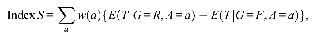
The Index proposed in this study aims to summarize the test-level score difference attributable to DIF (i.e., the DTF component) on a raw-score scale. As the observed mean score difference combines both the impact (differences in ability distributions) and DTF effects (Stark et al., 2004), we stratified respondents by anchor item scores and estimated the DTF component by aggregating within-stratum raw-score differences using weights proportional to group sizes.
Conceptually, Index is a standardization-based estimator that summarizes the conditional mean difference in total scores across groups after matching on an anchor-based score and then averages these conditional differences using the observed distribution of the matching variable. This perspective links the proposed index to the long-standing standardization approach in DIF research (Dorans & Kulick, 1986) and to SIBTEST’s model-based standardization framework, which separates the impacts of DIF and DIF/DTF components (Shealy & Stout, 1993).
More formally, let denote the anchor-score stratum, the observed total test score, and group membership. Index can be written as
where denotes the weight assigned to anchor-score stratum . In the present study, corresponds to the pooled observed distribution of the anchor score. Thus, Index is a direct standardization estimator that averages anchor-score-specific differences in total scores over the observed distribution of the matching variable.
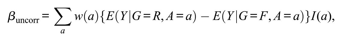
This formulation also clarifies the relationship between Index and SIBTEST-type estimators. In the usual SIBTEST procedure, regression correction is typically incorporated to adjust for residual group differences in target ability after matching (Shealy & Stout, 1993). To isolate the direct standardization component and clarify the algebraic relationship with Index , consider an uncorrected SIBTEST-type standardization estimator using the same matching variable and weights. The corresponding quantity can be written as
where denotes the studied item or studied subtest score and is an inclusion indicator for whether stratum is retained in the computation. Therefore, when for all strata, the same weights are used, and regression correction is not applied. Index is algebraically equivalent to the corresponding uncorrected direct-standardization estimator.
In general, however, Index is not identical to the usual SIBTEST β. The usual SIBTEST framework is defined for a studied item or studied subtest score, assumes a distinction between the studied and valid/matching subtests, incorporates regression correction in its standard formulation, may exclude sparse strata from the computation of β when the number of examinees in a stratum falls below a minimum per-group sample size, denoted , and provides a formal significance test in addition to an estimate of DIF/DTF magnitude (Bolt & Stout, 1996; Shealy & Stout, 1993). By contrast, Index , as proposed here, is an observed-total-score effect-size summary designed to quantify DTF magnitude directly in raw-score units, without an accompanying hypothesis-testing procedure.
Assuming two respondent groups of interest, Index is computed in the following three steps:
First, conduct DIF analysis and identify non-DIF items as anchor items.
Second, we computed the anchor item total score and stratified the respondents in one-point increments. For each stratum, the mean difference in total test scores between the groups was calculated and weighted by the proportion of respondents in that stratum.
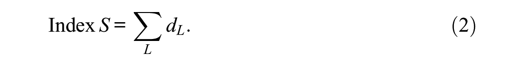
Third, the weighted values across all strata were summed to obtain the Index , an indicator of the DTF magnitude. If required, the standardized indicator Index can also be computed by dividing Index by the pooled standard deviation of the total test scores across the groups.
Because Index and Index summarize the test-level DTF impact, DIF effects can cancel out across items regardless of whether the DIF is unidirectional or bidirectional. Thus, they share the same cancelation properties as , and .
Step 1: Identification of Anchor Items
Before the DTF analysis, a DIF analysis was conducted to identify the anchor items. Existing DIF methods, such as the Mantel–Haenszel (MH) method (Mantel & Haenszel, 1959) and Raju’s method (Raju et al., 1995), can be used.
Step 2: Stratification by Anchor Items and Computation of Mean Sum-Score Differences
For each respondent, we computed the total anchor item score identified in Step 1 and stratified the respondents according to that score in one-point increments. Within each stratum, we computed the mean difference in total test scores between the two groups. To ensure a minimum per-group sample size, denoted , in each stratum, adjacent strata were merged whenever the count fell below . Specifically, we proceeded from lower to higher scores and, as a rule, merged an underpopulated stratum with the adjacent higher-score stratum (); only for the topmost stratum, where upward merging was not possible, we merged downward (). This merging was repeated until all the resulting strata met the criterion. Because the goal was to quantify the test-level DTF magnitude, we did not exclude sparse strata from the analysis (Shealy & Stout, 1993). This choice differs from the SIBTEST inclusion-rule approach, in which score categories that do not satisfy the minimum sample-size requirement may be omitted from the computation. We adopted merging rather than exclusion to retain the full observed-score range when summarizing DTF magnitude on the total-score scale.
Then, for each stratum formed by the anchor-item total score, compute
where denotes the stratum defined by the total anchor item score. Within each stratum, , , and represent the mean total test scores for the reference and focal groups, respectively, and denotes the proportion of respondents in that stratum among all respondents.
Step 3: Computation of DTF Magnitude Indices
Based on Step 2, compute DTF magnitude indices as follows:
As is clear from Equations 1 and 2, Index is a raw-score-based DTF index whose unit depends on the number of items in the test. In other words, it is an unstandardized index with benefits such as ease of interpretation (Baguley, 2009). However, their magnitudes cannot be compared directly across tests or scales with differing numbers of items.
Therefore, as a standardized index,
Index can also be proposed. This is a standardized DTF index, analogous to derived from IRT, and can be interpreted in a manner similar to Cohen’s (Cohen, 1988).
Simulation Studies
In this study, the utility of the proposed indices (Index and Index ) was evaluated from two perspectives: (a) estimation accuracy and (b) correlations with existing IRT-based DTF indices. These primary simulation studies assumed that the anchor items were correctly identified, thereby allowing the basic estimation performance of Index to be evaluated under controlled conditions. To address practical implementation issues, we also conducted an additional targeted sensitivity analysis examining the effects of anchor contamination and the choice of , the minimum per-group sample size required within each anchor-score stratum. A representative condition is reported in the main text, and the full set of conditions is provided in the Supplemental Material.
Perspective (a) evaluates and, while Perspective (b) provides convergent validity evidence relative to established indices. Simulations were performed using the mirt package (Chalmers, 2012), version 4.4.2 in R (R Core Team, 2025). IRT-based indices () were derived from a two-group two-parameter logistic (2PL) model estimated with multipleGroup() and computed using empirical_ES(). Their signs were adjusted as needed to ensure a consistent direction of interpretation with Index and Index . The EM algorithm was used for estimation; non-DIF (anchor) items were constrained to be invariant across groups, and the focal-group mean and variance were freely estimated. Population benchmark values were defined using large Monte Carlo samples (50,000 per group) and therefore did not depend on the finite-sample conditions. The default EM convergence criterion in mirt (tolerance (TOL) = .0001) was used because the convergence tolerance was not explicitly specified in the estimation call.
Design
This simulation study used dichotomous response data. Responses were generated using the 2PL IRT model.
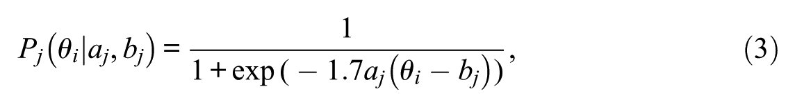
Under this model, the probability of a correct response on an item is defined as a logistic function of a respondent’s latent trait parameter theta , item discrimination parameter , and item difficulty parameter .
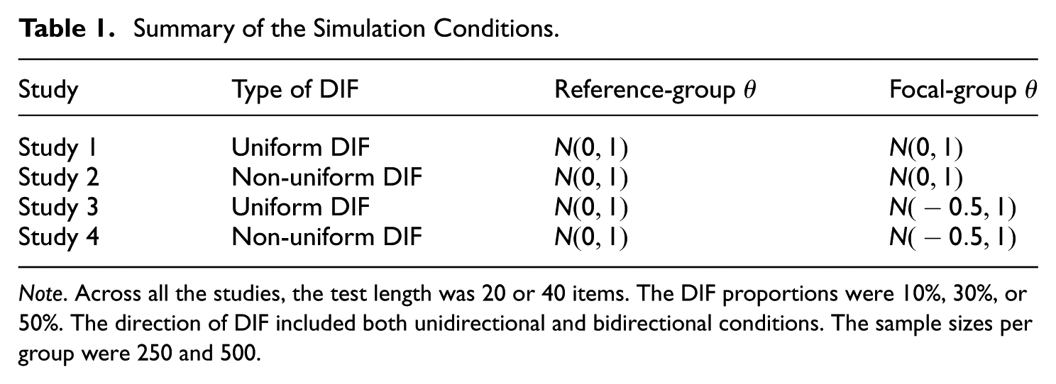
We simulated the responses for the two groups (reference and focal) with N = 250 or 500 respondents per group. We manipulated six factors: sample size (250 or 500 per group), test length (20 to 40 items), type of DIF (uniform or non-uniform), proportion of DIF items (10%, 30%, or 50%), direction of DIF (unidirectional or bidirectional), and latent trait distribution of the focal group (s; ). The latent trait distribution of the reference group was fixed at . The simulation design is presented in Table 1.
Summary of the Simulation Conditions.
Study
Type of DIF
Reference-group
Focal-group
Study 1
Uniform DIF
Study 2
Non-uniform DIF
Study 3
Uniform DIF
Study 4
Non-uniform DIF
Note. Across all the studies, the test length was 20 or 40 items. The DIF proportions were 10%, 30%, or 50%. The direction of DIF included both unidirectional and bidirectional conditions. The sample sizes per group were 250 and 500.
Specifically, the test length was set to 20 or 40 items, and the DIF proportions were 10%, 30%, or 50%. DIF items were placed in the latter part of the test. For example, when the test length was 20 and the DIF proportion was 30%, Items 15–20 (six items) were set as DIF items.
We assumed two types of DIF: uniform DIF and non-uniform DIF. For the item parameters, under uniform DIF, the parameters were set identically for both groups. When the test length was 20 items, the first 10 items were set to = 1.2, and the remaining 10 items were set to = 1.8. When the test length was 40 items, the first 10 items were set to = 1.2, and the remaining 20 items were set to = 1.8. The parameters were also identical across groups; we repeated the sequence ( = –1, –0.5, 0, 0.5, and 1) until the required number of items was reached. We then introduced DIF by shifting the difficulty of the DIF items by (+ 0.5).
Under non-uniform DIF, the baseline item-parameter settings were the same as those used for uniform DIF. For DIF items, however, we induced non-uniform DIF by varying the parameter across subgroups using the pairs ( = (1.2, 1.5), (1.5, 1.8), (1.8, 1.2)) repeated as many times as needed to cover the designated number of DIF items. For example, with a 20-item test and a DIF proportion of 30%, six items (Items 15–20) were designated as DIF items. In the non-uniform DIF condition, their parameters were assigned across subgroups as (= (1.2, 1.5), (1.5, 1.8), (1.8, 1.2), (1.2, 1.5), (1.5, 1.8), (1.8, 1.2)).
Regarding the direction of DIF, we specified two conditions: unidirectional DIF, in which all DIF items were shifted for Group 2 such that , and bidirectional DIF, in which DIF items were split evenly so that half were shifted for Group 1 (), and the other half were shifted for Group 2 ().
For the latent-trait distribution, we considered two conditions: (a) Both groups followed a standard normal distribution , and (b) only Group 2 had a shifted mean of .
Evaluation Criteria
The estimation accuracy evaluation focused on Index versus and , and on Index versus . Owing to space limitations, we report the results only for Index and in the main text; the results for and are provided in the Appendix and Supplemental Materials.
For each simulation condition (sample size, test length, proportion of DIF, type of DIF, direction of DIF, and the focal group’s latent trait distribution), let denote the estimate obtained in replication (), and let denote the true value under condition . and were computed as
The true value was numerically approximated using a large Monte Carlo sample (50,000 respondents per group) generated with the item-parameter settings for each condition. In computing the true values, responses were generated by assigning the same latent trait distribution to both groups so that the resulting values reflected only the DTF component, with the impact component (i.e., between-group ability differences) removed. Therefore, the true values did not depend on the sample-size condition . In this study, we set .
The true value of is defined as the expected difference in test scores under the 2PL model in Equation (3).
and were numerically approximated using the same distribution. Correspondingly, s and for were computed as follows:
Notably, even in conditions where the latent trait distributions of the two groups differed (Studies 3 and 4), the true values were defined under the same distribution. This choice was made so that the true value would represent the DTF component attributable to DIF itself, rather than a mixture of DTF and between-group differences in latent trait distributions. Thus, Studies 3 and 4 were designed to evaluate whether each index could accurately recover the DTF component even when impact was present in the estimation sample.
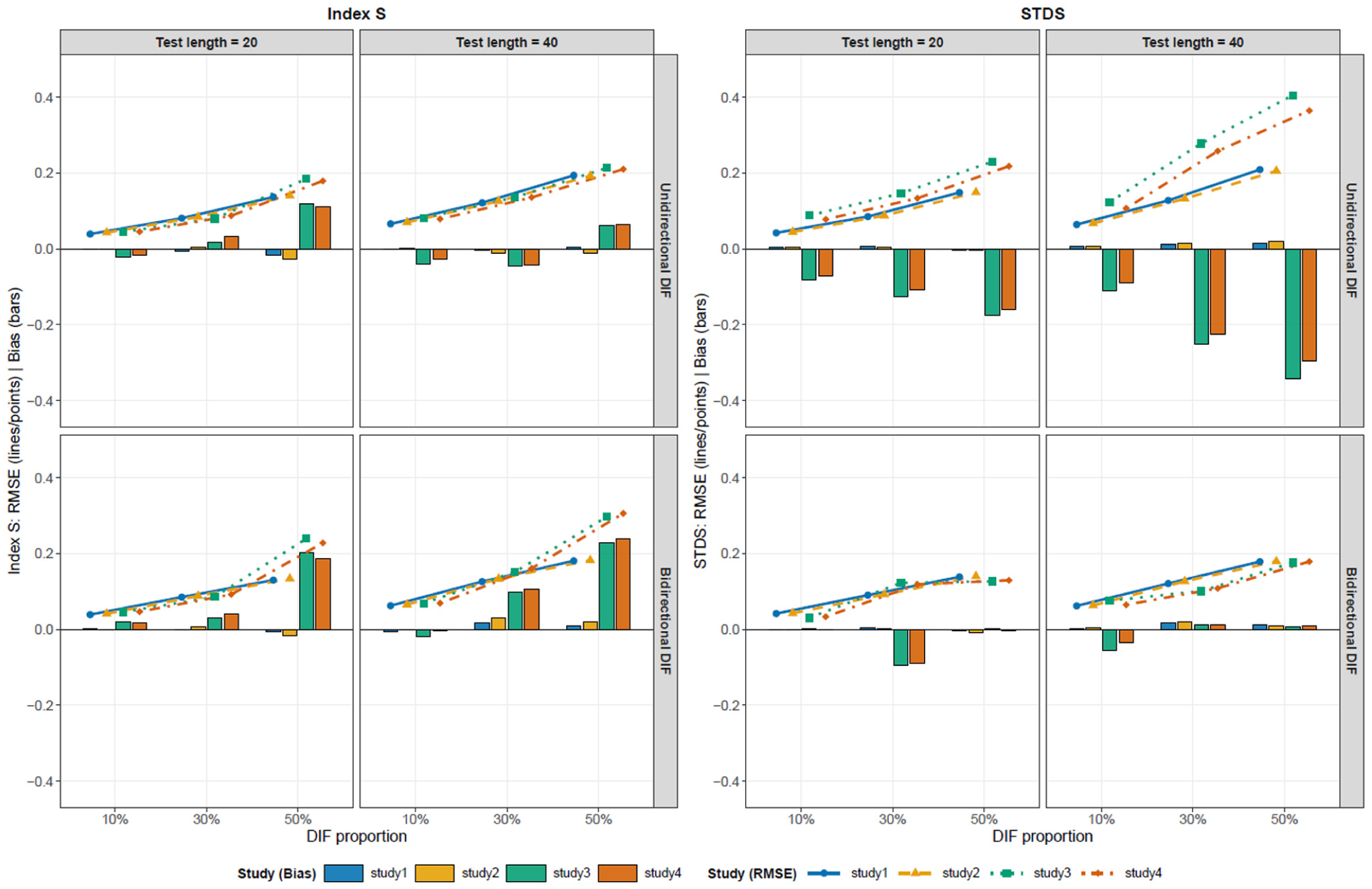
Results: (a) Estimation Accuracy
Figures 1–4 show the estimation accuracy of S and STDS in terms of (lines) and (bars) across the four sample-size conditions ( 250/250, 250/500, 500/250, and 500/500). Detailed numerical results for each condition, as well as the results for Index versus and Index versus , are provided in the Supplemental Materials. Although there are multiple ways to set (Chalmers & Zheng, 2023), we adopt , which is the most aggressive setting (Shealy & Stout, 1993).
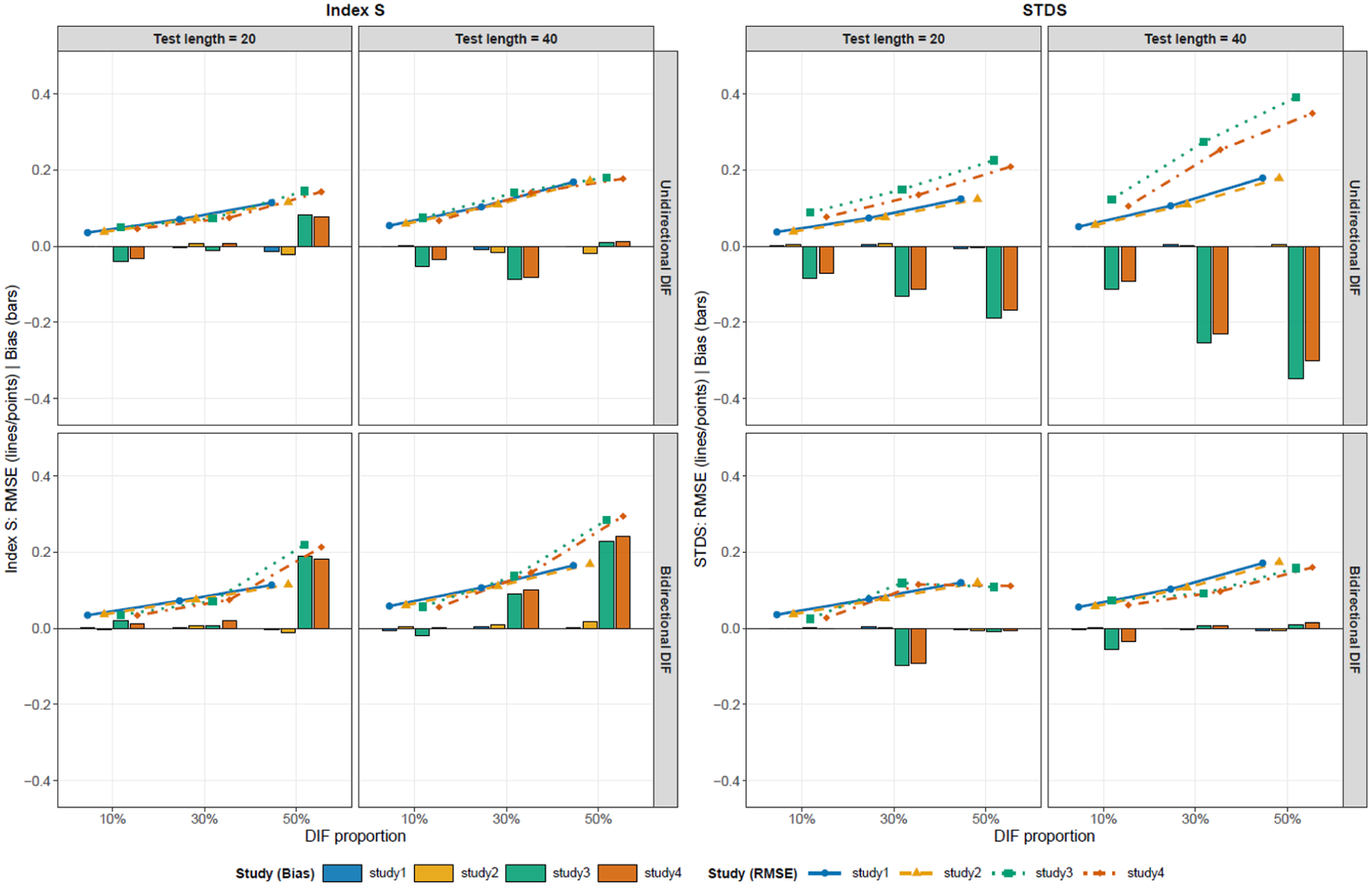
and of Index and (.
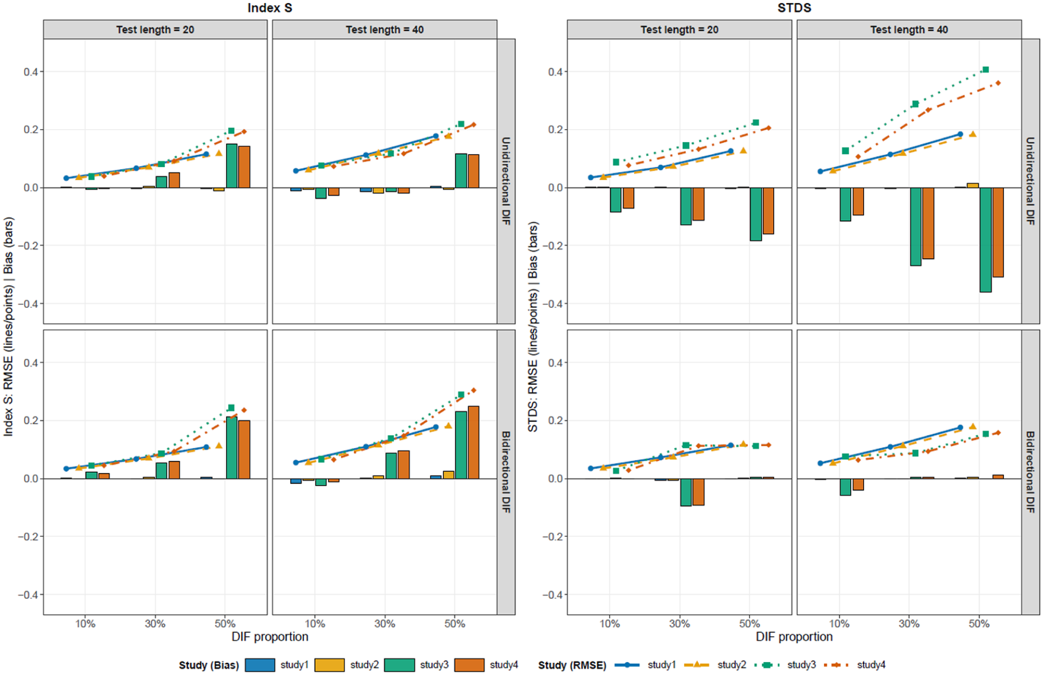
and of Index and (.
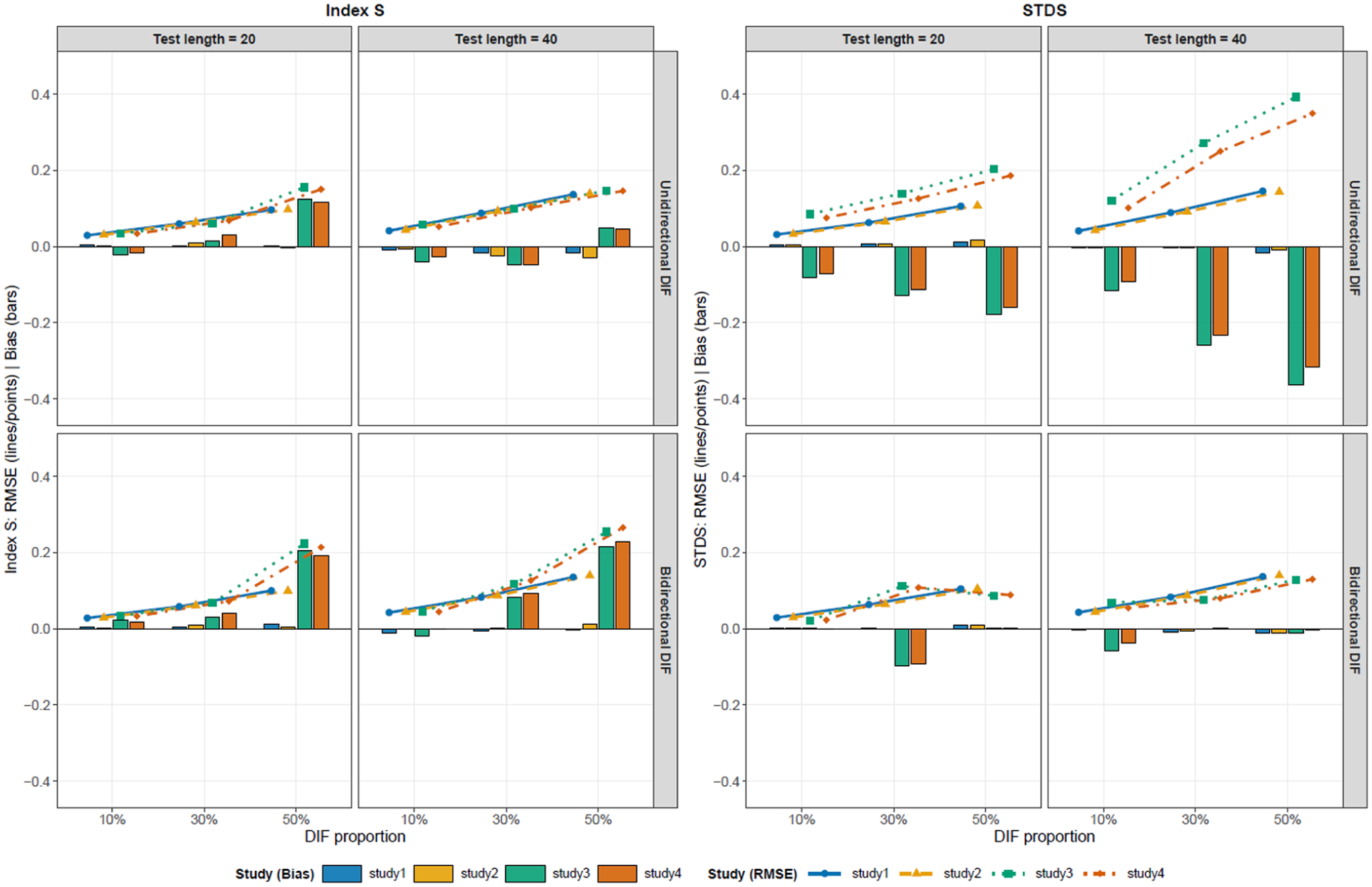
and of Index and (.
and of Index and (.
As shown in Figure 1, , increased for both indices as the proportion of DIF increased. For , the increase was relatively larger under latent mean-shift conditions (Studies 3 and 4) with unidirectional DIF, and this pattern was particularly pronounced when the test length was 40. With respect to, Index generally remained near zero, whereas a positive emerged under the latent mean-shift conditions with bidirectional DIF at the 50% DIF condition. In contrast, showed a consistently negative under latent mean-shift conditions with unidirectional DIF.
As shown in Figure 2, , again increased with the proportion of DIF, consistent with Figure 1. Index exhibited relatively stable behavior under this condition, whereas continued to show an inflated and persistent negative under latent mean-shift conditions with unidirectional DIF.
In Figure 3, and did not deteriorate substantially overall; however, its positive became relatively larger under the latent mean-shift conditions with bidirectional DIF. tended to yield a comparatively larger among the four sample size conditions, and its negative persisted under latent mean-shift conditions with unidirectional DIF.
In Figure 4, for , the estimation variability is generally reduced when both groups have larger sample sizes. The Index showed the most stable performance across the four conditions, with limited . Nevertheless, even under this condition, still exhibited an increased and a persistent negative under latent mean-shift conditions with unidirectional DIF.
Overall, both indices exhibited an increasing as the proportion of DIF increased. In addition, differences between indices were dependent on the conditions. For , an inflated and a consistently negative were observed under latent mean-shift conditions (Studies 3 and 4) with unidirectional DIF. In contrast, Index generally maintained a relatively small across many conditions, although a positive was observed in Studies 3 and 4 with bidirectional DIF when the DIF proportion was 50%. These results suggest that estimation accuracy varies not only with the proportion of DIF but also with the combination of latent mean-shift conditions and the direction of DIF. Finally, the impact of parameter differences was relatively small compared to the effects of latent mean shifts and the direction of the DIF.
These systematic bias patterns can be understood as arising from differences in how the indices separate the DTF component from impact. For , anchor items in the multiple-group IRT model place the two groups on a common latent trait scale, but they do not make the group latent trait distributions identical. Because is a sample-based index that averages expected-score differences over the empirical distribution of estimated values, its averaging distribution may still reflect impact. When the expected-score difference function varies across , this sample-based weighting can produce systematic bias; in the present unidirectional DIF conditions, it appeared as negative and increased .
Index , in contrast, conditions on anchor-score strata before aggregating group differences. This design compares groups within the same anchor-score levels and is therefore intended to reduce the impact component before summarizing DTF magnitude. However, the anchor score is only an observed-score proxy for the latent trait. When the DIF proportion is high, the anchor set becomes smaller, and anchor-score matching becomes coarser; under bidirectional DIF, the cancelation of DIF effects may also be incomplete within each anchor-score stratum. These mechanisms provide a conceptual explanation for why Index S showed bias under latent mean-shift conditions with bidirectional DIF; in the present simulations, this Bias was positive, particularly under the 50% DIF condition.
Results: (b) Correlations With Existing Indices
Next, we analyzed the correlations between Index , Index , and existing DTF indices. The number of simulation replicates per condition was 500.
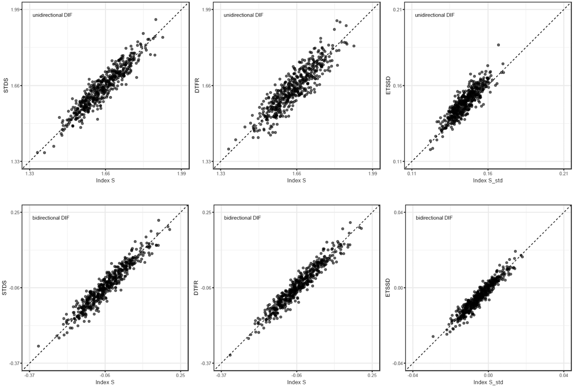
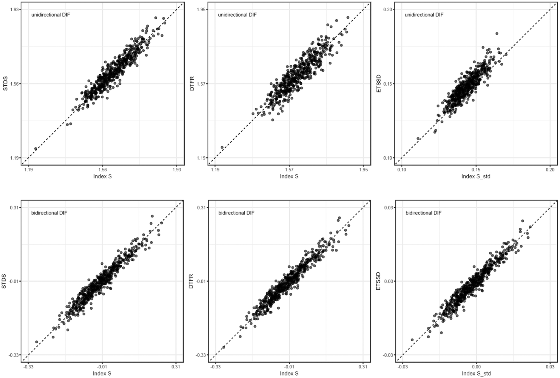
In Study 1, the correlations between Index and were high across all simulation conditions, ranging from a minimum of .854 to a maximum of .957. Similarly, the correlations between the Index and were high, ranging from .856 to .971. In addition, the correlations between the standardized Index and ranged from .785 to .957, indicating that the standardized index exhibited strong associations with the established indices. Figure 5 presents scatterplots for the condition in which both groups had sample sizes of , the test length was 40, the proportion of DIF was 30%, and the direction of DIF was either unidirectional or bidirectional. Scatter plots and a complete list of correlation coefficients for the remaining conditions are provided in the Supplemental Materials.
Scatterplots of Index and Index versus IRT-based DTF indices () for Study 1 ( per group; test length = 40; DIF proportion = 30%), shown separately for unidirectional and bidirectional DIF.
In Study 2, we examined the same set of conditions as in Study 1 but specified the type of DIF as non-uniform. The results again indicated strong correlations; across all simulation conditions, the correlations between Index and ranged from .877 to .965. Similarly, the correlation between the Index and ranged from .877 to .970. In addition, the correlations between and ranged from .797 to .964, indicating that the standardized index also showed high correlations with the established indices. Figure 6 presents scatterplots for the condition in which both groups had sample sizes of , the test length was 40, the proportion of DIF was 30%, and the direction of DIF was either unidirectional or bidirectional. Scatter plots and a complete list of correlation coefficients for the remaining conditions are provided in the Supplemental Materials.
Scatterplots of Index and Index versus IRT-based DTF indices () for Study 2 (N = 500 per group; test length = 40; DIF proportion = 30%), shown separately for unidirectional and bidirectional DIF.
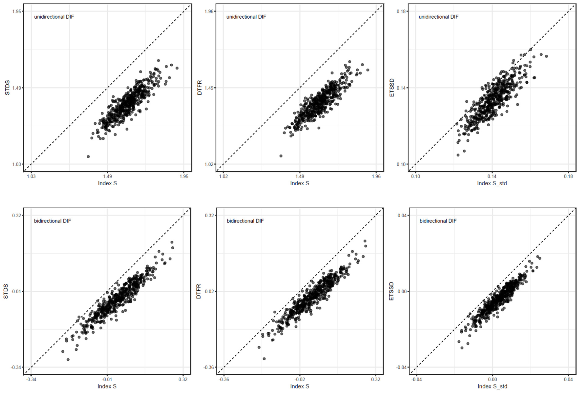
Study 3 corresponded to the subset of conditions in Study 1 in which the latent-trait distribution of Group 2 was set to . The simulation results indicated that across all conditions, the correlations between Index and ranged from .743 to .944, the correlations between Index and ranged from .760 to .946, and the correlations between the standardized index, Index , and ranged from .751 to .943. Although these correlations remained high, they were slightly lower than those observed in Study 1.
Figure 7 presents scatterplots for the same settings as in Figure 5, but under the latent-trait distribution . As shown, while the correlations remain high, the points appear to be systematically shifted such that Index tends to fall below the 45-degree line (i.e., in the lower-right region), which contrasts with the pattern observed in Figure 5.
Scatterplots of Index and Index Versus IRT-based DTF indices () for Study 3 ( per group; test length = 40; DIF proportion = 30%; Group 1: ; Group 2: ), shown separately for unidirectional and bidirectional DIF.
This combination of high correlations and systematic deviations from the 45-degree line is consistent with the estimation accuracy results based on and reported in Figures 1–4. Specifically, under the latent mean-shift condition, Index exhibited a positive in the bidirectional DIF condition, whereas exhibited a consistently negative in the unidirectional DIF condition, and an increased was also observed. Accordingly, the relationship between the indices in Study 3 can be interpreted as preserving rank-order agreement while showing reduced absolute agreement. That is, under latent mean-shift conditions, although the relative ordering of the respondents (or conditions) implied by the two indices was largely maintained, the index values themselves were more likely to diverge systematically in a directional manner.
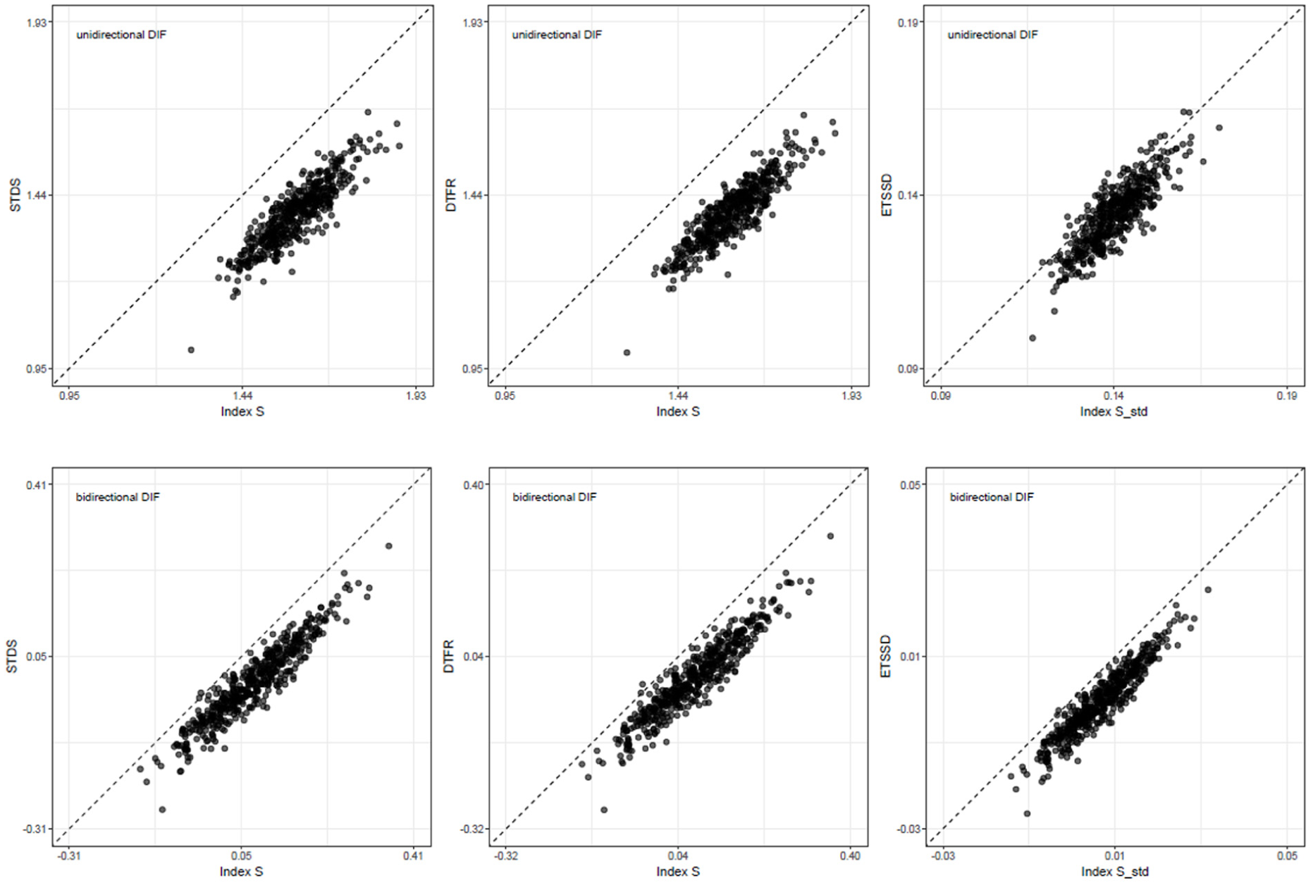
Finally, Study 4 corresponded to the subset of conditions in Study 2 in which the latent-trait distribution of Group 2 was set to . The simulation results indicated that across all conditions, the correlations between Index and ranged from .772 to .947; the correlations between Index and ranged from .782 to .953; and the correlations between the standardized index, Index , and ranged from .750 to .946. Although these correlations remained high overall, they were somewhat smaller than those observed in Study 2, mirroring the pattern found in the correlation results of Studies 1 and 3.
Figure 8 presents scatterplots for the same settings as in Figure 6 but under the latent-trait distribution . As shown, while the correlations remain high, Index again appears to be systematically shifted below the 45-degree line (i.e., in the lower-right region), which contrasts with the pattern in Figure 6. This tendency also parallels the relationship observed in Studies 1 and 3. These findings are consistent with the estimation accuracy results based on and .
Scatterplots of Index and Index versus IRT-based DTF indices () for Study 4 ( per group; test length = 40; DIF proportion = 30%; Group 1: ; Group 2: ), shown separately for unidirectional and bidirectional DIF.
Results: Additional Sensitivity Analysis
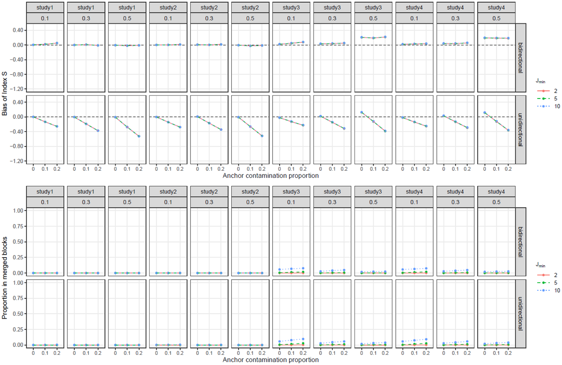
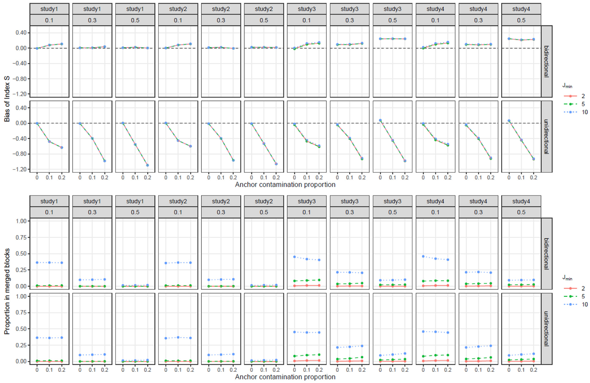
To address the practical issue that anchor items may not be perfectly identified in applied DIF analyses, we conducted an additional targeted sensitivity analysis. This analysis examined how Index was affected by anchor contamination and by the choice of The design crossed the four study conditions described earlier, test lengths of 20 and 40 items; group-size combinations of (250,250), (250,500), (500,250), and (500,500); DIF proportions of .10, .30, and .50; and unidirectional versus bidirectional DIF.
Anchor contamination was manipulated by replacing a proportion of the true anchor items with randomly selected DIF items while keeping the total number of anchor items constant. Three contamination proportions were examined: 0%, 10%, and 20%. We also varied across three values: 2, 5, and 10. For each condition, Index was evaluated in terms of , following the same definition used in the primary simulation studies. In addition, we recorded the proportion of examinees included in merged anchor-score blocks as a diagnostic of how much the sparse-stratum rule coarsened the matching variable. A representative figure is presented in the main text for the condition with 20 and 40 items and =500 per group, and the full set of conditions is provided in the Supplemental Materials.
Figures 9 and 10 summarize the additional sensitivity analysis for the representative sample-size condition with per group, separately for the 20-item and 40-item tests, based on 500 replications per condition. In each figure, the upper panel shows the of Index , and the lower panel shows the proportion of examinees included in merged anchor-score blocks. The same general pattern was observed across the full set of sample-size conditions reported in the Supplemental Materials.
Sensitivity of Index to anchor contamination and in the 20-item condition (. The column facets indicate the study number and DIF proportion (0.1, 0.3, and 0.5).
Sensitivity of Index to anchor contamination and in the 40-item condition ( The column facets indicate the study number and DIF proportion (0.1, 0.3, and 0.5).
Anchor contamination had a clear effect on Index , especially under unidirectional DIF. When no contaminated anchor items were included, was generally small, apart from the systematic patterns already observed in the primary simulation studies. As the contamination proportion increased from 0% to 10% and 20%, became increasingly negative under unidirectional DIF.
Under bidirectional DIF, the effect of anchor contamination was smaller and tended to appear as slightly positive rather than strongly negative . This pattern is consistent with the cancelation property of test-level DTF: When DIF effects operate in opposite directions, contaminated anchors may partly cancel at the total-score level, although such cancelation is not guaranteed within each anchor-score stratum. Thus, the impact of anchor contamination depended not only on the amount of contamination but also on the direction of DIF.
The sensitivity to was relatively limited with respect to . Across both test lengths, the curves for = 2, 5, and 10 were generally similar, suggesting that increasing did not systematically increase or decrease the of Index . In contrast, had a clearer effect on the stratification diagnostics. Larger values, especially = 10, increased the proportion of examinees included in merged anchor-score blocks, particularly in the 40-item tests. Thus, the main consequence of increasing was not a consistent change in , but a coarsening of the anchor-score matching due to more extensive stratum merging.
Empirical Application
To evaluate the practical utility of the proposed indices, we conducted an empirical analysis using real data. Specifically, we analyzed Booklet 1 from the TIMSS 2023 Grade 8 Mathematics Assessment for Japan () and the United States (). The booklet contains 43 items, including one polytomous item with three response categories (correct/partially correct/incorrect). For simplicity, partially correct responses were recorded as incorrect, and the items were treated as dichotomous. In addition, for item ID ME82511, all Japanese examinees had missing responses; therefore, this item was excluded from the analysis for both countries. The final analysis was based on 42 items.
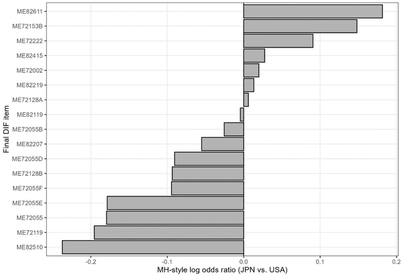
Before conducting the DTF analysis, we performed DIF analyses between the two countries, treating Japan as the reference group and the United States as the focal group. First, we applied the MH method (Mantel & Haenszel, 1959), Crossing SIBTEST (Li & Stout, 1996), and Raju’s method (Raju et al., 1995) using the difR package (Magis et al., 2010; version 6.1.0) in R (R Core Team, 2025). Items were classified as DIF items only when they were consistently flagged across all three methods; that is, when they were classified as category C (large effect) based on the ETS criterion in the MH method (Zwick, 2012) and were statistically significant in both Crossing SIBTEST and Raju’s method. All other items were used as anchors. Purification was performed using DIF procedures. As a result, 17 of the 42 items were detected as DIF items, leaving 25 anchor items. We also examined the direction of DIF among the 17 final DIF items using MH-style-matched odds ratios. This diagnostic suggested a mixed, rather than purely unidirectional, DIF pattern: Seven items favored Japan, and 10 items favored the United States. Although the DIF directions were mixed, the summed signed log odds ratios were larger in the U.S.-favoring direction, suggesting a net tendency for the DIF items to favor the United States. Figure 11 shows the MH-style log odds ratios for the final DIF items.
Direction of DIF among final DIF items based on MH-style matched odds ratios. Positive values indicate Japan-favoring DIF, and negative values indicate U.S.-favoring DIF.
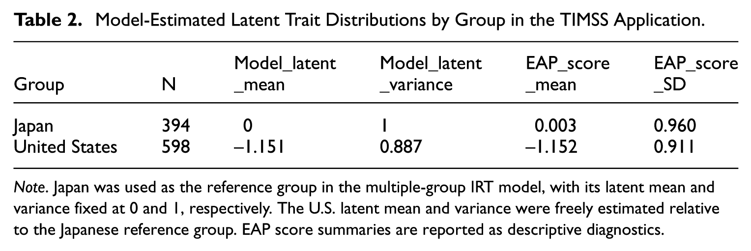
To diagnose the extent of impact in the empirical data, we also inspected the group latent trait distributions estimated from the multiple-group IRT model. As shown in Table 2, Japan served as the reference group, with its latent mean and variance fixed at 0 and 1, respectively. The U.S. latent mean was estimated to be –1.151, with an estimated variance of 0.887. The expected a posteriori (EAP) factor score summaries showed the same pattern. These results indicate a substantial latent trait distribution difference between the two groups in the analytic sample.
Model-Estimated Latent Trait Distributions by Group in the TIMSS Application.
Group
N
Model_latent_mean
Model_latent_variance
EAP_score_mean
EAP_score_SD
Japan
394
0
1
0.003
0.960
United States
598
–1.151
0.887
–1.152
0.911
Note. Japan was used as the reference group in the multiple-group IRT model, with its latent mean and variance fixed at 0 and 1, respectively. The U.S. latent mean and variance were freely estimated relative to the Japanese reference group. EAP score summaries are reported as descriptive diagnostics.
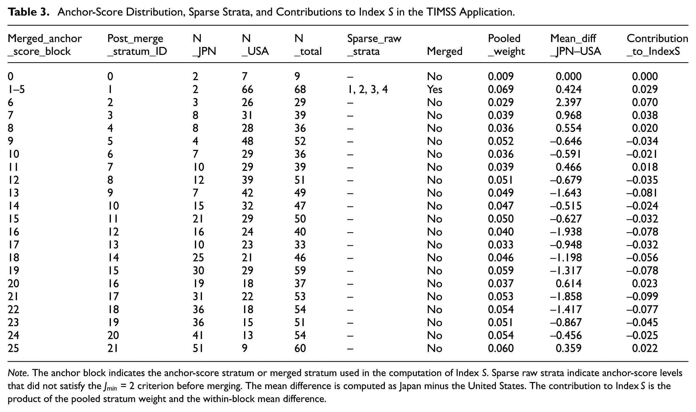
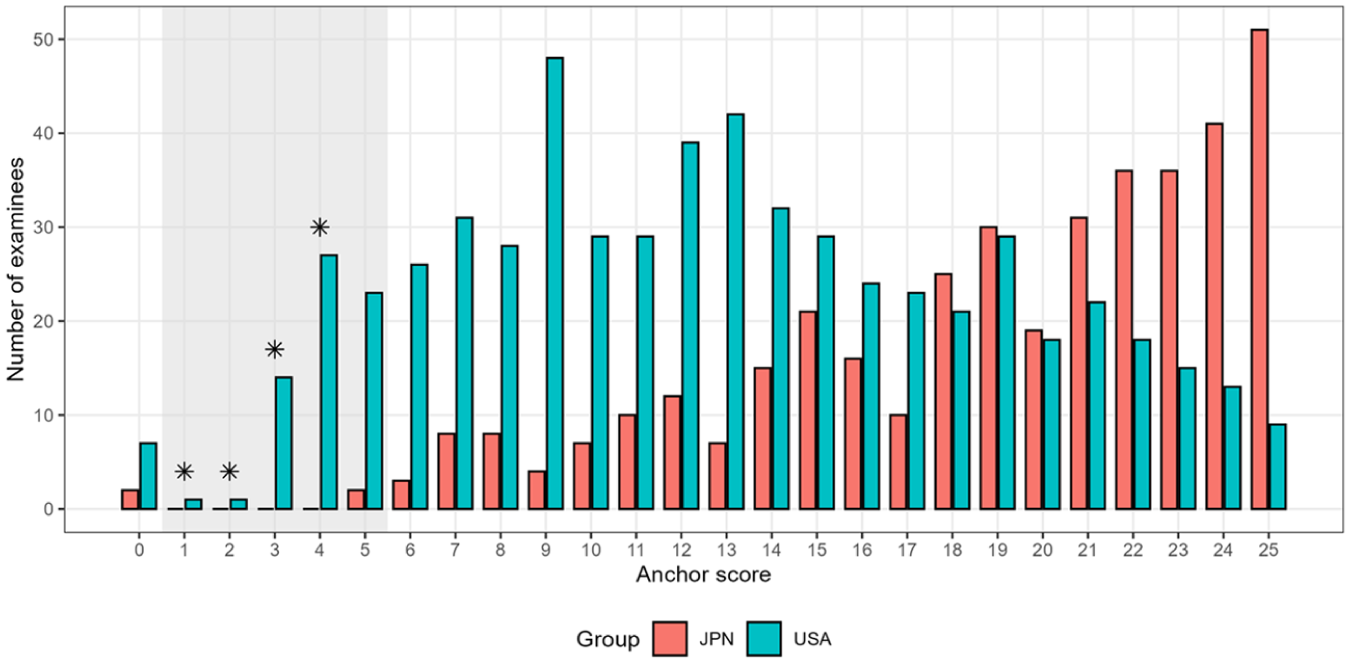
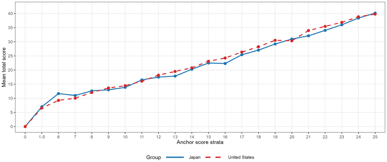
For the DTF analysis, we computed the proposed indices, Index and Index, using stratification based on the anchor item total score. To further evaluate the stability of the observed-score standardization, we examined the anchor-score distribution used for the computation of Index . The anchor-score distribution contained 26 raw strata, ranging from 0 to 25. Four raw strata, corresponding to anchor scores of 1–4, were sparse before merging because no Japanese examinees fell into these strata. These strata were therefore combined with the adjacent score level, resulting in one merged block covering anchor scores 1–5. After this merging step, 22 anchor-score blocks were used in the computation of Index . No other anchor-score blocks required merging. Table 3 summarizes the anchor-score stratification, Figure 12 displays the anchor-score distribution by group, and Figure 13 presents the mean total test scores for each stratum.
Anchor-Score Distribution, Sparse Strata, and Contributions to Index in the TIMSS Application.
Merged_anchor_score_block
Post_merge_stratum_ID
N_JPN
N_USA
N_total
Sparse_raw_strata
Merged
Pooled_weight
Mean_diff_JPN–USA
Contribution_to_IndexS
0
0
2
7
9
–
No
0.009
0.000
0.000
1–5
1
2
66
68
1, 2, 3, 4
Yes
0.069
0.424
0.029
6
2
3
26
29
–
No
0.029
2.397
0.070
7
3
8
31
39
–
No
0.039
0.968
0.038
8
4
8
28
36
–
No
0.036
0.554
0.020
9
5
4
48
52
–
No
0.052
–0.646
–0.034
10
6
7
29
36
–
No
0.036
–0.591
–0.021
11
7
10
29
39
–
No
0.039
0.466
0.018
12
8
12
39
51
–
No
0.051
–0.679
–0.035
13
9
7
42
49
–
No
0.049
–1.643
–0.081
14
10
15
32
47
–
No
0.047
–0.515
–0.024
15
11
21
29
50
–
No
0.050
–0.627
–0.032
16
12
16
24
40
–
No
0.040
–1.938
–0.078
17
13
10
23
33
–
No
0.033
–0.948
–0.032
18
14
25
21
46
–
No
0.046
–1.198
–0.056
19
15
30
29
59
–
No
0.059
–1.317
–0.078
20
16
19
18
37
–
No
0.037
0.614
0.023
21
17
31
22
53
–
No
0.053
–1.858
–0.099
22
18
36
18
54
–
No
0.054
–1.417
–0.077
23
19
36
15
51
–
No
0.051
–0.867
–0.045
24
20
41
13
54
–
No
0.054
–0.456
–0.025
25
21
51
9
60
–
No
0.060
0.359
0.022
Note. The anchor block indicates the anchor-score stratum or merged stratum used in the computation of Index . Sparse raw strata indicate anchor-score levels that did not satisfy the = 2 criterion before merging. The mean difference is computed as Japan minus the United States. The contribution to Index is the product of the pooled stratum weight and the within-block mean difference.
Anchor-score distribution and merged strata by group in the TIMSS application. Bars represent the number of examinees in each anchor-score stratum for Japan and the United States. The shaded region indicates the merged anchor-score block used in the computation of Index . Asterisks indicate raw anchor-score strata that did not satisfy the = 2 criterion before merging.
Mean test scores for Japan and the United States by anchor-item strata in the computation of Index S for TIMSS 2023 Grade 8 mathematics (Booklet 1).
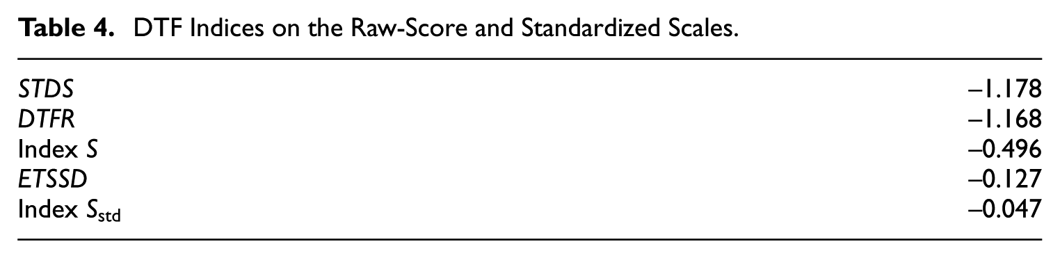
Next, we computed the IRT-based DTF effect-size indices () and a standardized index () using the mirt package (Chalmers, 2012) and compared them with Index and Index (Table 4). The signs of the IRT-based indices were oriented to match the sign convention of Index , so that all indices could be interpreted in the same direction. The results were , , and Index . Thus, on the raw-score scale (maximum score = 42), the magnitude of DTF was approximately 0.5 to 1.2 points, and all indices led to the same directional interpretation that the overall impact at the test level was limited. For the standardized indices, and Index , both of which fall within the small-effect range.
DTF Indices on the Raw-Score and Standardized Scales.
–1.178
–1.168
Index
–0.496
–0.127
Index
–0.047
The discrepancy between STDS and Index should be interpreted in light of the empirical conditions observed in the TIMSS data. The dataset involved both a high DIF proportion and substantial group differences in the matching variable and model-estimated latent trait distribution. Specifically, 17 of the 42 items were classified as DIF items, corresponding to a DIF proportion of 40.5%. In addition, the multiple-group IRT model estimated the U.S. latent mean to be approximately –1.15 relative to Japan, indicating substantial impact in the analytic sample. The MH-based direction diagnostic further suggested a mixed rather than purely unidirectional DIF pattern: Seven DIF items favored Japan, and 10 favored the United States. These empirical conditions are close to the high-DIF and latent mean-shift conditions examined in the simulation studies. Consistent with the simulation results, the accuracy and absolute magnitude of the indices may therefore have been more sensitive to DIF direction and to the distribution used for matching or averaging.
Index and STDS yielded the same directional interpretation, but Index was substantially closer to zero. Specifically, ∣Index ∣/∣∣ = .42. This suggests that, relative to , Index attenuated the absolute magnitude of the negative DTF estimate. One plausible explanation is that the high DIF proportion reduced the size of the anchor set and made anchor-score matching less precise, while the mixed DIF pattern allowed partial cancelation of DIF effects within anchor-score strata. This attenuation is consistent with the simulation findings showing that, under high-DIF and latent mean-shift conditions, Index may become biased when anchor-score matching becomes less precise and DIF effects cancel imperfectly within strata. Under such conditions, Index may have been shifted upward, thereby making the negative estimate less negative.
At the same time, the discrepancy should not be attributed solely to potential bias in Index . is also a sample-based index that averages expected-score differences over the empirical distribution of estimated values. Because the U.S. latent trait distribution was estimated to be substantially lower than the Japanese distribution, may also reflect the distribution over which the DTF function was averaged. Therefore, the discrepancy between and Index likely reflects a combination of the high DIF proportion, substantial impact, mixed DIF direction, and differences in the estimands and weighting schemes of the two indices. Because the true DTF value is unknown in the empirical data, the discrepancy should be interpreted as evidence that absolute DTF magnitudes can differ across indices under high-DIF and substantial-impact conditions, rather than as evidence that one estimate is definitively correct.
Discussion
This study proposed a simple approach for the DTF analysis method based on sum scores and the corresponding magnitude of DTF indices (Index and Index ) and examined their validity via simulation studies from three perspectives: (a) estimation accuracy (), (b) their relationships with existing IRT-based indices (), and additional sensitivity analyses of anchor contamination and . We conducted an empirical application using operational test data by applying both the proposed indices and IRT-based indices to evaluate their practical utility.
From the perspective of (a) estimation accuracy, and increased as the proportion of DIF increased, with error inflation becoming particularly pronounced under high-DIF conditions (30%–50%). A similar pattern was observed for (and for and ; see the Appendix and Supplemental Materials), although the form of the error depended on the condition. Specifically, (a) under unidirectional DIF combined with latent mean-shift conditions, showed marked increases in and a negative , whereas (b) under bidirectional DIF combined with latent mean-shift conditions, Index tended to exhibit an increasing positive . These results suggest that even with the same proportion of DIF, the pattern of estimation error differs across indices depending on the combination of DIF direction and the latent trait distributions of the groups being compared.
One possible contributor to this error pattern is that, as the proportion of DIF items increases, the purity of stratification based on anchor-item scores may deteriorate, making it more likely that the within-stratum mean differences are contaminated by residual DIF or DTF components. This mechanism is consistent with evidence from the SIBTEST literature that standardization-based approaches can deteriorate when the proportion of DIF items is large, partly because the matching variable becomes contaminated and the separation of impact and DIF/DTF components weakens (Gierl et al., 2004). In particular, an increase under the 50% DIF condition implies a heightened risk of overestimating the magnitude of the DTF when interpreting the point estimates of the index in practice. Therefore, caution is warranted when applying the proposed indices to high-DIF environments.
Regarding (b), the relationships between the proposed indices and existing DTF indices showed overall favorable associations, indicating rank-order agreement. However, absolute agreement tended to decline, especially under latent mean-shift conditions. Accordingly, in applied settings, it may be preferable to use indices and Index in conjunction with other DTF indices for a more comprehensive evaluation.
The additional sensitivity analysis also provides practical guidance for anchor selection and the choice of . Because anchor contamination directly affected the of Index , especially under unidirectional DIF, anchor selection should not be treated as a purely mechanical preprocessing step. When anchor items are not known a priori, researchers should use established DIF-detection procedures with purification and should report how the final anchor set was selected. Regarding , the sensitivity analysis showed that increasing from 2 to 5 or 10 did not systematically reduce ; the curves were generally similar across values. Because larger values increased stratum merging without consistently reducing Bias, = 2 appears to be a reasonable minimal default. Larger values should be used cautiously and, if considered, reported as part of a sensitivity analysis rather than being treated as default settings.
The empirical application further illustrated the practical interpretive value and limitations of Index . Although Index and the IRT-based indices yielded the same directional interpretation, their absolute magnitudes differed. As discussed in the empirical application, this discrepancy should be interpreted considering the high DIF proportion, substantial group differences in the anchor-score and latent trait distributions, mixed DIF direction, and differences in the estimands and weighting schemes of the indices. Thus, the empirical example supports the complementary use of Index with IRT-based DTF indices, especially in high-DIF or substantial-impact settings.
Index was developed to provide a simpler way to estimate the magnitude of DTF using raw scores without relying on IRT modeling. Its primary advantages are ease of estimation and intuitive interpretability. For example, as demonstrated in the empirical application, expressing the test-level DTF as “approximately 0.5 to 1.2 points on a 42-point test between Japan and the United States” provides an interpretation accessible to non-psychometric stakeholders such as test developers, educators, and policymakers (Baguley, 2009). In contexts where DTF is a concern, it is important to conduct DTF analyses alongside DIF analyses (Drasgow et al., 2018; Stark et al., 2004), and our results underscore that applied decisions are best supported by triangulation across multiple DTF indices.
From a computational perspective, Index is also less demanding than IRT-based DTF indices once the anchor set has been specified. Its computation requires only observed-score operations: computing anchor and total scores, tabulating respondents by anchor-score strata and group, calculating within-stratum total-score mean differences, and taking a weighted average of these differences. It does not require iterative latent-variable model fitting, estimation of item parameters, estimation of individual latent trait scores, or computation of ES functions. By contrast, IRT-based indices such as , , and require fitting an IRT or multiple-group IRT model and then computing ES or TCC differences. These steps can involve non-trivial computational cost, convergence checks, and model-fit considerations, especially in large simulation studies or more complex item-response models.
This computational advantage should be interpreted with one qualification. If anchor items are not prespecified, a DIF analysis is still required to identify the anchor set. Thus, the total computational burden depends partly on the DIF detection method used in Step 1. However, after the anchor set has been determined, Index itself can be computed with simple tabulation and weighted averaging, making it more accessible for applied settings in which full IRT modeling may be impractical.
This study has several limitations. First, this study focused on two-group comparisons. Extending the approach to multigroup settings is an important direction for future research. Although the logic of conditioning on anchor-score strata can, in principle, be extended to more than two groups, additional work is needed to define appropriate group comparisons, weighting schemes, and summary measures of test-level differential functioning in multigroup contexts. Second, our simulations were based on IRT, and we primarily investigated the conditions under which the same model (2PL) was assumed for both data generation and estimation. Consequently, we did not evaluate the performance of Index (or the comparison indices) under model misspecification, which is common in operational testing. Sijtsma et al. (2024) reported simulation evidence that, when a model is mis-specified or the sample sizes are small, sum scores may outperform estimated latent traits in terms of their association with the true latent trait. Future studies should therefore investigate Index under conditions in which the generating and estimating models are intentionally mismatched and further compare its performance with IRT-based DTF indices under such misspecification scenarios.
Supplemental Material
sj-pdf-1-epm-10.1177_00131644261455414 – Supplemental material for A Simple Approach for Differential Test Functioning Based on Sum Scores
Supplemental material, sj-pdf-1-epm-10.1177_00131644261455414 for A Simple Approach for Differential Test Functioning Based on Sum Scores by Yutaro Sakamoto and Ryuichi Kumagai in Educational and Psychological Measurement
Supplemental Material
sj-pdf-2-epm-10.1177_00131644261455414 – Supplemental material for A Simple Approach for Differential Test Functioning Based on Sum Scores
Supplemental material, sj-pdf-2-epm-10.1177_00131644261455414 for A Simple Approach for Differential Test Functioning Based on Sum Scores by Yutaro Sakamoto and Ryuichi Kumagai in Educational and Psychological Measurement
Footnotes
Appendix
We also evaluated the estimation accuracy of and as comparison targets for the indices and , respectively. For each simulation condition (sample size, test length, type of DIF, proportion of DIF, direction of DIF, and focal-group latent trait distribution), let the replication-level estimates of and be denoted by and , and let the corresponding true values for condition be and . The estimation accuracy was assessed using and as follows:
True values, and , were obtained by generating large Monte Carlo samples (50,000 respondents per group) under the item-parameter settings for each condition. In the true-value computation, response data were generated using a common latent trait distribution for both groups to exclude the contribution of between-group latent trait differences. A two-group 2PL model was then fitted in MIRT, and and were extracted using empirical_ES. For interpretability, the signs were aligned as Group 1 minus Group 2.
Accordingly, and do not depend on sample size. Even when the two groups had different latent trait distributions (Studies 3 and 4), the true values were defined under a common distribution. This design choice was made to evaluate the robustness of the DTF estimation—namely, how stably each method can recover the DTF component that remains unaffected by latent trait distribution differences when an impact is present. The number of replications was . The comparative results for the estimation accuracy of Index versus and Index versus are provided in the Supplemental Materials.
ORCID iDs
Yutaro Sakamoto
Ryuichi Kumagai
Funding
The authors disclosed receipt of the following financial support for the research, authorship, and/or publication of this article: This work was supported by JSPS KAKENHI Grant Number JP25K06765.
Declaration of Conflicting Interests
The authors declared no potential conflicts of interest with respect to the research, authorship, and/or publication of this article.
Data Availability Statements
The detailed analytic information relevant to this study is provided in the Supplemental Materials.
Supplemental Material
Supplemental material for this article is available online.
References
1.
AngoffW. H. (1993). Perspectives on differential item functioning methodology. In HollandP. W.WainerH. (Eds.), Differential item functioning (pp. 3–23). Erlbaum.
2.
BaguleyT. (2009). Standardized or simple effect size: What should be reported?British Journal of Psychology, 100(3), 603–617. https://doi.org/10.1348/000712608X377117
3.
BoltD.StoutW. (1996). Differential item functioning: Its multidimensional model and resulting SIBTEST detection procedure. Behaviormetrika, 23(1), 67–95. https://doi.org/10.2333/bhmk.23.67
ChalmersR. P. (2012). mirt: A multidimensional item response theory package for the R environment. Journal of Statistical Software, 48(6). https://doi.org/10.18637/jss.v048.i06
6.
ChalmersR. P.CounsellA.FloraD. B. (2016). It might not make a big DIF: Improved Differential Test Functioning statistics that account for sampling variability. Educational and Psychological Measurement, 76(1), 114–140. https://doi.org/10.1177/0013164415584576
7.
ChalmersR. P.ZhengG. (2023). Multi-group generalizations of SIBTEST and Crossing-SIBTEST. Applied Measurement in Education, 36(2), 171–191. https://doi.org/10.1080/08957347.2023.2201703
8.
CohenJ. (1988). Statistical power analysis for the behavioral sciences (2nd ed.). Erlbaum.
9.
DoransN. J.KulickE. (1986). Demonstrating the utility of the standardization approach to assessing unexpected differential item performance on the Scholastic Aptitude Test. Journal of Educational Measurement, 23(4), 355–368. https://doi.org/10.1111/j.1745-3984.1986.tb00255.x
10.
DrasgowF.NyeC. D.StarkS.ChernyshenkoO. S. (2018). Differential item and test functioning. In IrwingP.BoothT.HughesD. J. (Eds.), The Wiley handbook of psychometric testing: A multidisciplinary reference on survey, scale and test development (pp. 885–899). Wiley. https://doi.org/10.1002/9781118489772.ch27
11.
GierlM. J.GotzmannA.BoughtonK. A. (2004). Performance of SIBTEST when the percentage of DIF items is large. Applied Measurement in Education, 17(3), 241–264.
MagisD.BélandS.TuerlinckxF.De BoeckP. (2010). A general framework and an R package for the detection of dichotomous differential item functioning. Behavior Research Methods, 42(3), 847–862. https://doi.org/10.3758/BRM.42.3.847
15.
MantelN.HaenszelW. (1959). Statistical aspects of the analysis of data from retrospective studies of disease. Journal of the National Cancer Institute, 22(4), 719–748.
MeadeA. W. (2010). A taxonomy of effect size measures for the differential functioning of items and scales. Journal of Applied Psychology, 95(4), 728–743. https://doi.org/10.1037/a0018966
18.
PaeT.ParkG. (2006). Examining the relationship between differential item functioning and differential test functioning. Language Testing, 23(4), 475–496. https://doi.org/10.1191/0265532206lt337oa
RajuN. S.van der LindenW. J.FleerP. F. (1995). IRT-based internal measures of differential functioning of items and tests. Applied Psychological Measurement, 19(4), 353–368.
ShealyR.StoutW. (1993). A model-based standardization approach that separates true bias/DIF from group ability differences and detects test bias/DTF as well as item bias/DIF. Psychometrika, 58(2), 159–194. https://doi.org/10.1007/BF02294572
23.
SijtsmaK.EllisJ. L.BorsboomD. (2024). Recognize the value of the sum score, psychometrics’ greatest accomplishment. Psychometrika, 89(1), 84–117. https://doi.org/10.1007/s11336-024-09964-7
24.
StarkS.ChernyshenkoO. S.DrasgowF. (2004). Examining the effects of differential item functioning and differential test functioning on selection decisions: When are statistically significant effects practically important?Journal of Applied Psychology, 89(3), 497–508. https://doi.org/10.1037/0021-9010.89.3.497
25.
TemelG. Y. (2023). A simulation and empirical study of differential test functioning (DTF). Psych, 5(2), 478–496. https://doi.org/10.3390/psych5020032
26.
ZwickR. (2012). A review of ETS differential item functioning assessment procedures: Flagging rules, minimum sample size requirements, and criterion refinement (Research Report ETS RR-12-08). Educational Testing Service. https://doi.org/10.1002/j.2333-8504.2012.tb02290.x
Supplementary Material
Please find the following supplemental material available below.
For Open Access articles published under a Creative Commons License, all supplemental material carries the same license as the article it is associated with.
For non-Open Access articles published, all supplemental material carries a non-exclusive license, and permission requests for re-use of supplemental material or any part of supplemental material shall be sent directly to the copyright owner as specified in the copyright notice associated with the article.