A Kurtosis-Adjusted Bias Correction for the Standardized Mean Difference: Extending Hedges’ g to Nonnormal Populations

Abstract

The standardized mean difference (SMD) is the most widely used effect size measure in the behavioral, educational, and social sciences. Hedges’ g, which applies a bias correction factor to Cohen’s d, assumes normally distributed populations. This article proposes a kurtosis-adjusted estimator, $g_{κ}^{*}$ , that extends Hedges’ correction by incorporating an additional multiplicative factor based on the sample excess kurtosis. The estimator is intended for continuous, common-shape distributions that depart from normality primarily through excess kurtosis with at most moderate skewness; it is not intended for multimodal, infinite-variance, or severely skewed-and-heavy-tailed distributions. The proposed estimator uses the exact Hedges correction factor $J (ν)$ as its anchor, so that it reduces algebraically to Hedges’ g when the estimated excess kurtosis equals zero. We provide a formal derivation of the kurtosis-induced bias under explicit regularity conditions, including the treatment of the numerator–denominator dependence under nonnormality and the quantification of plug-in estimation error. A comprehensive Monte Carlo simulation study (400+ conditions × 10,000 replications) demonstrates that (a) under heavy-tailed distributions ( $γ_{2} \geq 4$ ), $g_{κ}^{*}$ reduces the residual bias of Hedges’ g by 36% to 92% at sample sizes of 20–100 per group; (b) the associated 95% confidence interval achieves coverage of .952–.961 under the main nonnormal distributions examined (excluding severe g-and-h boundary cases), compared with .938–.947 for the classical Hedges interval and .954–.961 for the Bonett kurtosis-adjusted interval, with modestly narrower widths than Bonett; (c) under normality, the estimator’s finite-sample behavior is very close to Hedges’ g, with small differences induced by sampling variability and finite-sample bias in the moment-based kurtosis estimate; and (d) the estimator performed well across a broad range of symmetric and moderately skewed distributions, while its effectiveness was attenuated when severe skewness and extreme kurtosis co-occurred.

Keywords

effect size standardized mean difference bias correction nonnormality kurtosis Monte Carlo simulation meta-analysis

Introduction

Background

Effect size reporting has become an integral component of empirical research in the behavioral and social sciences (American Psychological Association, 2020; Cumming, 2014). Among the various measures of effect size, the standardized mean difference (SMD) between two groups—commonly known as Cohen’s d (Cohen, 1988)—is the most frequently employed. It has long been established that Cohen’s d is a positively biased estimator of the population effect size δ, particularly in small samples (Hedges, 1981). Hedges (1981) derived an exact correction factor $J (ν)$ based on the gamma function, yielding the corrected estimator g = $J (ν) \cdot d$ , which has become the standard in meta-analytic practice (Borenstein et al., 2009; Hedges & Olkin, 1985).

The Problem: Nonnormality

The correction factor $J (ν)$ is derived under the assumption that observations follow a normal distribution. In practice, data in the behavioral and social sciences frequently deviate from normality (Blanca et al., 2013; Micceri, 1989). Under nonnormality, the pooled sample variance no longer follows a scaled chi-square distribution, and its variance acquires an additional term proportional to the excess kurtosis $γ_{2}$ . Consequently, the expectation $E [1 / s_{p}]$ changes, and Hedges’ $J (ν)$ provides an incomplete bias correction. The result is a residual bias in Hedges’ g that can be substantial for heavy-tailed distributions at the sample sizes typical of primary research.

Related Work and Gap

Several authors have examined the impact of nonnormality on the SMD. Algina et al. (2006) demonstrated that confidence interval coverage based on the noncentral t distribution degrades under nonnormality. Bonett (2008) proposed a variance estimator that incorporates kurtosis, improving confidence interval performance, but did not modify the point estimator itself. Kelley (2005) developed confidence intervals using noncentral t approximations, which remain tied to the normality assumption. Robust effect size measures based on trimmed means (Algina et al., 2005; Keselman et al., 2008) change the estimand from the conventional SMD.

More recently, Hedges (2025) examined the interpretability of the SMD under nonnormality and heteroscedasticity. He showed that familiar overlap-based interpretations of d (e.g., Cohen’s $U_{3}$ ) can be unreliable when the distributional assumptions are violated. This underscores a distinct but related issue: even if a point estimator is unbiased for $δ = (μ_{1} - μ_{2}) / σ$ , the practical meaning of δ as a measure of distributional overlap may change under nonnormality. This article does not address the interpretability question raised by Hedges (2025); rather, it takes the conventional SMD estimand as given and focuses on improving the statistical properties of its estimator—specifically, reducing finite-sample bias and improving confidence interval coverage—when the common-shape assumption holds but the shape is nonnormal.

Importantly, while the effect of nonnormality on the variance of d has received attention (Algina et al., 2006; Bonett, 2008; Kelley, 2005), its effect on the bias—and hence on the correction factor—has not been systematically addressed in the form of a modified point estimator.

Scope: The Class of Distributions Addressed

The term “nonnormality” encompasses an enormous range of departures from the normal distribution, and the present correction is not intended to address all of them. To be precise about the application range, $g_{κ}^{*}$ is designed for continuous, unimodal distributions that share a common shape across the two groups (Assumption A2), possess finite moments up to at least the fourth (Assumption A3; the sixth for the error bound, A4), and depart from normality primarily through excess kurtosis with at most moderate skewness. This class covers the leptokurtic and mildly-to-moderately skewed distributions that dominate real behavioral and educational data (e.g., reaction times, symptom counts, and Likert-type composites), as documented by Blanca et al. (2013) and Micceri (1989).

The correction is explicitly not designed for, and should not be applied to (a) multimodal distributions, where a single location-shift estimand is itself questionable; (b) distributions with infinite variance or undefined higher moments (e.g., the Cauchy distribution), which violate Assumptions A3–A4; (c) distributions that are heavy-tailed and severely skewed simultaneously, where a skewness-induced bias term (Section “Independence of Numerator and Denominator”) becomes nonnegligible and the kurtosis correction alone is insufficient (Section “Results: g-and-h Distributions”); and (d) settings with severe variance heterogeneity, where the estimand itself becomes ambiguous (Section “Results: Robustness to Variance Heterogeneity”). Within its intended class, $g_{κ}^{*}$ removes the leading kurtosis-induced bias term; outside it, the correction degrades gracefully but does not fully eliminate bias, as our simulations document.

A second aspect of scope concerns which property of the estimator we target. Our focus is bias reduction, not minimization of MSE. There are three reasons. First, in meta-analytic contexts, primary studies are aggregated across many independent samples, so per-study variance averages out while systematic bias accumulates (Section “Meta-Analytic Implications”); for meta-analytic accuracy, bias is the more consequential quantity. Second, the existing literature already provides variance-focused refinements (Bonett, 2008; the BCa bootstrap of Efron & Tibshirani, 1993), whereas a principled correction of the point estimator itself has been missing. Third, a kurtosis-adjusted point estimator preserves backward compatibility while addressing a known source of error. We acknowledge that an unbiased estimator is not necessarily the MSE-minimizing one (a classical bias–variance trade-off), and we evaluate this trade-off empirically in Section “Results: MSE and Relative Efficiency.”

Contributions

This article addresses the gap identified in Section “Related Work and Gap” by proposing a kurtosis-adjusted correction factor that generalizes Hedges’ $J (ν)$ . The contributions are (a) we derive the additional bias term arising from nonnormality via a second-order Taylor expansion, with explicit treatment of the numerator–denominator dependence structure (Section “Theoretical Framework”); (b) we propose a closed-form estimator $g_{κ}^{*}$ that uses the exact Hedges correction as its anchor and multiplicatively adjusts for kurtosis, reducing algebraically to Hedges’ g when the sample kurtosis is zero (Section “The Proposed Estimator”); and (c) we evaluate the proposed estimator against Hedges’ g and the Bonett (2008) kurtosis-adjusted confidence interval across 315 main simulation conditions spanning seven distributional shapes, supplemented by 90 conditions for Tukey’s g-and-h distributions, five effect sizes, and nine sample size configurations, including comparisons with BCa bootstrap intervals and a robustness analysis under variance heterogeneity (Section “Monte Carlo Simulation Study”).

Theoretical Framework

Notation and Assumptions

We begin by stating the assumptions that underlie the theoretical development.

Assumption A1 (Independent samples). $X_{1 i}$ ( $i = 1, \dots, n_{1}$ ) and $X_{2 i}$ ( $i = 1, \dots, n_{2}$ ) are mutually independent random variables, with $X_{ji} \overset{iid}{~} F_{j}$ within each group $j = 1, 2$ .

Assumption A2 (Common distributional shape). The two groups share a common distributional shape up to a location shift: $F_{1} (x) = F_{0} (x - μ_{1})$ and $F_{2} (x) = F_{0} (x - μ_{2})$ for some distribution $F_{0}$ with mean zero. In particular, the two groups have equal variance $σ^{2}$ and equal excess kurtosis $γ_{2}$ .

Assumption A3 (Finite fourth moment). $E [{| X_{ji} - μ_{j} |}^{4}] < \infty$ , i.e., the fourth central moment $μ_{4} = E [{(X - μ)}^{4}]$ exists. The excess kurtosis is $γ_{2} = μ_{4} / σ^{4} - 3$ .

Assumption A4 (Finite sixth moment, for error bound). For the characterization of the approximation error: $E [{| X_{ji} - μ_{j} |}^{6}] < \infty$ . We denote $λ_{6} = μ_{6} / σ^{6} - 15 - 6 γ_{2}$ , the standardized sixth-order quantity entering the asymptotic variance of ${\hat{γ}}_{2}$ (equation (12)).

Under these assumptions, the population SMD is $δ = (μ_{1} - μ_{2}) / σ$ , and Cohen’s $d = ({\bar{X}}_{1} - {\bar{X}}_{2}) / s_{p}$ , where $s_{p} = \sqrt{s_{p}^{2}}$ is the pooled standard deviation with $ν = n_{1} + n_{2} - 2$ degrees of freedom:

s_{p}^{2} = \frac{(n_{1} - 1) s_{1}^{2} + (n_{2} - 1) s_{2}^{2}}{ν} .

We denote the skewness of $F_{0}$ as $γ_{1} = E [{(X - μ)}^{3}] / σ^{3}$ .

Hedges’ Exact Correction (Normal Case)

Under normality (where Assumptions A1–A3 hold with $F_{0} = Φ$ ), $ν s_{p}^{2} / σ^{2} ~ χ^{2} (ν)$ , and ${\bar{X}}_{1} - {\bar{X}}_{2}$ is independent of $s_{p}^{2}$ . The exact bias correction factor is:

J (ν) = \frac{Γ (ν / 2)}{\sqrt{ν / 2} Γ (\frac{ν - 1}{2})} \approx 1 - \frac{3}{4 ν - 1} .

(1)

This factor was derived by Hedges (1981). Hedges’ $g = J (ν) \cdot d$ satisfies $E [g] = δ$ exactly under normality.

Variance of the Pooled Variance Under Nonnormality

Under Assumptions A1–A3, the variance of the sample variance $s_{j}^{2}$ (not the standard deviation) based on $n_{j}$ observations from group j is (Stuart & Ord, 1994, equation (10.8) for the variance of $s^{2}$ ):

Var (s_{j}^{2}) = \frac{σ^{4}}{n_{j}} (γ_{2} + \frac{2 n_{j}}{n_{j} - 1}) .

(2)

A complete derivation is provided in the Online Supplement (Supplementary Section S1). For the pooled variance $s_{p}^{2}$ , using the independence of $s_{1}^{2}$ and $s_{2}^{2}$ (which follows from Assumption A1):

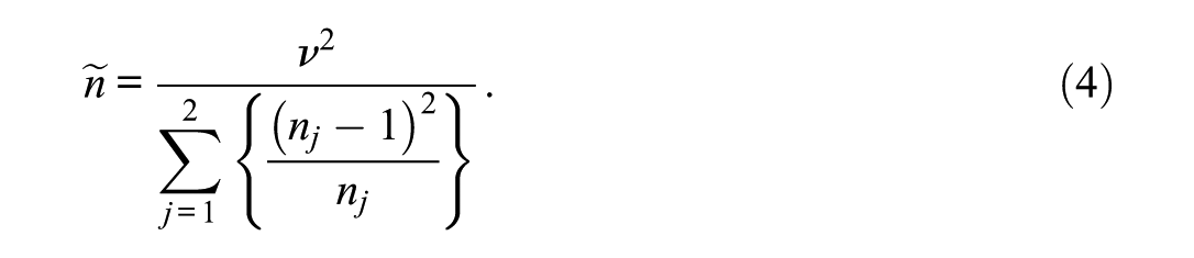
Var (s_{p}^{2}) = \frac{1}{ν^{2}} \sum_{j = 1}^{2} {(n_{j} - 1)}^{2} Var (s_{j}^{2}) = \frac{2 σ^{4}}{ν} + \frac{γ_{2} σ^{4}}{\tilde{n}} .

(3)

where we define the effective sample size for the kurtosis correction:

\tilde{n} = \frac{ν^{2}}{\sum_{j = 1}^{2} {\frac{{(n_{j} - 1)}^{2}}{n_{j}}}} .

(4)

The first term in equation (3) is the variance under normality ( $γ_{2} = 0$ ); the second term is the kurtosis contribution. For balanced designs ( $n_{1} = n_{2} = n$ ), $\tilde{n} = 2 n$ and $ν = 2 (n - 1)$ .

Independence of Numerator and Denominator

A key step in deriving the bias of d is the relationship $E [d] = E [{\bar{X}}_{1} - {\bar{X}}_{2}] \cdot E [s_{p}^{- 1}]$ , which holds exactly only when ${\bar{X}}_{1} - {\bar{X}}_{2}$ and $s_{p}$ are independent. Under normality, this independence follows from Cochran’s theorem. Under nonnormality, independence no longer holds in general, and we must evaluate the resulting error.

Write $d = ({\bar{X}}_{1} - {\bar{X}}_{2}) \cdot s_{p}^{- 1}$ . Then:

E [d] = E [{\bar{X}}_{1} - {\bar{X}}_{2}] \cdot E [s_{p}^{- 1}] + Cov ({\bar{X}}_{1} - {\bar{X}}_{2}, s_{p}^{- 1}) .

(5)

The covariance term can be evaluated using a first-order expansion of $s_{p}^{- 1}$ around $σ^{- 1}$ :

Cov ({\bar{X}}_{1} - {\bar{X}}_{2}, s_{p}^{- 1}) \approx - \frac{1}{2 σ^{3}} Cov ({\bar{X}}_{1} - {\bar{X}}_{2}, s_{p}^{2}) .

Under Assumption A2, $Cov ({\bar{X}}_{j}, s_{j}^{2}) = γ_{1} σ^{3} / n_{j}$ , where $γ_{1}$ is the population skewness (this follows from the joint cumulant $κ_{1, 2} = μ_{3} = γ_{1} σ^{3}$ ). Therefore:

Cov ({\bar{X}}_{1} - {\bar{X}}_{2}, s_{p}^{2}) = \frac{1}{ν} [(n_{1} - 1) \frac{γ_{1} σ^{3}}{n_{1}} - (n_{2} - 1) \frac{γ_{1} σ^{3}}{n_{2}}] .

For balanced designs ( $n_{1} = n_{2}$ ), this expression equals zero regardless of $γ_{1}$ . For unbalanced designs, it is $O (γ_{1} σ^{3} / n)$ , and its contribution to $E [d]$ is

Cov ({\bar{X}}_{1} - {\bar{X}}_{2}, s_{p}^{- 1}) = O (\frac{γ_{1}}{n^{3 / 2}}) .

(6)

Comparing with the kurtosis-induced bias term $3 δ γ_{2} / (8 \tilde{n}) = O (δ γ_{2} / n)$ , the covariance contribution in equation (6) is of lower order ( $O (n^{- 3 / 2})$ vs. $O (n^{- 1})$ ). Therefore, the factorization $E [d] \approx δ σ \cdot E [s_{p}^{- 1}]$ introduces an error that is dominated by the kurtosis-induced bias term for all but extremely skewed distributions with very unbalanced designs. For symmetric distributions ( $γ_{1} = 0$ ), the covariance is exactly zero regardless of sample size balance.

Main Theoretical Result

Proposition 1. Under Assumptions A1–A4, with $n_{1}, n_{2} \to \infty$ such that $n_{1} / n_{2} \to ρ \in (0, \infty)$ and all distributional parameters ( $δ, γ_{1}, γ_{2}, λ_{6}$ ) held fixed, the expectation of Cohen’s d satisfies:

E [d] = δ (1 + \frac{3}{4 ν} + \frac{3 γ_{2}}{8 \tilde{n}}) + R_{n},

(7)

where the remainder $R_{n}$ satisfies:

R_{n} = O (\frac{δ}{n^{2}}) + O (\frac{δ γ_{2}^{2}}{n^{2}}) + O (\frac{γ_{1}}{n^{3 / 2}}) .

(8)

The three terms of $R_{n}$ have distinct origins. The first term, $O (δ / n^{2})$ , arises from the third-order term of the Taylor expansion of $s_{p}^{- 1}$ (Step 1 of the proof below). This term involves $E [{(s_{p}^{2} - σ^{2})}^{3}]$ , the third central moment of the pooled variance; expanding this expectation introduces the sixth central moment of the data (equivalently, the sixth cumulant), which is why Assumption A4 (finite sixth moment) is required to bound it—without a finite sixth moment, $E [{(s_{p}^{2} - σ^{2})}^{3}]$ need not exist, and the $O (n^{- 2})$ order cannot be guaranteed. The second term, $O (δ γ_{2}^{2} / n^{2})$ , arises because the leading kurtosis correction $3 γ_{2} / (8 \tilde{n})$ interacts with itself at second order in the expansion (i.e., the square of a term proportional to $γ_{2} / \tilde{n}$ ), producing a contribution scaled by $γ_{2}^{2}$ ; for the heavy-tailed distributions of interest this term is small relative to the leading $3 δ γ_{2} / (8 \tilde{n})$ correction in equation (7) as long as $γ_{2} / \tilde{n}$ is small. The third term, $O (γ_{1} / n^{3 / 2})$ , is the numerator–denominator covariance (Section “Independence of Numerator and Denominator”), which vanishes for symmetric distributions ( $γ_{1} = 0$ ) or balanced designs ( $n_{1} = n_{2}$ ).

Consequently, the bias of Hedges’ $g = d \cdot J (ν)$ under nonnormality is:

E [g] - δ \approx \frac{3 δ γ_{2}}{8 \tilde{n}} + O (R_{n}) .

(9)

since $J (ν)$ removes the $3 / (4 ν)$ term to $O (ν^{- 2})$ accuracy.

Proof. The proof proceeds in three steps.

Step 1 (Moment expansion of $E [s_{p}^{- 1}]$ ). Let $T = s_{p}^{2}$ with $E [T] = σ^{2}$ . Define $h (t) = t^{- 1 / 2}$ . A Taylor expansion of h around $σ^{2}$ to third order gives, after taking expectations:

h (T) = h (σ^{2}) + h' (σ^{2}) (T - σ^{2}) + \frac{1}{2} h^{″} (σ^{2}) {(T - σ^{2})}^{2} + \frac{1}{6} h'^{″} (σ^{2}) {(T - σ^{2})}^{3} + \dots

where $h' (σ^{2}) = - \frac{1}{2} σ^{- 3}$ , $h^{″} (σ^{2}) = \frac{3}{4} σ^{- 5}$ , $h'^{″} (σ^{2}) = - \frac{15}{8} σ^{- 7}$ .

Taking expectations:

E [s_{p}^{- 1}] = σ^{- 1} + \frac{3}{8 σ^{5}} Var (s_{p}^{2}) - \frac{15}{48 σ^{7}} E [{(s_{p}^{2} - σ^{2})}^{3}] + O (n^{- 2}) .

Substituting equation (3) for $Var (s_{p}^{2})$ :

E [s_{p}^{- 1}] = \frac{1}{σ} (1 + \frac{3}{4 ν} + \frac{3 γ_{2}}{8 \tilde{n}}) + O (\frac{1}{σ n^{2}}) .

The $O (n^{- 2})$ remainder involves $E [{(s_{p}^{2} - σ^{2})}^{3}]$ , which depends on the sixth cumulant of $F_{0}$ (hence Assumption A4).

Step 2 (numerator–denominator factorization). By Section “Independence of Numerator and Denominator”:

E [d] = δ σ \cdot E [s_{p}^{- 1}] + O (γ_{1} n^{- 3 / 2}) .

Step 3 (Combining). Substituting the result of Step 1:

E [d] = δ (1 + \frac{3}{4 ν} + \frac{3 γ_{2}}{8 \tilde{n}}) + R_{n} .

where $R_{n}$ collects the third-order Taylor expansion remainder and the covariance term.

Remark 1 (Role of the sixth moment). Assumption A4 ensures that the third-order term in the Taylor expansion is finite. If only A3 holds (finite fourth moment), the expansion is still valid to second order, but the explicit characterization of the $O (n^{- 2})$ remainder requires the sixth moment. For distributions with extremely heavy tails where the sixth moment may not exist (e.g., $t (ν)$ with $ν \leq 6$ ), the second-order result $E [s_{p}^{- 1}] \approx σ^{- 1} (1 + 3 / (4 ν) + 3 γ_{2} / (8 \tilde{n}))$ remains a useful approximation, but the remainder bound should be interpreted with caution.

Remark 2 (Balanced designs). For balanced designs ( $n_{1} = n_{2}$ ), the covariance term vanishes exactly for any distribution (not only symmetric ones), and the remainder simplifies to $R_{n} = O (δ n^{- 2}) + O (δ γ_{2}^{2} n^{- 2})$ . This makes $g_{κ}^{*}$ particularly well-suited for balanced experimental designs.

Interpretation

The bias of Cohen’s d decomposes into two additive components:

Classical small-sample bias $\approx 3 δ / (4 ν)$ : Present under normality. Removed by Hedges’ $J (ν)$ .

Kurtosis-induced bias $\approx 3 δ γ_{2} / (8 \tilde{n})$ : Present only under nonnormality ( $γ_{2} \neq 0$ ). Not removed by Hedges’ g.

For leptokurtic distributions ( $γ_{2} > 0$ , for example, $t (5)$ with $γ_{2} = 6$ ), the kurtosis-induced bias is positive, making Hedges’ g systematically too large. For platykurtic distributions ( $γ_{2} < 0$ , e.g., Uniform with $γ_{2} = - 1.2$ ), the bias is negative.

The Proposed Estimator

Exact-Anchor Formulation

From Proposition 1, the bias of Hedges’ $g = d \cdot J (ν)$ under nonnormality is approximately $δ \cdot 3 γ_{2} / (8 \tilde{n})$ . To remove this residual bias while preserving the exact Hedges correction under normality, we define:

g_{κ}^{*} = d \cdot \frac{J (ν)}{1 + \frac{3 {\hat{γ}}_{2}}{8 \tilde{n}}} .

(10)

where $J (ν)$ is the exact Hedges correction factor (via the gamma function), and ${\hat{γ}}_{2}$ is the pooled sample excess kurtosis:

{\hat{γ}}_{2} = \frac{\sum_{j = 1}^{2} \sum_{i = 1}^{n_{j}} {(X_{ji} - {\bar{X}}_{j})}^{4}}{{[\sum_{j = 1}^{2} \sum_{i = 1}^{n_{j}} {(X_{ji} - {\bar{X}}_{j})}^{2}]}^{2} / (n_{1} + n_{2})} - 3 .

(11)

where $N = n_{1} + n_{2}$ denotes the total sample size across both groups.

Note that equation (11) defines a biased estimator of $γ_{2}$ , analogous to the natural moment-based formula rather than the bias-corrected k-statistic. We use this form because (a) although its bias is $O (n^{- 1})$ , this bias enters the correction factor only through the term $3 {\hat{γ}}_{2} / (8 \tilde{n})$ , where division by $\tilde{n} = O (n)$ reduces its contribution to the bias of $g_{κ}^{*}$ to $O (n^{- 2})$ —the same order as the remainder $R_{n}$ of Proposition 1 (a formal analysis is given in Section “Plug-in Estimation Error”)—and (b) the pooling structure across two groups makes the k-statistic form unwieldy.

This formulation has a key algebraic property: when ${\hat{γ}}_{2} = 0$ , the denominator equals 1, and $g_{κ}^{*}$ reduces to Hedges’ g. This is algebraically exact. However, under a normal population, ${\hat{γ}}_{2}$ varies around its population value of zero, with small finite-sample bias and sampling variability (variance approximately $24 / N$ ), so $g_{κ}^{*}$ and Hedges’ g will differ slightly in any finite sample from a normal population. The simulation results (Section “Results: Bias”) confirm that these differences are negligible (within Monte Carlo error).

Properties of $g_{κ}^{*}$ :

Algebraic backward compatibility. When ${\hat{γ}}_{2} = 0$ : $g_{κ}^{*} = d \cdot J (ν) = g$ . Under normal populations, $g_{κ}^{*} \approx g$ with negligible finite-sample differences.

Adaptive correction. For ${\hat{γ}}_{2} > 0$ (heavy tails): stronger shrinkage than Hedges’ g. For ${\hat{γ}}_{2} < 0$ (light tails): weaker shrinkage.

Closed-form. No iterative computation or bootstrap required.

Plug-in Estimation Error

The proposed estimator substitutes ${\hat{γ}}_{2}$ for the unknown $γ_{2}$ . This plug-in introduces a secondary source of error that we now quantify.

The pooled sample excess kurtosis ${\hat{γ}}_{2}$ (equation (11)) satisfies $E [{\hat{γ}}_{2}] = γ_{2} + O (n^{- 1})$ , where the $O (n^{- 1})$ term reflects the finite-sample bias of the kurtosis estimator (Joanes & Gill, 1998). The variance of ${\hat{γ}}_{2}$ is:

Var ({\hat{γ}}_{2}) = \frac{24}{N} + \frac{λ_{6} - γ_{2}^{2}}{N} + O (N^{- 2}),

(12)

where $N = n_{1} + n_{2}$ and $λ_{6} = μ_{6} / σ^{6} - 15 - 6 γ_{2}$ involves the sixth moment (cf. Assumption A4). The general large-sample variance of the sample excess kurtosis for a distribution with finite eighth moment is $Var ({\hat{γ}}_{2}) = (μ_{8} / σ^{8} - γ_{2}^{2} - lower - order terms) / N + O (N^{- 2})$ (Stuart & Ord, 1994). Under normality, all cumulants above the second vanish, $μ_{8} / σ^{8} = 105$ , and the expression collapses to the familiar $24 / N$ . Writing the general result as the normal-theory value plus a nonnormality correction yields the two-term form in equation (12): the $24 / N$ term is the normal-theory variance, and $(λ_{6} - γ_{2}^{2}) / N$ is the leading nonnormality adjustment, where $λ_{6}$ collects the sixth-order standardized quantity and $γ_{2}^{2}$ arises because ${\hat{γ}}_{2}$ is itself a function of the (correlated) second and fourth sample moments. For the normal distribution, $λ_{6} = 0$ and $γ_{2} = 0$ , so $Var ({\hat{γ}}_{2}) \approx 24 / N$ .

The plug-in affects the estimator through the factor ${(1 + 3 {\hat{γ}}_{2} / (8 \tilde{n}))}^{- 1}$ . Expanding around $γ_{2}$ :

\frac{1}{1 + \frac{3 {\hat{γ}}_{2}}{8 \tilde{n}}} = \frac{1}{1 + \frac{3 γ_{2}}{8 \tilde{n}}} - \frac{3 / (8 \tilde{n})}{{(1 + \frac{3 γ_{2}}{8 \tilde{n}})}^{2}} ({\hat{γ}}_{2} - γ_{2}) + O (\frac{{({\hat{γ}}_{2} - γ_{2})}^{2}}{{\tilde{n}}^{2}}) .

Taking expectations, the first-order contribution is of order $O (n^{- 2})$ , because $E [{\hat{γ}}_{2} - γ_{2}] = O (n^{- 1})$ and the derivative of the adjustment factor is $O ({\tilde{n}}^{- 1})$ . Thus, the plug-in does not affect the leading-order correction. The second-order term contributes:

E [\frac{{({\hat{γ}}_{2} - γ_{2})}^{2}}{{\tilde{n}}^{2}}] = \frac{Var ({\hat{γ}}_{2})}{{\tilde{n}}^{2}} = O (\frac{1}{N {\tilde{n}}^{2}}) = O (n^{- 3}) .

Therefore, the plug-in estimation error is $O (n^{- 2})$ , which is of the same order as the remainder $R_{n}$ in Proposition 1. In other words, replacing $γ_{2}$ with ${\hat{γ}}_{2}$ does not degrade the accuracy of the bias correction beyond the inherent approximation error of the second-order moment expansion.

Remark 3 (Shrinkage for small samples). Although the plug-in error is theoretically negligible, ${\hat{γ}}_{2}$ can be noisy for $n < 15$ . A practical safeguard is to apply a shrinkage:

{\hat{γ}}_{2}^{(shrink)} = \max (1 - \frac{c}{N}, 0) \cdot {\hat{γ}}_{2},

where $c > 0$ is a tuning constant (e.g., $c = 6$ ). This attenuates the kurtosis correction when N is small, converging to the unshrunken estimator as $N \to \infty$ . In the simulation study (Section “Monte Carlo Simulation Study”), we use the unshrunken ${\hat{γ}}_{2}$ to assess the estimator’s performance without this additional tuning, but we recommend investigating the shrinkage variant in future work.

Variance Estimator and Confidence Interval

For interval estimation, we adopt the standard normal-approximation approach used by Hedges’ g and Bonett (2008). The construction proceeds in two steps. First, we approximate the variance of $g_{κ}^{*}$ via a first-order delta-method argument: treating $J_{κ}^{*} = J (ν) / (1 + 3 {\hat{γ}}_{2} / (8 \tilde{n}))$ as approximately constant (since ${\hat{γ}}_{2} - γ_{2} = O_{p} (n^{- 1 / 2})$ and the derivative of the adjustment factor is $O ({\tilde{n}}^{- 1})$ , so the variation contributes only $O_{p} (n^{- 3 / 2})$ to $g_{κ}^{*}$ ),

Var (g_{κ}^{*}) \approx {(J_{κ}^{*})}^{2} \cdot Var (d) .

Substituting the Bonett (2008) kurtosis-adjusted variance estimator for $Var (d)$ , with $d^{2}$ as a plug-in for $δ^{2}$ :

\hat{Var} (g_{κ}^{*}) = {(\frac{J (ν)}{1 + \frac{3 {\hat{γ}}_{2}}{8 \tilde{n}}})}^{2} (\frac{n_{1} + n_{2}}{n_{1} n_{2}} + \frac{d^{2} ({\hat{γ}}_{2} + 2)}{2 ν}) .

(13)

Second, assuming $g_{κ}^{*}$ is approximately normally distributed in moderate-to-large samples, the $(1 - α)$ confidence interval is:

g_{κ}^{*} \pm z_{α / 2} \sqrt{\hat{Var} (g_{κ}^{*})} .

(14)

Two important caveats apply. First, while Cohen’s d admits a known sampling distribution related to the noncentral t under normality, and is asymptotically normal under broader conditions, we have not formally proven the asymptotic normality of $g_{κ}^{*}$ under nonnormality. Such a result would follow from joint asymptotic normality of $(d, {\hat{γ}}_{2})$ under standard moment conditions, but a formal proof is beyond the scope of this article. The interval (14) should therefore be regarded as a normal-approximation confidence interval whose validity rests on the asymptotic-normality assumption. Second, the variance estimator (13) treats the correction factor as deterministic; ignoring its sampling variability is justified to leading order but contributes a higher-order term to the true variance. The Monte Carlo coverage results in Section “Results: Coverage–Width Trade-off” provide empirical assessment of these approximations across a range of sample sizes and distributions.

Scope of Application

The proposed estimator is designed for primary research where individual participant data (IPD) are available, since computation of ${\hat{γ}}_{2}$ requires access to the raw data (or at minimum, the fourth central moment of each group). In meta-analytic contexts, the estimator can be applied when individual participant data are available (e.g., IPD meta-analysis) or when primary studies report kurtosis. It cannot be applied retrospectively to studies that report only means, standard deviations, and sample sizes. We therefore position $g_{κ}^{*}$ primarily as a tool for primary research, with the recommendation that researchers report ${\hat{γ}}_{2}$ alongside effect sizes to facilitate future meta-analytic use. More broadly, and in line with increasingly standard open-data practice, we encourage researchers to share fully anonymized raw data whenever ethically and legally permissible; doing so enables meta-analysts to compute ${\hat{γ}}_{2}$ (and any other distributional summary) directly, removing the dependence on what the primary study happened to report. Reporting ${\hat{γ}}_{2}$ is thus a minimal fallback for cases where raw-data sharing is not feasible, not a substitute for it.

Comparison of Estimators

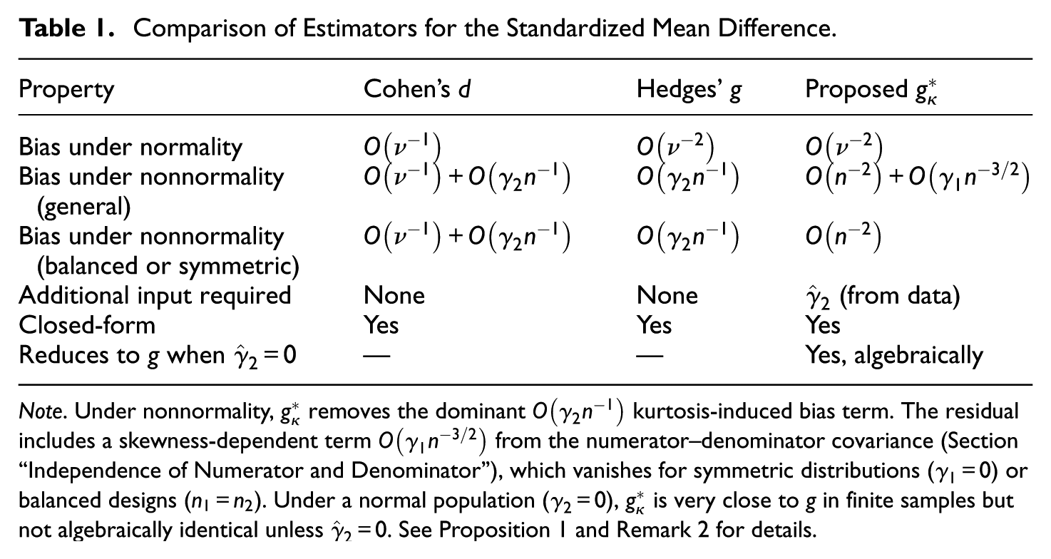
To clarify the position of the proposed estimator relative to existing SMD estimators, Table 1 summarizes the theoretical and practical distinctions among Cohen’s d, Hedges’ g, and the proposed $g_{κ}^{*}$ . The comparison focuses on five features that are central to the present argument: the order of bias under normality, the leading bias term under nonnormality, the additional information required for computation, computational form, and backward compatibility with Hedges’ g. This summary highlights that the proposed estimator does not alter the target estimand or require iterative computation; rather, it retains the conventional SMD framework while removing the leading kurtosis-induced bias term identified in Proposition 1. The table also clarifies the main limitation of the approach: under general nonnormality, residual bias may remain through the skewness-related numerator–denominator covariance term derived in Section “Independence of Numerator and Denominator” (equation (6)), whereas this term vanishes under symmetric distributions or balanced designs.

Table 1.

Comparison of Estimators for the Standardized Mean Difference.

Property	Cohen’s d	Hedges’ g	Proposed $g_{κ}^{*}$
Bias under normality	$O (ν^{- 1})$	$O (ν^{- 2})$	$O (ν^{- 2})$
Bias under nonnormality (general)	$O (ν^{- 1}) + O (γ_{2} n^{- 1})$	$O (γ_{2} n^{- 1})$	$O (n^{- 2}) + O (γ_{1} n^{- 3 / 2})$
Bias under nonnormality (balanced or symmetric)	$O (ν^{- 1}) + O (γ_{2} n^{- 1})$	$O (γ_{2} n^{- 1})$	$O (n^{- 2})$
Additional input required	None	None	${\hat{γ}}_{2}$ (from data)
Closed-form	Yes	Yes	Yes
Reduces to g when ${\hat{γ}}_{2} = 0$	—	—	Yes, algebraically

Note. Under nonnormality, $g_{κ}^{*}$ removes the dominant $O (γ_{2} n^{- 1})$ kurtosis-induced bias term. The residual includes a skewness-dependent term $O (γ_{1} n^{- 3 / 2})$ from the numerator–denominator covariance (Section “Independence of Numerator and Denominator”), which vanishes for symmetric distributions ( $γ_{1} = 0$ ) or balanced designs ( $n_{1} = n_{2}$ ). Under a normal population ( $γ_{2} = 0$ ), $g_{κ}^{*}$ is very close to g in finite samples but not algebraically identical unless ${\hat{γ}}_{2} = 0$ . See Proposition 1 and Remark 2 for details.

Monte Carlo Simulation Study

Design

The simulation employed a fully crossed design with four factors:

(A) Sample size per group ( $n_{1} = n_{2} = n$ ): 10, 15, 20, 30, 50, 100. In addition, three unequal sample size conditions were included: $(n_{1}, n_{2}) \in {(10, 30), (15, 50), (20, 100)}$ .

(b) Population effect size (δ ): 0.0, 0.2, 0.5, 0.8, 1.2, spanning from null to very large effects.

(C) Population distribution: Seven distributions were selected to represent a range of kurtosis values: Normal ( $γ_{2} = 0$ ), $t (10)$ ( $γ_{2} = 1$ ), Lognormal with $σ_{\ln} = 0.5$ ( $γ_{2} \approx 2.4$ ), $χ^{2} (3)$ ( $γ_{2} = 4$ ), $t (5)$ ( $γ_{2} = 6$ ), Exponential ( $γ_{2} = 6$ ), and Uniform ( $γ_{2} = - 1.2$ ). All distributions were standardized to have population mean 0 and variance 1 before applying the location shift δ to Group 1. Note that the $t (5)$ distribution has finite fourth moments but not finite sixth moments, and thus violates Assumption A4 required for Proposition 1. It is included as a stress test to evaluate robustness beyond the formal regularity conditions. All other distributions satisfy Assumptions A1–A4. The standardized densities of all seven distributions, plotted against a standard-normal reference, are shown in the Online Supplement (Figure S1).

This yielded 315 unique conditions for the main simulation. Each condition was replicated $R = 10, 000$ times, for a total of 3,150,000 simulated experiments. An additional 90 conditions for Tukey’s g-and-h distributions (Section “Results: g-and-h Distributions”) and 24 conditions for BCa bootstrap comparison (Section “Results: Comparison With BCa Bootstrap”) were conducted separately. All simulations were conducted in R 4.5.3 with parallel::parLapply for parallelization (seed: 2025). As a supplementary robustness analysis, an additional 18 conditions examined the effect of variance heterogeneity ( $σ_{1}^{2} / σ_{2}^{2} \in {1 : 2, 1 : 4}$ ; Section “Results: Robustness to Variance Heterogeneity”).

Competing Methods

Four interval estimation methods were compared:

(A) Classical Cohen’s d interval: normal-theory variance $\hat{Var} (d) = (n_{1} + n_{2}) / (n_{1} n_{2}) + d^{2} / (2 ν)$ .

(B) Classical Hedges’ g interval: $g \pm z_{α / 2} \sqrt{J {(ν)}^{2} \cdot \hat{Var} (d)}$ .

(C) Proposed $g_{κ}^{*}$ interval: Equation (14), which adjusts both the point estimate and the variance estimator for kurtosis.

(D) Bonett (2008) interval: Hedges’ g point estimate with kurtosis-adjusted variance ${\hat{Var}}_{Bonett} (g) = J {(ν)}^{2} [(n_{1} + n_{2}) / (n_{1} n_{2}) + d^{2} ({\hat{γ}}_{2} + 2) / (2 ν)]$ .

The Bonett method modifies only the variance estimator, not the point estimate, and thus provides a natural comparator: it isolates the contribution of the kurtosis-adjusted point estimate (unique to our proposal) from the kurtosis-adjusted variance estimate (shared by both methods).

Evaluation Criteria

Four criteria were used: (a) bias, (b) mean squared error (MSE), (c) 95% CI coverage probability, and (d) CI width. We assess coverage and width jointly (Section “Results: Coverage–Width Trade-off”) but do not combine them into a single index. The Monte Carlo standard error of the coverage estimate is $\sqrt{0.95 \times 0.05 / 10, 000} \approx 0.002$ , so deviations from the nominal .950 exceeding approximately 0.006 (three SE) are considered noteworthy.

Results: Bias

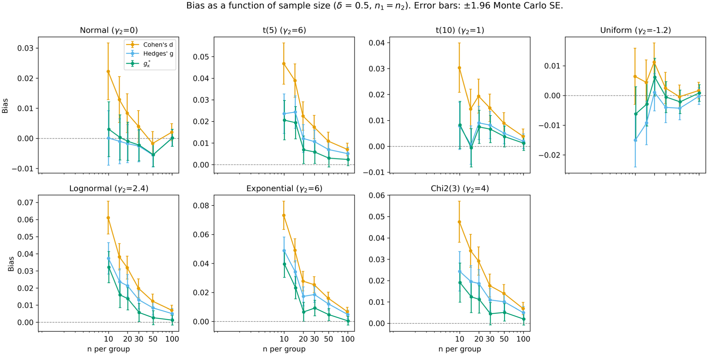
Figure 1 shows the bias of each point estimator as a function of sample size for $δ = 0.5$ .

Figure 1.

Bias as a function of sample size ( $δ = 0.5$ , $n_{1} = n_{2}$ ).

Three patterns are evident. First, under normality, the theoretical bias of Hedges’ g is exactly zero. The small fluctuations of g and $g_{κ}^{*}$ around zero in Figure 1 reflect Monte Carlo sampling variability (MC SE ≈.002), not systematic bias. In contrast, Cohen’s d shows a systematic positive bias that decreases with sample size.

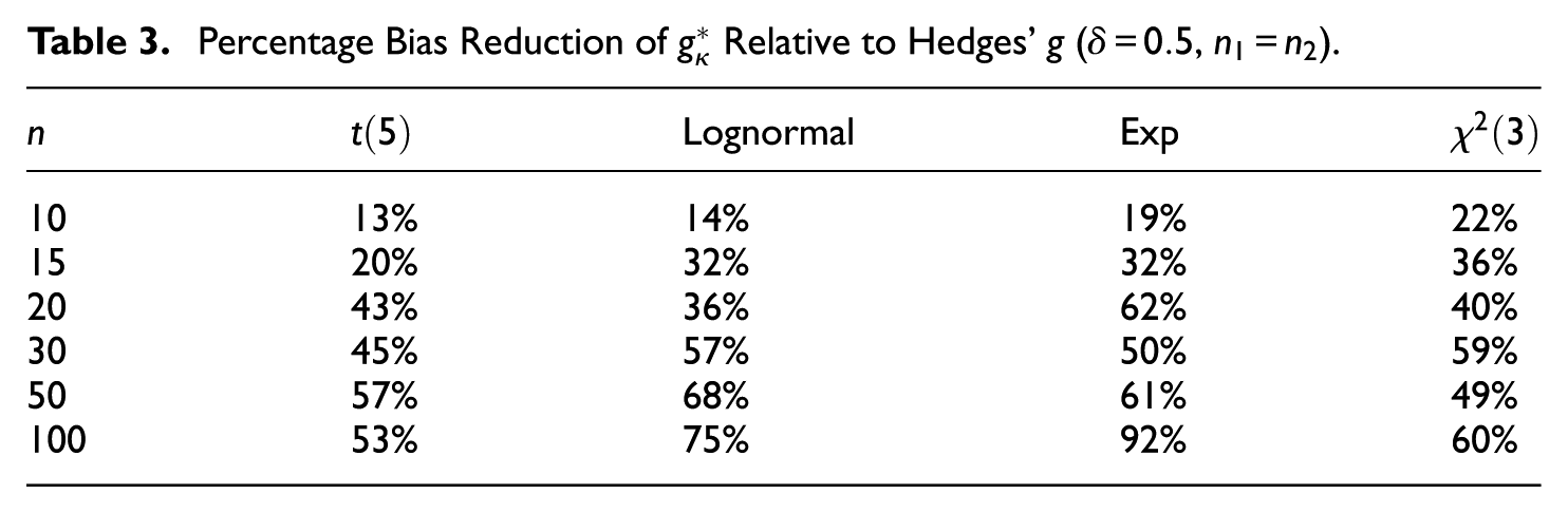
Second, under heavy-tailed distributions, $g_{κ}^{*}$ substantially reduces the residual bias of Hedges’ g. For example, under $t (5)$ at $n = 50$ , the bias of g is 0.0070 compared with 0.0030 for $g_{κ}^{*}$ (57% reduction). Under the exponential distribution at $n = 100$ , the reduction reaches 92% (from 0.0048 to 0.0004). Under the lognormal distribution at $n = 50$ , it is 68% (from 0.0084 to 0.0027).

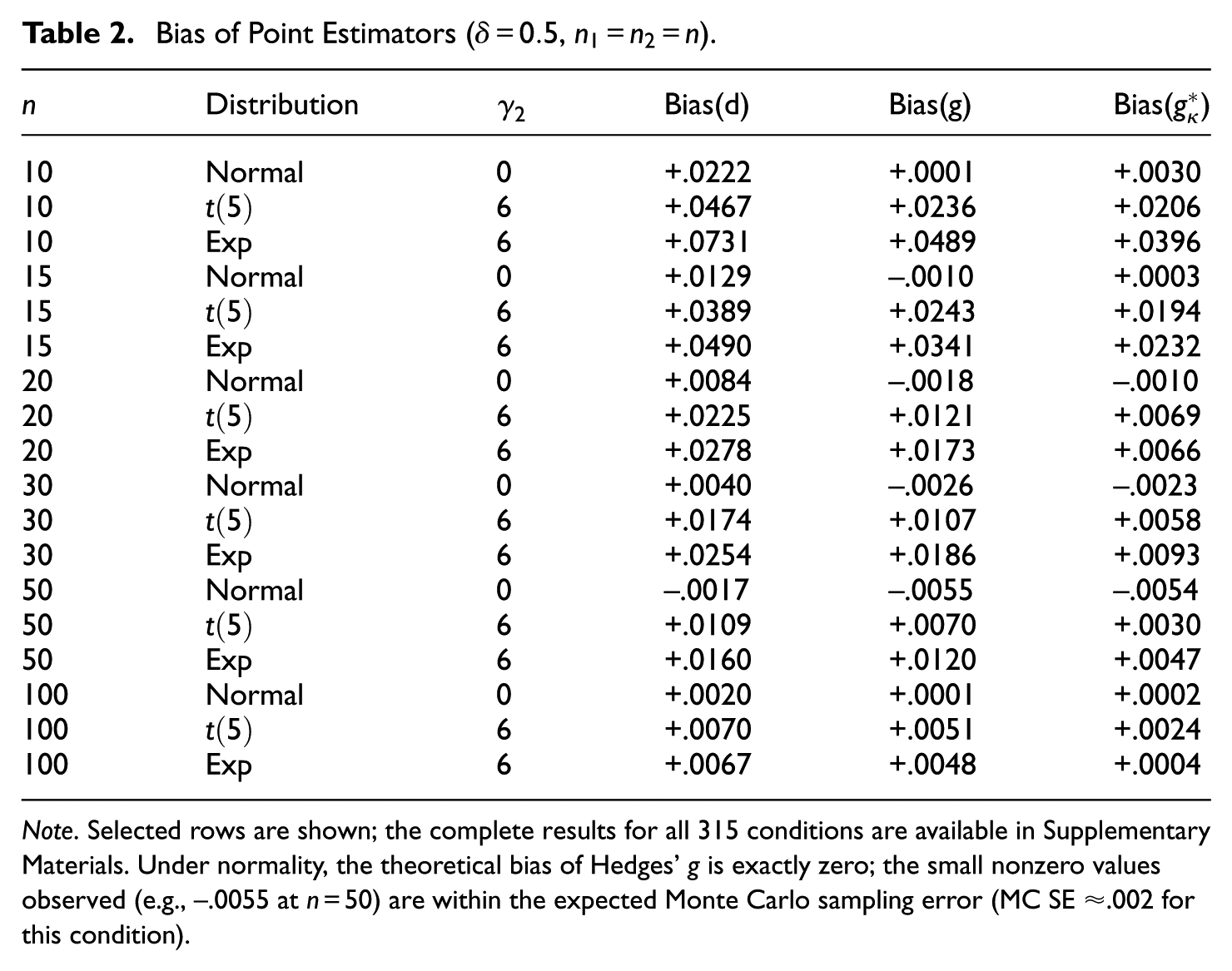
Third, under the uniform distribution ( $γ_{2} = - 1.2$ ), Hedges’ g shows a slight overcorrection (negative bias at small n), while $g_{κ}^{*}$ brings the bias closer to zero. Table 2 reports representative numerical values underlying these patterns.

Table 2.

Bias of Point Estimators ( $δ = 0.5$ , $n_{1} = n_{2} = n$ ).

n	Distribution	$γ_{2}$	Bias(d)	Bias(g)	Bias( $g_{κ}^{*}$ )
10	Normal	0	+.0222	+.0001	+.0030
10	$t (5)$	6	+.0467	+.0236	+.0206
10	Exp	6	+.0731	+.0489	+.0396
15	Normal	0	+.0129	−.0010	+.0003
15	$t (5)$	6	+.0389	+.0243	+.0194
15	Exp	6	+.0490	+.0341	+.0232
20	Normal	0	+.0084	−.0018	−.0010
20	$t (5)$	6	+.0225	+.0121	+.0069
20	Exp	6	+.0278	+.0173	+.0066
30	Normal	0	+.0040	−.0026	−.0023
30	$t (5)$	6	+.0174	+.0107	+.0058
30	Exp	6	+.0254	+.0186	+.0093
50	Normal	0	−.0017	−.0055	−.0054
50	$t (5)$	6	+.0109	+.0070	+.0030
50	Exp	6	+.0160	+.0120	+.0047
100	Normal	0	+.0020	+.0001	+.0002
100	$t (5)$	6	+.0070	+.0051	+.0024
100	Exp	6	+.0067	+.0048	+.0004

Note. Selected rows are shown; the complete results for all 315 conditions are available in Supplementary Materials. Under normality, the theoretical bias of Hedges’ g is exactly zero; the small nonzero values observed (e.g., −.0055 at $n = 50$ ) are within the expected Monte Carlo sampling error (MC SE ≈.002 for this condition).

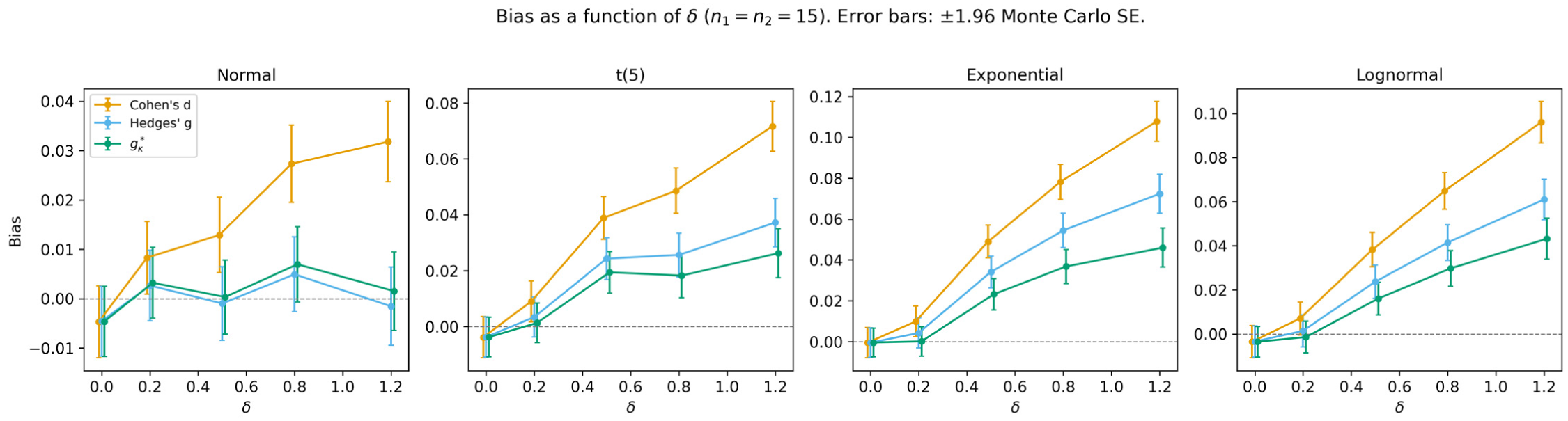
Figure 2 shows that the bias scales approximately linearly with δ, consistent with Proposition 1.

Figure 2.

Bias as a function of δ ( $n_{1} = n_{2} = 15$ ).

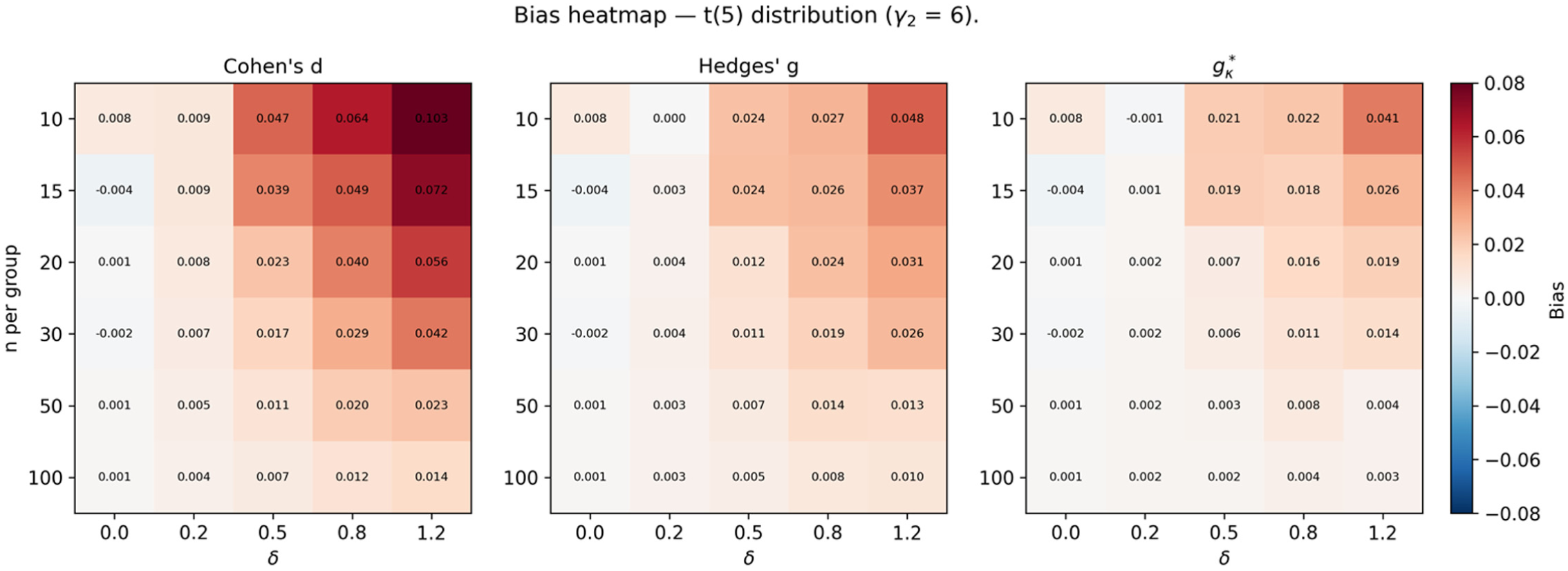
Figure 3 provides a heatmap visualization of the bias under the $t (5)$ distribution across all sample sizes and effect sizes, showing the advantage of $g_{κ}^{*}$ throughout the parameter space.

Figure 3.

Bias heatmap — $t (5)$ distribution ( $γ_{2} = 6$ ).

Table 3 summarizes the bias reduction percentage for key conditions.

Table 3.

Percentage Bias Reduction of $g_{κ}^{*}$ Relative to Hedges’ g ( $δ = 0.5$ , $n_{1} = n_{2}$ ).

n	$t (5)$	Lognormal	Exp	$χ^{2} (3)$
10	13%	14%	19%	22%
15	20%	32%	32%	36%
20	43%	36%	62%	40%
30	45%	57%	50%	59%
50	57%	68%	61%	49%
100	53%	75%	92%	60%

Results: MSE and Relative Efficiency

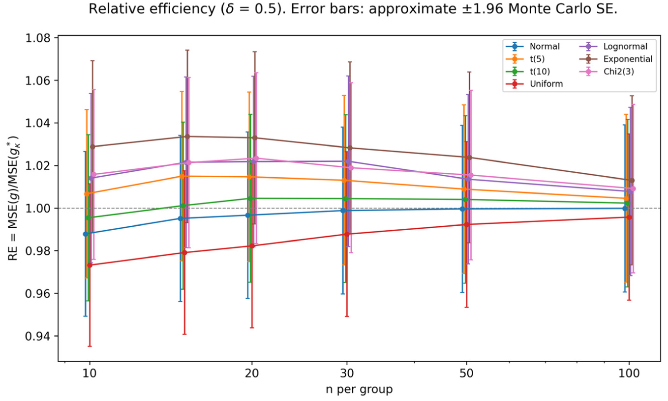
Figure 4 shows the relative efficiency $RE = MSE (g) / MSE (g_{κ}^{*})$ . Values above 1.0 indicate that $g_{κ}^{*}$ is more efficient. Under normality, RE remains close to 1.0 (range: 0.998–1.005), confirming negligible efficiency loss. Under heavy-tailed distributions, RE exceeds 1.0 (typical range: 1.00–1.03), indicating that $g_{κ}^{*}$ matches or modestly exceeds Hedges’ g in MSE.

Figure 4.

Relative efficiency $MSE (g) / MSE (g_{κ}^{*})$ ( $δ = 0.5$ ).

This addresses the bias–variance trade-off explicitly. The kurtosis correction reduces bias substantially (36%–92% under heavy-tailed conditions), while the variance of $g_{κ}^{*}$ is essentially the same as that of g (since the multiplicative correction factor is $1 + O_{p} (n^{- 1 / 2})$ , applying it leaves the variance to leading order unchanged). Consequently, the bias reduction translates directly into MSE reduction, with no penalty on the variance side. In other words, despite our principal focus on bias (Section “Scope: The Class of Distributions Addressed”), the proposed estimator does not sacrifice variance efficiency relative to Hedges’ g under any of the conditions examined.

Results: Coverage–Width Trade-off

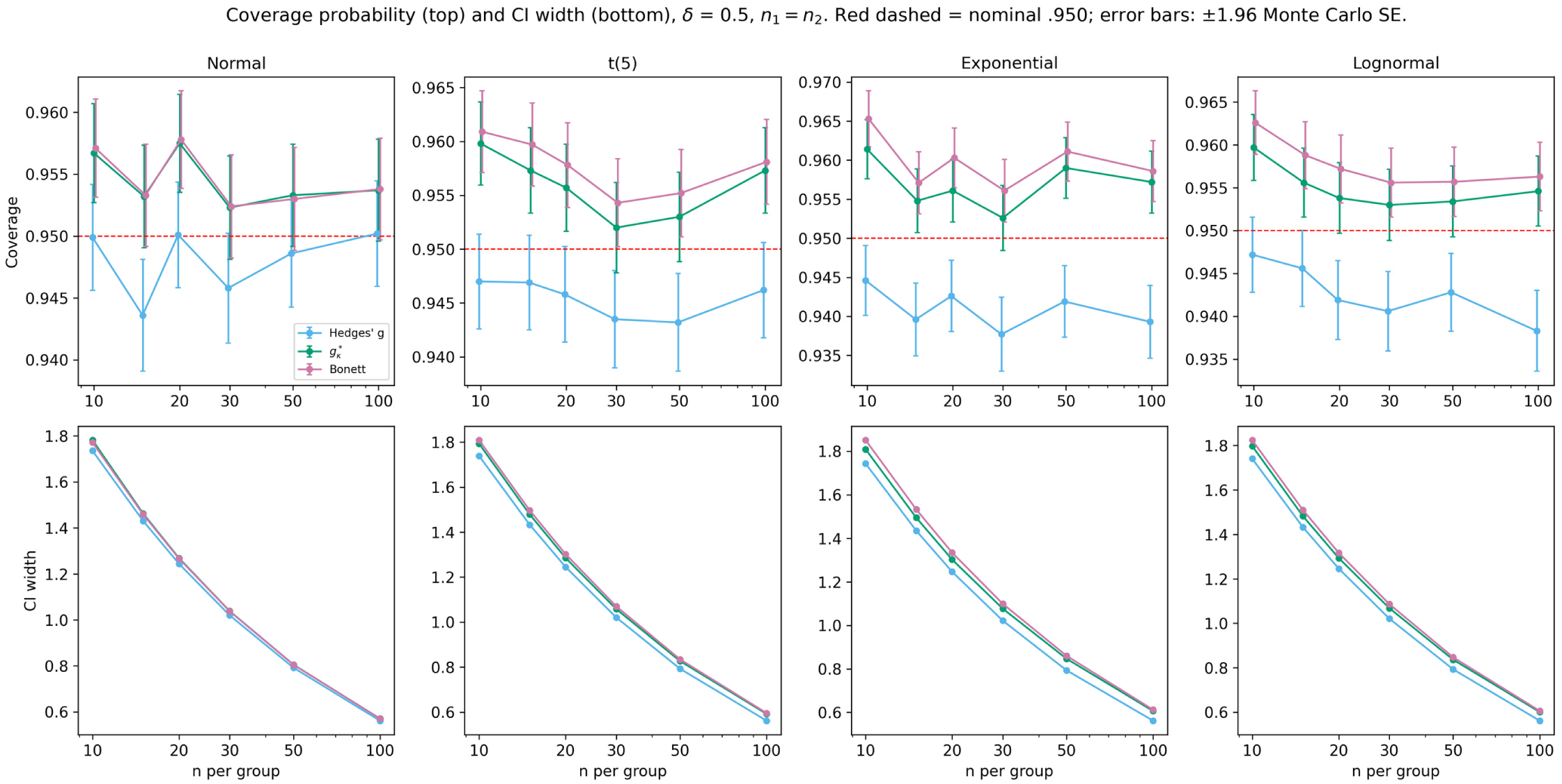
Figure 5 presents both coverage probability (top panels) and CI width (bottom panels) side by side, directly addressing the question of whether improved coverage comes at the cost of wider intervals.

Figure 5.

Coverage probability (top) and CI width (bottom), $δ = 0.5$ , $n_{1} = n_{2}$ .

Under normality, the three interval methods shown in Figure 5 (Hedges’ g, $g_{κ}^{*}$ , and Bonett) achieve coverage close to .950 with similar widths; the classical Cohen’s d interval (not plotted) behaves similarly. Under nonnormal distributions, two patterns emerge.

First, the classical intervals (d and g) show persistent undercoverage. Across the heavy-tailed distributions ( $t (5)$ , Exponential, Lognormal) at $δ = 0.5$ , coverage of the Hedges’ g interval ranged from .938 to .947, consistently below the nominal .950 level.

Second, both $g_{κ}^{*}$ and Bonett achieve coverage closer to .950. Across the same conditions, coverage of $g_{κ}^{*}$ ranged from .952 to .961, and Bonett from .954 to .961. The improvement comes with a modest increase in CI width.

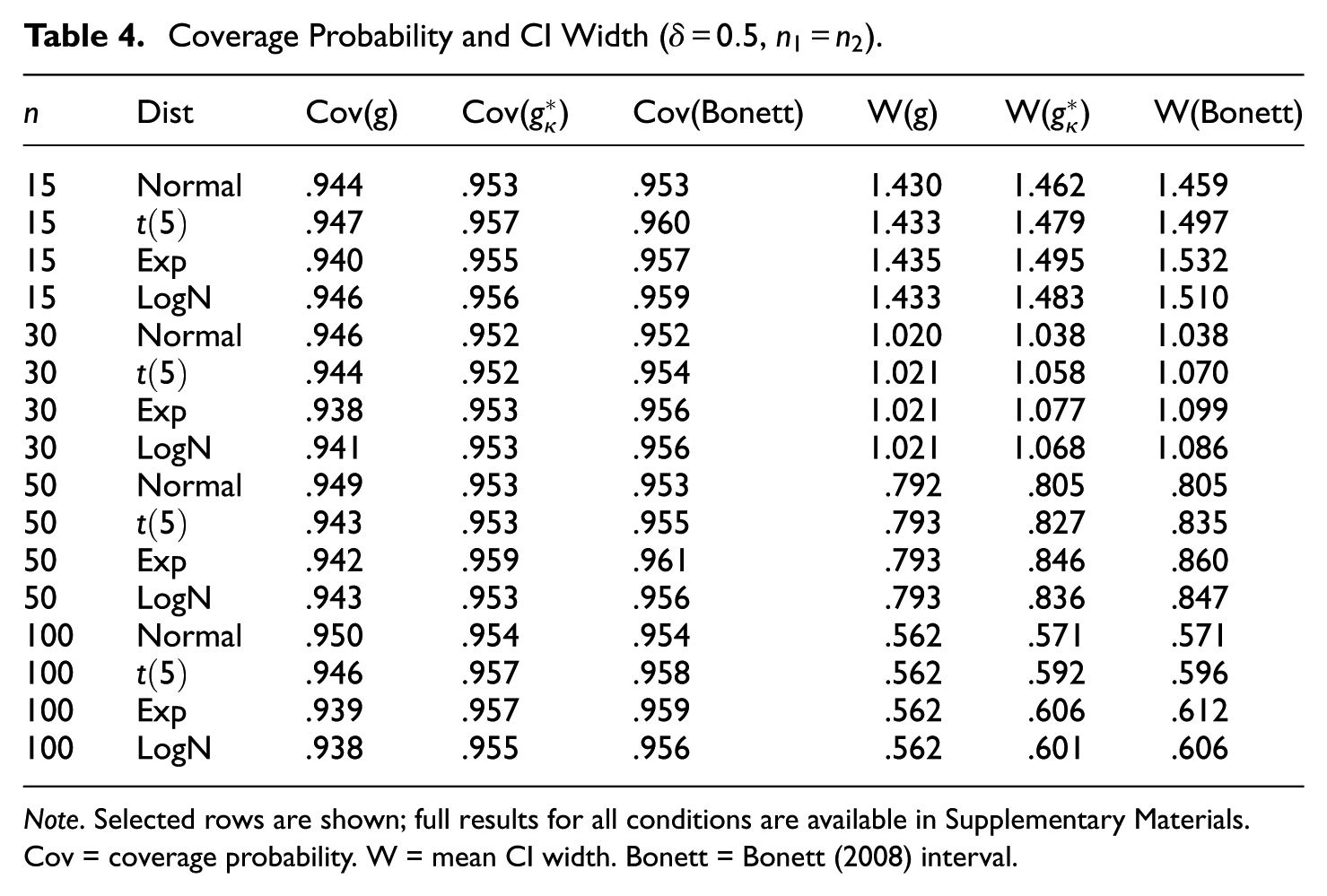
Critically, the width increase is proportionate. For example, under the exponential distribution at $n = 50$ , the g interval has width 0.793 and coverage .942, while the $g_{κ}^{*}$ interval has width 0.846 (+6.7%) and coverage .959. The Bonett interval achieves coverage .961 with width 0.860 (+8.4%). Thus, $g_{κ}^{*}$ achieves comparable coverage to Bonett with consistently narrower intervals, because the point estimate correction reduces the bias component of the coverage error, allowing the variance component to “do less work.”Table 4 lists the coverage probabilities and interval widths for representative conditions.

Table 4.

Coverage Probability and CI Width ( $δ = 0.5$ , $n_{1} = n_{2}$ ).

n	Dist	Cov(g)	Cov( $g_{κ}^{*}$ )	Cov(Bonett)	W(g)	W( $g_{κ}^{*}$ )	W(Bonett)
15	Normal	.944	.953	.953	1.430	1.462	1.459
15	$t (5)$	.947	.957	.960	1.433	1.479	1.497
15	Exp	.940	.955	.957	1.435	1.495	1.532
15	LogN	.946	.956	.959	1.433	1.483	1.510
30	Normal	.946	.952	.952	1.020	1.038	1.038
30	$t (5)$	.944	.952	.954	1.021	1.058	1.070
30	Exp	.938	.953	.956	1.021	1.077	1.099
30	LogN	.941	.953	.956	1.021	1.068	1.086
50	Normal	.949	.953	.953	.792	.805	.805
50	$t (5)$	.943	.953	.955	.793	.827	.835
50	Exp	.942	.959	.961	.793	.846	.860
50	LogN	.943	.953	.956	.793	.836	.847
100	Normal	.950	.954	.954	.562	.571	.571
100	$t (5)$	.946	.957	.958	.562	.592	.596
100	Exp	.939	.957	.959	.562	.606	.612
100	LogN	.938	.955	.956	.562	.601	.606

Note. Selected rows are shown; full results for all conditions are available in Supplementary Materials. Cov = coverage probability. W = mean CI width. Bonett = Bonett (2008) interval.

Results: Unequal Sample Sizes

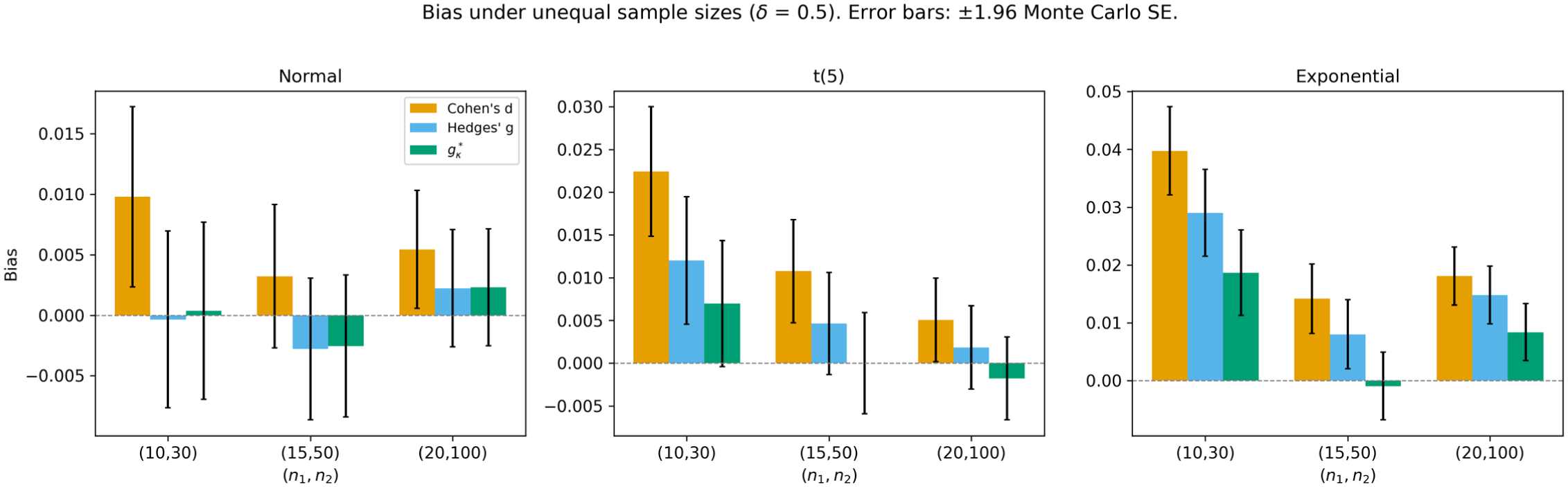
Figure 6 shows the bias under unequal sample size conditions at $δ = 0.5$ . The effective sample size $\tilde{n}$ (equation (4)) appropriately weights each group’s contribution. Under the $t (5)$ distribution with $(n_{1}, n_{2}) = (15, 50)$ , the bias of Hedges’ g is 0.0047 compared with approximately 0 for $g_{κ}^{*}$ . Coverage also improves: under the exponential distribution with $(10, 30)$ , coverage of g is .946 compared with .963 for $g_{κ}^{*}$ . The complete results for all unequal-sample-size conditions are provided in the Online Supplement (Table S1); Table 4 reports balanced designs only.

Figure 6.

Bias under unequal sample sizes ( $δ = 0.5$ ).

Results: g-and-h Distributions

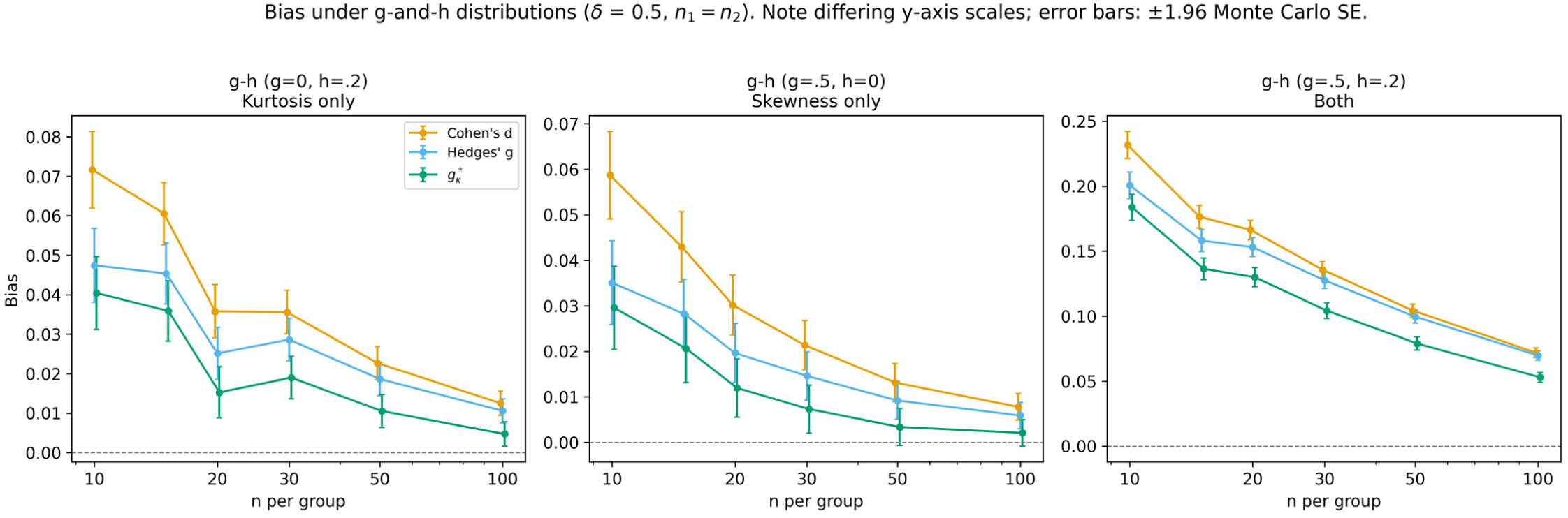
To independently assess the roles of skewness and kurtosis, we examined three distributions from Tukey’s g-and-h family (Hoaglin, 1985): ( $g = 0, h = 0.2$ ) for symmetric heavy tails (kurtosis only), ( $g = 0.5, h = 0$ ) for skewed light tails (skewness only), and ( $g = 0.5, h = 0.2$ ) for skewed heavy tails (both). Population-level standardization constants were estimated via Monte Carlo ( $10^{6}$ draws) to avoid the artifact of within-sample standardization. Because the rth moment of a g-and-h variable exists only when $hr < 1$ , distributions with $h = 0.2$ lack finite sixth moments ( $0.2 \times 6 = 1.2 > 1$ ) and thus violate Assumption A4. These conditions should therefore be interpreted as supplementary boundary-case stress tests rather than direct confirmations of Proposition 1. The standardized densities of the three g-and-h distributions are shown in the Online Supplement (Figure S2).

Figure 7 presents the bias under these three conditions for $δ = 0.5$ . Three informative patterns emerge.

Figure 7.

Bias under g-and-h distributions ( $δ = 0.5$ , $n_{1} = n_{2}$ ).

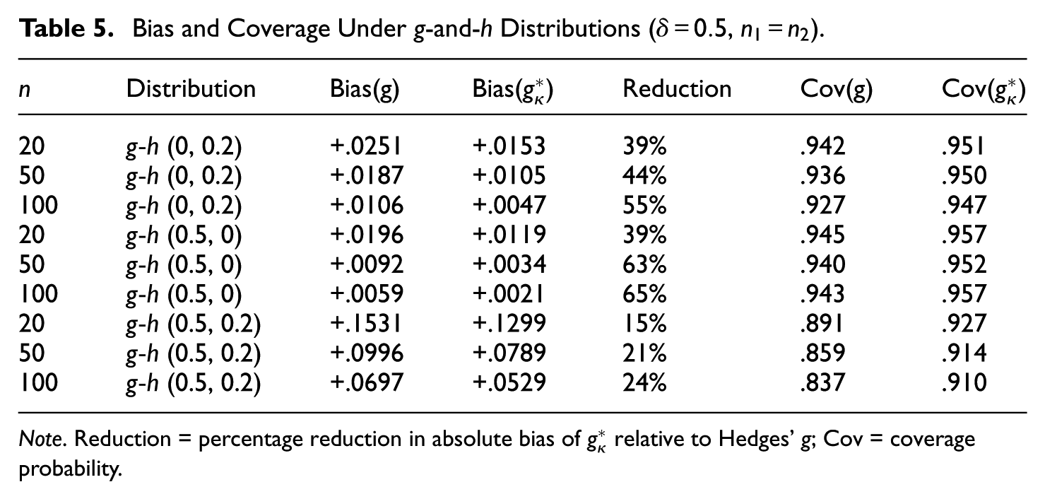
First, under the ( $g = 0, h = 0.2$ ) distribution (symmetric, heavy-tailed), $g_{κ}^{*}$ reduced the bias of Hedges’ g by 34%–55% at $n \geq 20$ , confirming that the kurtosis correction works as intended when kurtosis is the dominant source of nonnormality.

Second, under the ( $g = 0.5, h = 0$ ) distribution (skewed, no h-induced kurtosis), $g_{κ}^{*}$ also achieved substantial bias reduction (39%–65% at $n \geq 20$ ). This initially appears surprising since the correction is designed to address kurtosis, not skewness. However, the g transformation itself generates excess kurtosis: at $n = 100$ , ${\hat{γ}}_{2} \approx 4.3$ . The kurtosis correction appropriately detects and adjusts for this indirectly generated kurtosis, regardless of its source.

Third, under the ( $g = 0.5, h = 0.2$ ) distribution (both skewness and heavy tails), the bias was substantially larger than in the other two conditions (bias of g = 0.070–0.200), and $g_{κ}^{*}$ achieved only 15% to 24% reduction. The estimated kurtosis was very high ( ${\hat{γ}}_{2} = 8$ –21), but the extreme skewness creates additional bias through the numerator–denominator covariance channel (Section “Independence of Numerator and Denominator”) that the kurtosis correction alone cannot address. This result delineates the boundary of the proposed correction: when both severe skewness ( $γ_{1} > 2$ ) and extreme kurtosis ( $γ_{2} > 10$ ) are present simultaneously, $g_{κ}^{*}$ still improves over Hedges’ g but does not fully remove the bias. Table 5 reports the corresponding bias, percentage reduction, and coverage for the three g-and-h conditions.

Table 5.

Bias and Coverage Under g-and-h Distributions ( $δ = 0.5$ , $n_{1} = n_{2}$ ).

n	Distribution	Bias(g)	Bias( $g_{κ}^{*}$ )	Reduction	Cov(g)	Cov( $g_{κ}^{*}$ )
20	g-h (0, 0.2)	+.0251	+.0153	39%	.942	.951
50	g-h (0, 0.2)	+.0187	+.0105	44%	.936	.950
100	g-h (0, 0.2)	+.0106	+.0047	55%	.927	.947
20	g-h (0.5, 0)	+.0196	+.0119	39%	.945	.957
50	g-h (0.5, 0)	+.0092	+.0034	63%	.940	.952
100	g-h (0.5, 0)	+.0059	+.0021	65%	.943	.957
20	g-h (0.5, 0.2)	+.1531	+.1299	15%	.891	.927
50	g-h (0.5, 0.2)	+.0996	+.0789	21%	.859	.914
100	g-h (0.5, 0.2)	+.0697	+.0529	24%	.837	.910

Note. Reduction = percentage reduction in absolute bias of $g_{κ}^{*}$ relative to Hedges’ g; Cov = coverage probability.

Results: Comparison With BCa Bootstrap

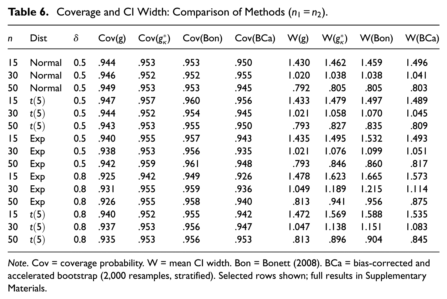
To compare $g_{κ}^{*}$ with a resampling-based approach, we computed BCa (bias-corrected and accelerated) bootstrap confidence intervals (Efron & Tibshirani, 1993) for Hedges’ g across 24 selected conditions (3 sample sizes × 2 effect sizes × 4 distributions, 2,000 replications × 2,000 stratified bootstrap resamples each). Resampling was conducted within each group to preserve the two-sample structure (stratified bootstrap). The computation was successful in all 48,000 replications (0% failure rate), with only 14 instances (0.03%) producing the norm.inter endpoint warning. This warning is issued by the boot package’s boot.ci function when a BCa interval endpoint falls at or beyond the most extreme order statistic of the bootstrap distribution, so that the endpoint is obtained by extrapolation rather than by interpolation between adjacent order statistics. Because the warning affected only 0.03% of replications and indicates mild extrapolation rather than computational failure, we retained these replications; recomputing coverage with them excluded changed the reported values by less than .001 in every condition.

Table 6 presents the comparison. At $δ = 0.5$ , BCa coverage for nonnormal distributions ranged from .935 to .956, compared with .952–.959 for $g_{κ}^{*}$ and .954–.961 for Bonett. BCa interval widths were slightly narrower than $g_{κ}^{*}$ in most conditions (mean width 1.116 vs. 1.123), but this narrower width came with lower coverage. At $δ = 0.8$ , the differences were more pronounced: BCa coverage for nonnormal distributions ranged from .926 to .953, while $g_{κ}^{*}$ maintained .942–.955.

Table 6.

Coverage and CI Width: Comparison of Methods ( $n_{1} = n_{2}$ ).

n	Dist	δ	Cov(g)	Cov( $g_{κ}^{*}$ )	Cov(Bon)	Cov(BCa)	W(g)	W( $g_{κ}^{*}$ )	W(Bon)	W(BCa)
15	Normal	0.5	.944	.953	.953	.950	1.430	1.462	1.459	1.496
30	Normal	0.5	.946	.952	.952	.955	1.020	1.038	1.038	1.041
50	Normal	0.5	.949	.953	.953	.945	.792	.805	.805	.803
15	$t (5)$	0.5	.947	.957	.960	.956	1.433	1.479	1.497	1.489
30	$t (5)$	0.5	.944	.952	.954	.945	1.021	1.058	1.070	1.045
50	$t (5)$	0.5	.943	.953	.955	.950	.793	.827	.835	.809
15	Exp	0.5	.940	.955	.957	.943	1.435	1.495	1.532	1.493
30	Exp	0.5	.938	.953	.956	.935	1.021	1.076	1.099	1.051
50	Exp	0.5	.942	.959	.961	.948	.793	.846	.860	.817
15	Exp	0.8	.925	.942	.949	.926	1.478	1.623	1.665	1.573
30	Exp	0.8	.931	.955	.959	.936	1.049	1.189	1.215	1.114
50	Exp	0.8	.926	.955	.958	.940	.813	.941	.956	.875
15	$t (5)$	0.8	.940	.952	.955	.942	1.472	1.569	1.588	1.535
30	$t (5)$	0.8	.937	.953	.956	.947	1.047	1.138	1.151	1.083
50	$t (5)$	0.8	.935	.953	.956	.953	.813	.896	.904	.845

Note. Cov = coverage probability. W = mean CI width. Bon = Bonett (2008). BCa = bias-corrected and accelerated bootstrap (2,000 resamples, stratified). Selected rows shown; full results in Supplementary Materials.

The comparison reveals a fundamental trade-off. BCa is a nonparametric method that makes no distributional assumptions, while $g_{κ}^{*}$ exploits the parametric structure of the kurtosis correction. The parametric approach achieves more consistent coverage under the conditions examined, particularly when δ is moderate-to-large and the distribution is heavy-tailed. A practical advantage of $g_{κ}^{*}$ is computational efficiency: BCa requires $B \times R$ resamples (here, $2, 000 \times 2, 000 = 4 \times 10^{6}$ per condition), whereas $g_{κ}^{*}$ is computed in closed form.

Results: Robustness to Variance Heterogeneity

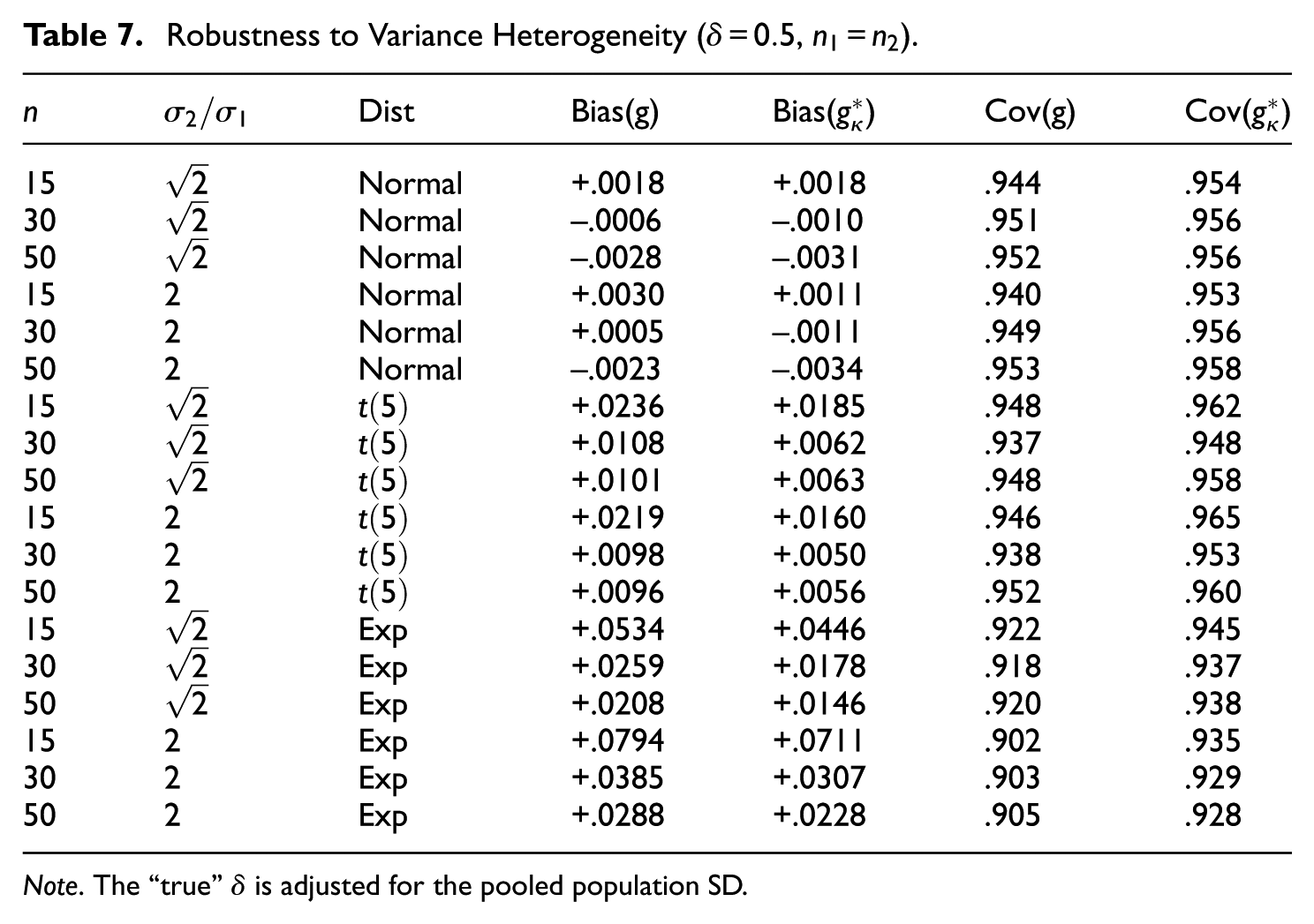
Although Assumption A2 requires equal population variances, we examined the robustness of $g_{κ}^{*}$ under moderate violations. Table 7 presents bias and coverage when Group 2 has a larger standard deviation ( $σ_{2} / σ_{1} \in {\sqrt{2}, 2}$ , corresponding to variance ratios of 1:2 and 1:4), with balanced sample sizes and $δ = 0.5$ .

Table 7.

Robustness to Variance Heterogeneity ( $δ = 0.5$ , $n_{1} = n_{2}$ ).

n	$σ_{2} / σ_{1}$	Dist	Bias(g)	Bias( $g_{κ}^{*}$ )	Cov(g)	Cov( $g_{κ}^{*}$ )
15	$\sqrt{2}$	Normal	+.0018	+.0018	.944	.954
30	$\sqrt{2}$	Normal	−.0006	−.0010	.951	.956
50	$\sqrt{2}$	Normal	−.0028	−.0031	.952	.956
15	2	Normal	+.0030	+.0011	.940	.953
30	2	Normal	+.0005	−.0011	.949	.956
50	2	Normal	−.0023	−.0034	.953	.958
15	$\sqrt{2}$	$t (5)$	+.0236	+.0185	.948	.962
30	$\sqrt{2}$	$t (5)$	+.0108	+.0062	.937	.948
50	$\sqrt{2}$	$t (5)$	+.0101	+.0063	.948	.958
15	2	$t (5)$	+.0219	+.0160	.946	.965
30	2	$t (5)$	+.0098	+.0050	.938	.953
50	2	$t (5)$	+.0096	+.0056	.952	.960
15	$\sqrt{2}$	Exp	+.0534	+.0446	.922	.945
30	$\sqrt{2}$	Exp	+.0259	+.0178	.918	.937
50	$\sqrt{2}$	Exp	+.0208	+.0146	.920	.938
15	2	Exp	+.0794	+.0711	.902	.935
30	2	Exp	+.0385	+.0307	.903	.929
50	2	Exp	+.0288	+.0228	.905	.928

Note. The “true”δ is adjusted for the pooled population SD.

The results differ by distribution. For the normal distribution—where there is no excess kurtosis to correct— $g_{κ}^{*}$ and Hedges’ g have essentially identical bias; the small differences observed (e.g., $- . 0010$ vs. $- . 0006$ at $n = 30$ , $σ_{2} / σ_{1} = \sqrt{2}$ ) are within Monte Carlo error and can favor either estimator. For the leptokurtic distributions ( $t (5)$ , Exponential), $g_{κ}^{*}$ reduces bias relative to Hedges’ g across the heterogeneity conditions examined, and its coverage is closer to nominal in nearly all cells. Thus, the bias advantage of $g_{κ}^{*}$ under variance heterogeneity is specific to the heavy-tailed cases for which the kurtosis correction is designed; under normality, the two estimators are interchangeable. However, under the exponential distribution with $σ_{2} / σ_{1} = 2$ , coverage of $g_{κ}^{*}$ falls to .928–.935, well below the nominal .950, indicating that the kurtosis correction alone cannot overcome the combined effects of severe nonnormality and substantial variance heterogeneity. This underscores the importance of Assumption A2 and motivates future work on heteroscedastic extensions.

Illustrative Application

Prevalence of Nonnormality in Practice

Before presenting numerical examples, we situate the practical relevance of $g_{κ}^{*}$ in the context of real data. Blanca et al. (2013) analyzed the distributional shapes of 693 variables from 404 psychological and educational studies. They found that the modal excess kurtosis was between 0 and 1, but that a substantial proportion of variables exhibited moderate-to-high kurtosis: 34.7% had $γ_{2} > 1$ , 17.4% had $γ_{2} > 2$ , and distributions with $γ_{2} > 6$ (e.g., reaction time data, clinical symptom counts) were not uncommon. These findings indicate that the kurtosis correction provided by $g_{κ}^{*}$ is relevant to a meaningful portion of empirical research.

Empirical Baseline: Near-Normal Data

To confirm that $g_{κ}^{*}$ imposes no unnecessary adjustment when data are approximately normal, we analyzed a publicly available educational data set (Royce Kimmons, “Students Performance in Exams”; $N = 1, 000$ ). Comparing writing scores between students who completed a test preparation course ( $n_{1} = 358$ , $M = 74.4$ , $SD = 13.4$ ) and those who did not ( $n_{2} = 642$ , $M = 64.5$ , $SD = 15.0$ ), the pooled excess kurtosis was ${\hat{γ}}_{2} = 0.034$ . As expected, the three estimators were essentially identical: Cohen’s $d = 0.687$ , Hedges’ $g = 0.686$ , $g_{κ}^{*} = 0.686$ . The kurtosis correction factor was $1 / (1 + 3 \times 0.034 / (8 \times 999)) = 0.999987$ , confirming that the adjustment is negligible for near-normal data.

Real Data With Mild Leptokurtosis

We next applied $g_{κ}^{*}$ to data from a Stroop task experiment (Lakens, 2014; data available at https://github.com/Lakens/Stroop). Students in an introductory psychology course completed an online Stroop task in two cohorts (2013: $n = 83$ ; 2014: $n = 48$ ). We compared congruent-trial completion times between cohorts as an independent two-group comparison.

The 2013 cohort exhibited mild positive skewness ( ${\hat{γ}}_{1} = 0.89$ ) and moderate leptokurtosis ( ${\hat{γ}}_{2} = 1.65$ ), characteristic of response time data. The 2014 cohort was more symmetric ( ${\hat{γ}}_{1} = 0.23$ , ${\hat{γ}}_{2} = - 0.58$ ). The pooled excess kurtosis was ${\hat{γ}}_{2} = 1.22$ .

The effect sizes were: Cohen’s $d = - 0.094$ , Hedges’ $g = - 0.094$ , $g_{κ}^{*} = - 0.093$ . The difference of 0.0003 between g and $g_{κ}^{*}$ is small for two reasons: (a) the kurtosis is moderate ( ${\hat{γ}}_{2} = 1.2$ ) and (b) the total sample is relatively large ( $N = 131$ ), so $3 {\hat{γ}}_{2} / (8 \tilde{n})$ is small. This example illustrates a common scenario in practice: mild leptokurtosis with adequate sample sizes, where the kurtosis correction is detectable but not dramatic. The correction becomes more consequential when ${\hat{γ}}_{2}$ is larger (as shown in Table 8) or when n is smaller.

Table 8.

Hedges’ g and $g_{κ}^{*}$ for an Observed $d = 0.60$ Across Kurtosis Values and Sample Sizes.

n	$γ_{2}$	Hedges’ g	$g_{κ}^{*}$	Difference	Relative difference
20	0	0.588	0.588	0.000	0.0%
20	1	0.588	0.583	0.005	0.9%
20	2	0.588	0.577	0.011	1.8%
20	6	0.588	0.557	0.031	5.3%
20	10	0.588	0.538	0.050	8.6%
30	0	0.592	0.592	0.000	0.0%
30	1	0.592	0.589	0.004	0.6%
30	2	0.592	0.585	0.007	1.2%
30	6	0.592	0.571	0.021	3.6%
30	10	0.592	0.557	0.035	5.9%
50	0	0.595	0.595	0.000	0.0%
50	1	0.595	0.593	0.002	0.4%
50	2	0.595	0.591	0.004	0.7%
50	6	0.595	0.582	0.013	2.2%
50	10	0.595	0.574	0.022	3.6%

Note. $γ_{2}$ = population excess kurtosis. Differences arise solely from the kurtosis correction; the Hedges correction ( $J (ν)$ ) is identical for both estimators.

Systematic Numerical Examples

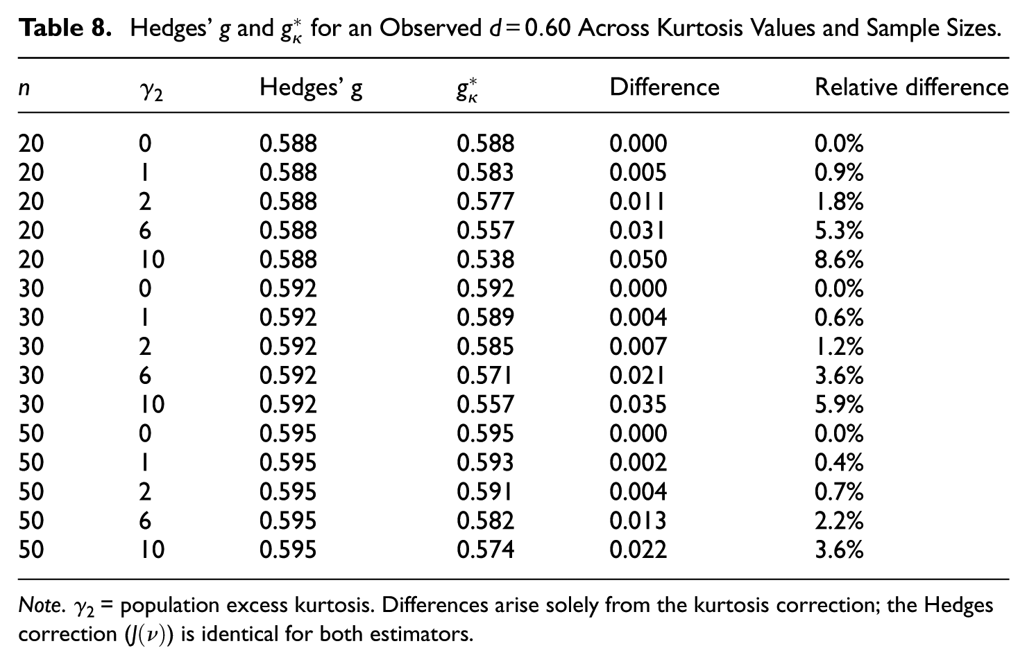
Table 8 presents the practical impact of $g_{κ}^{*}$ for a range of kurtosis values typical of real data, at the sample sizes common in behavioral and educational research. We assume a hypothetical study yielding an observed Cohen’s $d = 0.60$ (a medium-to-large effect) with equal group sizes.

Three patterns are noteworthy. First, when $γ_{2} = 0$ (normality), g and $g_{κ}^{*}$ are identical, confirming backward compatibility. Second, the adjustment is practically negligible ( $< 1 %$ ) for $γ_{2} \leq 1$ (e.g., 0.4%–0.9% across the sample sizes in Table 8), which covers the majority of normally behaved educational test score data, and remains modest (about 0.7%–1.8%) at $γ_{2} = 2$ . Third, for moderately-to-highly leptokurtic data ( $γ_{2} = 6$ –10, common in reaction time and clinical data), the adjustment is 2% to 9% of the effect size, depending on sample size. At $n = 20$ with $γ_{2} = 10$ , the difference of 0.050 represents a meaningful shift: in a meta-analysis, this systematic overestimation would accumulate across studies.

Meta-Analytic Implications

Consider a fixed-effect meta-analysis of $k = 30$ reaction time studies (where k denotes the number of independent primary studies being pooled), each with $n = 25$ per group and a true effect of $δ = 0.50$ . Reaction time data typically exhibits $γ_{2} \approx 6$ (DeCarlo, 1997). For each study, the residual bias of Hedges’ g is approximately $3 δ γ_{2} / (8 \tilde{n}) = 3 (0.50) (6) / (8 \times 50) \approx 0.023$ . This per-study bias is common to all studies and does not cancel in the weighted average; the pooled fixed-effect estimate inherits the same systematic bias of 0.023. Meanwhile, the standard error of the pooled estimate shrinks to approximately ${SE}_{per - study} / \sqrt{k} \approx 0.287 / \sqrt{30} \approx 0.052$ . The ratio of systematic bias to pooled standard error is therefore $0.023 / 0.052 \approx 0.43$ , which is nontrivial. Using $g_{κ}^{*}$ instead of Hedges’ g in each primary study would remove this bias at the source, requiring only that researchers report ${\hat{γ}}_{2}$ alongside the effect size—an easy addition to the standard reporting template.

Discussion

Summary of Findings

This article proposed $g_{κ}^{*}$ , a kurtosis-adjusted bias correction for the SMD that uses the exact Hedges correction as its anchor. The key findings from the Monte Carlo simulation (315 main conditions plus 90 Tukey’s g-and-h conditions, each condition replicated 10,000 times; the $10^{6}$ draws mentioned in Section “Results: g-and-h Distributions” were used only once, to estimate the population standardization constants for the g-and-h family, not as a replication count) are as follows:

Under heavy-tailed distributions ( $γ_{2} \geq 4$ ), $g_{κ}^{*}$ reduced the residual bias of Hedges’ g by 36%–92% at sample sizes of 20–100 per group, with the largest reductions occurring at larger sample sizes and higher kurtosis values.

The 95% CI achieved coverage of .952–.961 under heavy-tailed distributions, compared with .938–.947 for Hedges’ g, .954–.961 for Bonett (2008), and .926–.956 for BCa bootstrap in the 24 selected conditions examined (Section “Results: Comparison With BCa Bootstrap”). The $g_{κ}^{*}$ interval achieved comparable coverage to Bonett with consistently narrower intervals.

Under normality, $g_{κ}^{*}$ algebraically reduces to Hedges’ g when ${\hat{γ}}_{2} = 0$ . In finite samples from normal populations, ${\hat{γ}}_{2}$ fluctuates around zero, producing negligible differences between $g_{κ}^{*}$ and g (within Monte Carlo error in all conditions examined).

The g-and-h analysis (Section “Results: g-and-h Distributions”) confirmed that the correction effectively captures kurtosis regardless of its source (pure kurtosis or skewness-induced kurtosis), but has diminished effectiveness when extreme kurtosis and severe skewness co-occur.

The estimator maintained its advantages under unequal sample sizes and under moderate variance heterogeneity ( $σ_{2} / σ_{1} = \sqrt{2}$ ), though coverage degraded under more extreme heterogeneity combined with heavy tails.

Comparison With Bonett

The Bonett (2008) approach and the proposed $g_{κ}^{*}$ differ in what they modify: Bonett adjusts only the variance estimator, leaving the point estimate as Hedges’ g, while $g_{κ}^{*}$ adjusts both the point estimate and the variance estimator. The simulation shows that both achieve similar coverage improvement, but $g_{κ}^{*}$ achieves this with (a) a less-biased point estimate and (b) slightly narrower intervals. For example, under the exponential distribution at $n = 50$ and $δ = 0.5$ , the Bonett interval has width 0.860 and coverage .961, while $g_{κ}^{*}$ achieves coverage .959 with width 0.846—a 1.6% narrower interval at comparable coverage. The narrower intervals arise because correcting the bias in the point estimate reduces the systematic error that must otherwise be accommodated by interval width.

Practical Recommendations

When to Use

The benefit of $g_{κ}^{*}$ is greatest when data are leptokurtic ( ${\hat{γ}}_{2} > 2$ ) and the sample size is moderate ( $15 \leq n \leq 50$ ). At very large sample sizes ( $n > 200$ ), the bias of Hedges’ g is already negligible. Computationally, $g_{κ}^{*}$ is a closed-form statistic requiring no iteration or resampling: its cost is a single $O (N)$ pass over the data to obtain the pooled second and fourth moments, in contrast to the $B \times R$ resamples required by bootstrap intervals. In our benchmark (reported in the Online Supplement, Supplementary Section S2), evaluation completed in well under a millisecond per sample for $n \leq 1, 000$ per group. The estimator reverts exactly to Hedges’ g when ${\hat{γ}}_{2} = 0$ .

Reporting

We recommend reporting ${\hat{γ}}_{2}$ alongside $g_{κ}^{*}$ . This enables readers to assess the magnitude of the kurtosis adjustment and facilitates future meta-analytic use. When $| {\hat{γ}}_{2} | < 1$ , the adjustment is minimal and $g_{κ}^{*} \approx g$ . Because $g_{κ}^{*}$ assumes a common population variance (Assumption A2), we further recommend reporting the two group variances (or standard deviations) separately, so that readers can gauge the plausibility of the homoscedasticity assumption and, where it is questionable, consider a heteroscedastic estimand instead.

Scope

The estimator requires individual participant data (or at least group-level fourth moments). It is therefore positioned primarily as a tool for primary research. In meta-analysis, it can be used when IPD is available or when primary studies report kurtosis, but it cannot be applied retrospectively to studies reporting only means and SDs.

Limitations

Several limitations warrant discussion. First, the proposed correction assumes equal population variances (Assumption A2). The robustness analysis (Table 7) showed that under moderate heterogeneity ( $σ_{2} / σ_{1} = \sqrt{2}$ ), $g_{κ}^{*}$ continues to reduce bias relative to Hedges’ g for the heavy-tailed distributions (where the kurtosis correction is operative), while for the normal distribution the two estimators differ only within Monte Carlo error. Coverage degrades notably under severe heterogeneity ( $σ_{2} / σ_{1} = 2$ ) combined with heavy tails (e.g., coverage of .928 for the exponential distribution). Extension to heteroscedastic settings, where the estimand itself becomes ambiguous between Glass’Δ and Cohen’s d, is a priority for future work.

Second, the plug-in estimate ${\hat{γ}}_{2}$ is noisy at small sample sizes ( $n < 15$ ); Section “Plug-in Estimation Error” provides a theoretical analysis showing the plug-in error is $O (n^{- 2})$ , but practical variance in ${\hat{γ}}_{2}$ can still induce instability. The shrinkage variant discussed in Remark 3 merits systematic investigation.

Third, the second-order Taylor expansion captures the dominant nonnormality effect through the kurtosis term but does not explicitly correct for skewness. The covariance analysis in Section “Independence of Numerator and Denominator” shows that skewness contributes $O (γ_{1} n^{- 3 / 2})$ to the bias, which is of lower order than the kurtosis term $O (γ_{2} n^{- 1})$ . A joint skewness–kurtosis correction may offer further improvements for strongly asymmetric distributions and is a direction for future work.

Fourth, the g-and-h analysis (Section “Results: g-and-h Distributions”) revealed that when both severe skewness ( $γ_{1} > 2$ ) and extreme kurtosis ( $γ_{2} > 10$ ) are present simultaneously, $g_{κ}^{*}$ reduces only 15% to 24% of the bias and coverage remains below .950 for larger n. This indicates that a joint skewness–kurtosis correction—addressing the numerator–denominator covariance structure analyzed in Section “Independence of Numerator and Denominator”—would be needed for such extreme distributions. This is a direction for future work.

Fifth, the BCa bootstrap comparison (Section “Results: Comparison With BCa Bootstrap”) showed that BCa coverage fell below the nominal level under nonnormal distributions at $δ = 0.8$ (coverage .926–.953), whereas $g_{κ}^{*}$ maintained .942–.955. In the present simulation conditions, BCa did not fully correct the coverage loss, suggesting that nonparametric resampling may not reliably capture the finite-sample bias structure of the SMD under heavy-tailed nonnormality. The computational cost of BCa ( $B \times R$ resamples per study) further limits its practical utility compared with the closed-form $g_{κ}^{*}$ .

Sixth, regarding robust effect sizes based on trimmed means (Algina et al., 2005; Keselman et al., 2008): these methods estimate a fundamentally different estimand—the standardized difference in trimmed means—and are therefore not directly comparable with $g_{κ}^{*}$ in terms of bias or MSE. The advantage of $g_{κ}^{*}$ is that it preserves the conventional estimand $δ = (μ_{1} - μ_{2}) / σ$ , ensuring backward compatibility with the existing literature and meta-analytic infrastructure. When robustness to outliers is paramount and a change of estimand is acceptable, trimmed-mean effect sizes remain a valuable alternative.

Seventh, the proposed estimator improves the statistical properties of the conventional SMD estimator but does not address the interpretability of δ under nonnormality. As Hedges (2025) demonstrated, overlap-based interpretations of the SMD (e.g., Cohen’s $U_{3}$ ) can be misleading when distributional assumptions are violated. When the research goal requires meaningful interpretation of distributional overlap rather than a location-shift summary, researchers should consider whether the conventional SMD is the appropriate target estimand.

Eighth, the confidence interval (equation (14)) relies on a normal-approximation assumption that we have not formally proven for $g_{κ}^{*}$ under nonnormality. While such a result is plausible from the joint asymptotic normality of $(d, {\hat{γ}}_{2})$ under standard moment conditions, a formal proof is beyond the present scope. The Monte Carlo results in Sections “Results: Coverage–Width Trade-off” and “Results: Comparison With BCa Bootstrap” provide empirical evidence that the normal-approximation interval performs well in moderate samples ( $n \geq 20$ ) under the distributions examined, but they should be regarded as heuristic confirmation rather than a theoretical guarantee. A rigorous derivation of the asymptotic distribution of $g_{κ}^{*}$ , together with an examination of the empirical sampling distribution at larger sample sizes, is a natural direction for future work.

Conclusion

The kurtosis-adjusted estimator $g_{κ}^{*}$ provides a principled, closed-form correction that bridges a gap between statistical theory and empirical practice. By using the exact Hedges correction as its anchor and incorporating a simple multiplicative kurtosis adjustment, it offers improved bias and coverage without changing the target estimand or sacrificing computational simplicity. We recommend its use as a low-cost default correction in primary research where data are expected to be leptokurtic ( ${\hat{γ}}_{2} > 2$ ) and sample sizes are moderate ( $15 \leq n \leq 50$ ), provided that variance heterogeneity is not extreme. In such settings, the absolute bias reduction is typically .005 to .02 in effect size units—small in any single study, but systematic and cumulative across a literature. When data are approximately normal or sample sizes are large, $g_{κ}^{*}$ behaves essentially identically to Hedges’ g and imposes no unnecessary adjustment. The correction is not a substitute for careful distributional diagnostics or for robust estimands when nonnormality is extreme (Hedges, 2025); rather, it offers a targeted improvement for the conventional SMD in the realistic regime where mild-to-moderate nonnormality is present but a change of estimand is unwarranted.

Supplemental Material

sj-docx-1-epm-10.1177_00131644261461535 – Supplemental material for A Kurtosis-Adjusted Bias Correction for the Standardized Mean Difference: Extending Hedges’ g to Nonnormal Populations

Supplemental material, sj-docx-1-epm-10.1177_00131644261461535 for A Kurtosis-Adjusted Bias Correction for the Standardized Mean Difference: Extending Hedges’ g to Nonnormal Populations by Daiki Nakamura in Educational and Psychological Measurement

Footnotes

ORCID iD

Daiki Nakamura

Ethical Considerations

This study does not involve human participants, human data, or human tissue. All analyses were conducted on simulated data generated by Monte Carlo methods and on publicly available data sets. Ethical approval was not required.

Consent to Participate

Not applicable.

Consent for Publication

Not applicable.

Funding

The author received no financial support for the research, authorship, and/or publication of this article.

Declaration of Conflicting Interests

The author declared no potential conflicts of interest with respect to the research, authorship, and/or publication of this article.

Data Availability Statement

All simulation code (R 4.5.3), raw simulation results (CSV), and supplementary tables are publicly available at .

Supplemental Material

Supplemental material for this article is available online.

References

Algina

Keselman

H. J.

Penfield

R. D.

(2005). An alternative to Cohen’s standardized mean difference effect size: A robust parameter and confidence interval in the two independent groups case. Psychological Methods, 10(3), 317–328. https://doi.org/10.1037/1082-989X.10.3.317

Algina

Keselman

H. J.

Penfield

R. D.

(2006). Confidence interval coverage for Cohen’s effect size statistic. Educational and Psychological Measurement, 66(6), 945–960. https://doi.org/10.1177/0013164406288161

American Psychological Association. (2020). Publication manual of the American Psychological Association (7th ed.)

Blanca

M. J.

Arnau

López-Montiel

Bono

Bendayan

(2013). Skewness and kurtosis in real data samples. Methodology, 9(2), 78–84. https://doi.org/10.1027/1614-2241/a000057

Bonett

D. G.

(2008). Confidence intervals for standardized linear contrasts of means. Psychological Methods, 13(2), 99–109. https://doi.org/10.1037/1082-989X.13.2.99

Borenstein

Hedges

L. V.

Higgins

J. P. T.

Rothstein

H. R.

(2009). Introduction to meta-analysis. John Wiley & Sons.

Cohen

(1988). Statistical power analysis for the behavioral sciences (2nd ed.). Lawrence Erlbaum Associates.

Cumming

(2014). The new statistics: Why and how. Psychological Science, 25(1), 7–29. https://doi.org/10.1177/0956797613504966

DeCarlo

L. T.

(1997). On the meaning and use of kurtosis. Psychological Methods, 2(3), 292–307. https://doi.org/10.1037/1082-989X.2.3.292

10.

Efron

Tibshirani

R. J.

(1993). An introduction to the bootstrap. Chapman & Hall/CRC.

11.

Hedges

L. V.

(1981). Distribution theory for Glass’s estimator of effect size and related estimators. Journal of Educational Statistics, 6(2), 107–128. https://doi.org/10.3102/10769986006002107

12.

Hedges

L. V.

(2025). Interpretation of the standardized mean difference effect size when distributions are not normal or homoscedastic. Educational and Psychological Measurement, 85(2), 245–257. https://doi.org/10.1177/00131644241278928

13.

Hedges

L. V.

Olkin

(1985). Statistical methods for meta-analysis. Academic Press.

14.

Hoaglin

D. C.

(1985). Summarizing shape numerically: The g-and-h distributions. In Hoaglin

D. C.

Mosteller

Tukey

J. W.

(Eds.), Exploring data tables, trends, and shapes (pp. 461–513). John Wiley & Sons.

15.

Joanes

D. N.

Gill

C. A.

(1998). Comparing measures of sample skewness and kurtosis. Journal of the Royal Statistical Society: Series D (The Statistician), 47(1), 183–189. https://doi.org/10.1111/1467-9884.00122

16.

Kelley

(2005). The effects of nonnormal distributions on confidence intervals around the standardized mean difference: Bootstrap and parametric confidence intervals. Educational and Psychological Measurement, 65(1), 51–69. https://doi.org/10.1177/0013164404264850

17.

Keselman

H. J.

Algina

Lix

L. M.

Wilcox

R. R.

Deering

K. N.

(2008). A generally robust approach for testing hypotheses and setting confidence intervals for effect sizes. Psychological Methods, 13(2), 110–129. https://doi.org/10.1037/1082-989X.13.2.110

18.

Lakens

(2014). Stroop task dataset [Data set]. GitHub. https://github.com/Lakens/Stroop

19.

Micceri

(1989). The unicorn, the normal curve, and other improbable creatures. Psychological Bulletin, 105(1), 156–166. https://doi.org/10.1037/0033-2909.105.1.156

20.

Stuart

Ord

J. K.

(1994). Kendall’s advanced theory of statistics (6th ed., Vol. 1). Edward Arnold.

Supplementary Material

Please find the following supplemental material available below.

For Open Access articles published under a Creative Commons License, all supplemental material carries the same license as the article it is associated with.

For non-Open Access articles published, all supplemental material carries a non-exclusive license, and permission requests for re-use of supplemental material or any part of supplemental material shall be sent directly to the copyright owner as specified in the copyright notice associated with the article.

0.57 MB

n	$t (5)$	Lognormal	Exp	$χ^{2} (3)$
10	13%	14%	19%	22%
15	20%	32%	32%	36%
20	43%	36%	62%	40%
30	45%	57%	50%	59%
50	57%	68%	61%	49%
100	53%	75%	92%	60%

n	$t (5)$	Lognormal	Exp	$χ^{2} (3)$
10	13%	14%	19%	22%
15	20%	32%	32%	36%
20	43%	36%	62%	40%
30	45%	57%	50%	59%
50	57%	68%	61%	49%
100	53%	75%	92%	60%

n	$t (5)$	Lognormal	Exp	$χ^{2} (3)$
10	13%	14%	19%	22%
15	20%	32%	32%	36%
20	43%	36%	62%	40%
30	45%	57%	50%	59%
50	57%	68%	61%	49%
100	53%	75%	92%	60%