Revisiting the Gravity Model of Migration

Abstract

The recent global migration pattern indicates the importance of the movement of people from developing countries to developed countries in search of better economic opportunities. The G20 report of ‘International Migration and Displacement Trends’ mentions India at the top of the list of highly educated emigrants in G20 countries. The current study addresses the endogeneity problem in the migration determinants and attempts to highlight the major regional and economic determinants of migration flow from India to major OECD countries using the Gravity model of migration. We apply the Prais–Winsten regression method to address the cross-sectional correlation, while we apply instrumental variable regression and Hausman–Taylor regression estimation techniques to deal with the endogeneity issue. The findings reveal that the population of India, distance, common official language and per capita income differential are the major determinants of migration from India. In the backdrop of our findings, in terms of per capita income differential, there is a need for an upward revision in the pay scale of the white-collar workers in the organised sector.

JEL Codes: C23, F22, J11, J60

Keywords

International migration population unemployment panel data endogeneity

Introduction

Theoretically, the gravity model of migration is usually based on the Random Utility Maximisation (RUM hereafter) model. The RUM model describes the utility an individual gets by living in a particular country compared to the expected utility of moving to an alternative place. The RUM model assumes that the pull factors (like better employment opportunities) in the migrants’ destination should not be affected by the migration flow itself. Ramos (2016), however, believes that the attractiveness of a region due to its low levels of unemployment compared to migrants’ origin region stimulates the inflows of immigrants. Consequently, unemployment in this region may increase while it may parallelly decline in the origin region. Gravity models do not incorporate these second-round repercussions; hence, they may give misleading conclusions. Such explanatory factors that are not affected by the current period migration flows but may be affected by the immediate past periods’ migration flows are called predetermined variables in time series or panel data settings. These panel data gravity models can be empirically applied even in the presence of predetermined variables, provided that the migration flow (i.e., the dependent variable) is not serially correlated. However, several studies related to migration suggest that past periods’ migration movements affect the current flows (e.g., Disney et al., 2015; Epstein & Gang, 2006; Greenwood, 1970; Zimmer, 2008, among others). Such migration movements might cause the problem of endogeneity in the above-discussed predetermined variables.

Nonetheless, in an empirical framework, gravity model can be successfully used after taking due care of the possible endogeneity problem owing to these second-round effects. Most of the previous works concerning the migration flow, especially from developing countries to developed countries, do not address the issue of endogeneity. For example, the population of both the destination and source countries and the existing diaspora of the migrants’ source country may be endogenous. The endogeneity occurs either due to the bidirectional causality (for instance, the populations in both the regions may also be affected by the volume of migration in that period) or because of omission of some important variables from the model, which might affect other explanatory variables included in the model. For instance, the educational status of the migrants, if not included in the model, might affect the prevailing employment rates difference between the countries. Such a problem induces biases in the estimates of the model and makes the drawn conclusion less reliable.

Another critical issue in the panel data models is the cross-sectional (or contemporaneous) correlation among the errors of different groups due to the presence of common shocks or spatial dependence or unobserved factors that are ultimately subsumed in the errors. If the cross-sectional correlation is due to the common factors, then applying the traditional fixed effect and random effect models gives consistent estimates, though the standard errors are biased. The empirical estimation in the present study addresses the problems mentioned above using the Prais–Winsten regression (Prais & Winsten, 1954) with panel-corrected standard error (PCSE), instrumental variable regression (IVREG) and Hausman–Taylor regression (HTREG; Hausman & Taylor, 1981). Contrary to some previous research works based on gravity models of migration, our findings through these techniques reveal new explanations to some of the migration determinants and hence fetch novelty to this work. We find a plethora of empirical studies examining the determinants of migration from various aspects. However, the present findings give a better picture of unilateral migration flows, which are more prevalent these days.

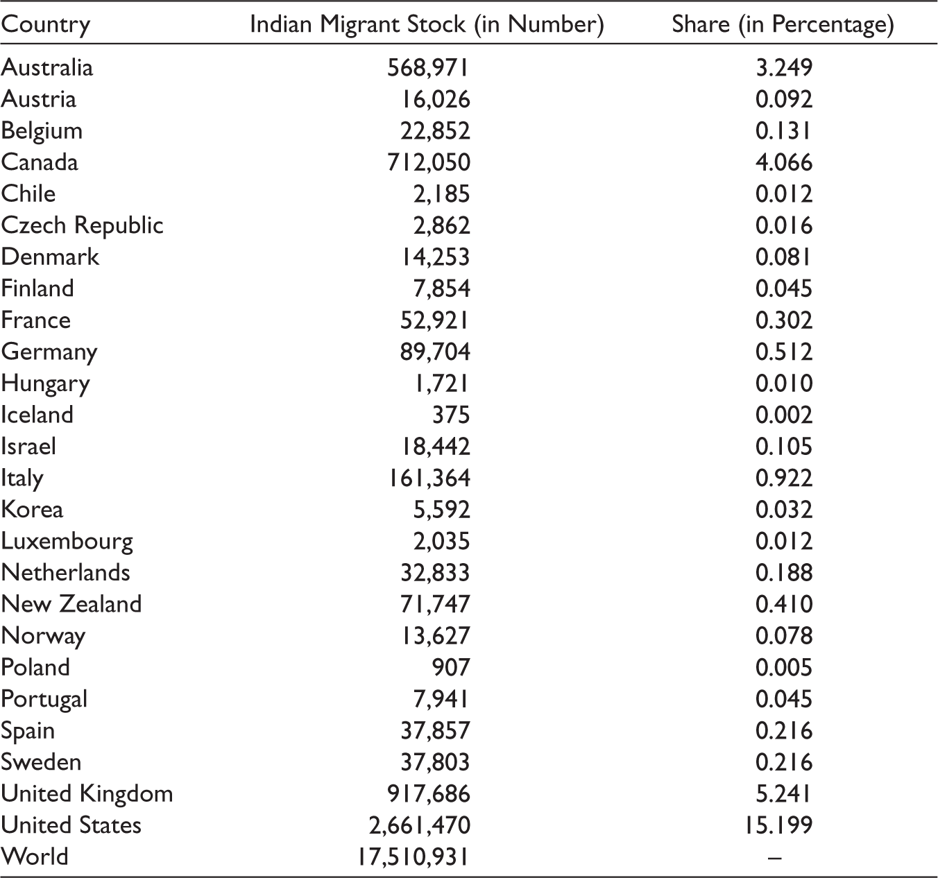
Moreover, taking India as a migration source to the OECD countries in our sample adds to our knowledge of migration’s determinants as we do not find any such study on Indian emigration to the developed counties. Since India has emerged as one of the few leading emigration source countries and is expected to be at the top in this regard soon, understanding India’s migration anatomy is of great value to demographers, migration policymakers and economists globally. Examining the role of major demographic, economic, political and geographic determinants of migration from India in the present work unfolds new facts, as all the determinants do not necessarily depict the same behaviour as shown in earlier studies. Therefore, the current study highlights some of the aforementioned determinants of migration flow from the developing country (India, here) to the developed nations taking the analogy from Newton’s law of gravity. Here, we examine the flow of Indian migrants to 25 selected OECD countries for the period from 2001 to 2019.¹ Table 1 depicts the stock of Indian migrants in each sample country and their share in total Indian migrants in 2019. Total Indian migrants’ stock in the world was approximately 17.5 million in 2019. The United States homes the largest number of Indian migrants among all the OECD countries, with about 15% of total Indian migrants globally. Besides the United States, the United Kingdom, Canada and Australia are the other major destinations for Indian migrants, with 5.2%, 4.06% and 3.24% of total Indian migrants globally, respectively. In total, all the OECD countries chosen in the current sample constitute 31.18% of the world total in terms of homing Indian migrants.

Table 1.

Stock of Indian Migrants in Sample OECD Countries in 2019.

Country	Indian Migrant Stock (in Number)	Share (in Percentage)
Australia	568,971	3.249
Austria	16,026	0.092
Belgium	22,852	0.131
Canada	712,050	4.066
Chile	2,185	0.012
Czech Republic	2,862	0.016
Denmark	14,253	0.081
Finland	7,854	0.045
France	52,921	0.302
Germany	89,704	0.512
Hungary	1,721	0.010
Iceland	375	0.002
Israel	18,442	0.105
Italy	161,364	0.922
Korea	5,592	0.032
Luxembourg	2,035	0.012
Netherlands	32,833	0.188
New Zealand	71,747	0.410
Norway	13,627	0.078
Poland	907	0.005
Portugal	7,941	0.045
Spain	37,857	0.216
Sweden	37,803	0.216
United Kingdom	917,686	5.241
United States	2,661,470	15.199
World	17,510,931	–

Source: Department of Economic and Social Affairs and authors’ calculation.

Note: All the figures mentioned here are taken from the Department of Economic and Social Affairs, United Nations as of 2019.

It is assumed that migration happens due to low human capital in the source countries and more employment opportunities in OECD countries. Therefore, the present study tries to identify such economic determinants of migration from India to OECD countries. The specific countries considered for the present study have high human capital and set the standard of living in terms of economic and social aspects. It may give policymakers an idea to pay attention to the cause and effects of migratory movements from India to OECD countries. We use the population of India, the population of selected OECD countries and the distance of each country from India as the major determinants of migration to OECD countries. Among other important economic factors used in the study are the differences in the per capita income between destination country and India, proximity in official languages in both India and destination countries, the difference in the level of unemployment and some other controls. The study finds that the population of India, per capita income differential, distance and common official language are the major determinants of migratory flows from India to OECD countries. Additionally, the population in the destination country and difference in the degree of control of corruption have weak impacts on migration volume. These findings have important policy implications, which are discussed in the last section.

Historical Background and Motivation

Although Tinbergen (1962) is known for pioneering the application of the gravity model in international trade, the history of the gravity model of migration is even older and dates back to Ravenstein (1885), who uses the gravity model for the study of the movement of people from country to country. However, the gravity model of migration did not get prominence until recently after the availability of dyadic nature migration data. The spatial interactions among the nations through trade and migration are easily and more accurately estimated after incorporating the theoretical foundation of the gravity model of Anderson (2011). In the gravity model of international trade, the trade is driven by the GDP of both the trading countries. Similarly, the migration flow is driven by the forces between migrants’ native countries and destination countries and impeded by the cost of moving from one country to another. First, the global migration pattern indicates the importance of the movement of people from developing countries to developed countries. The share of international migrants living in the OECD countries has continuously been increasing since 2000, and it was as high as 54% of the total in 2015–2016 (OECD, 2019b). As per the G20 ‘International Migration and Displacement Trends’ report (OECD, 2019a), one-fifth of the entire foreign-born population aged 15 or over in G20 countries emigrate from five countries, with Mexico topping the list (11.7 million emigrants), and India at the second position (6.8 million emigrants). The remaining are Bangladesh (4.9 million emigrants), Ukraine (4.8 million emigrants) and China (4.7 million emigrants). The same report also mentions the countries with the largest immigrant population from 2010 to 2018; the United States remains at the top, followed by Saudi Arabia, Germany, Australia and Canada.

Early traditional migration studies primarily consider the disequilibrium approach.² This view of migration can be traced back to the writings of J. R. Hicks in his book The Theory of Wages (Hicks, 1932). Based on the analyses of early researchers, he concludes that the differences in wages and other economic opportunities are the primary motivating factors for migration. Migration works since the early 1980s started emphasising the equilibrium approach, which assumes that spatial wage differentials reflect (entirely or significantly) compensating differentials that are related with the spatial differences in the amenities in the two regions and do not reflect opportunities for utility gains as highlighted by Graves (1980). Migration in today’s world is primarily driven by economic factors, barring the movement of refugees or illegal migrants. A significant population from the developing countries move to the developed countries in search of better employment opportunities. Generally, the migration flows are bidirectional wherein the populations of two countries move into each other, but the unidirectional migration flow is also an interesting phenomenon as it unfolds the major economic causes of migration happening in the world.

There has been a considerable unidirectional movement of citizens from developing countries to developed countries during the last two decades. Such unidirectional flow of migrants is called the emigration in the source country, while it is called immigration in the destination country. There was a considerable migration of Indian rural and unskilled workers, particularly to the Middle East and Southeast Asia. In contrast, most of the skilled and educated workers migrated to developed countries such as the United States, Germany, the United Kingdom, Canada and Australia among others. It implies that Indian migration to OECD countries primarily consists of skilled workers. The G20 report of ‘International Migration and Displacement Trends’ mentions that the largest number of educated immigrants in G20 countries are from India (51%), followed by the Philippines (48.9%), the United Kingdom (48.4%) and China (47.7%). India is also the largest remittances receiving country, followed by China, Philippines, Mexico and Pakistan. Naujoks (2009) states that the migration of the Indian population to countries across the globe will continue to interest researchers and policymakers in future periods because of its most diverse and complex migration history in the world.

The article proceeds as follows. In the second section, we do a literature survey of the theoretical as well as empirical studies concerning migration. The third section discusses the empirical model, data description and methodology. In the fourth section, we present the preliminary analysis. The fifth section is devoted to the results and discussion. The final section concludes the article.

Literature Review

In the last two decades, there has been growing interest in explaining the gross international migration flows with the help of gravity models (Mayda, 2010; Ramos, 2016). We divide this section into two parts based on two broad categories, namely demographic, geographic and social (population, existing diaspora, age structure, infant mortality rate, urbanisation, distance, climate, language, culture, political stability, government effectiveness and the rule of law) and economic (income difference, unemployment rate, trade volume, foreign investment, degree of openness, information and technology and human capital) determinants of migration.

Demographic, Geographic and Social Determinants

Lewer and Van den Berg (2008) have worked on OECD countries’ migration by fitting a gravity model on immigrants. They find a positive and significant effect of the population in both source and destination countries on the immigration in the destination countries. Diaspora of the migration origin country has also been used as one of the essential determinants of migration. Utilising the information on bilateral international migration by educational attainment from 195 countries to 30 developed countries from 1990 to 2000, Beine et al. (2009) find that the diasporas encourage migration flows, inversely affect the average educational level and increase the concentration of low-skill migrants. Interestingly, diasporas explain most of the variability of migration flows and selection. Kim and Cohen (2010) show that populations of both source and destination countries, infant mortality rate in the destination and the distance between the destination and source countries turn out to be the major determinants of migration outflows. In contrast, primary determinants of the migration inflows are the infant mortality rate in the source country and land area of the destination country, besides the four factors mentioned above. The population of both regions have positive impacts, and distance negatively impacts both kinds of migration flows.

Moreover, a younger age structure in one of the sample countries discourages the migration inflows and promotes the migration outflows. The potential support ratio (PSR), an indicator of the young age structure (total people aged 15–64 per person aged 65 or over), mildly promotes the inflows and substantially promotes outflows. In contrast, in the destination country, a higher PSR considerably discourages inflows and slightly discourages outflows. Urbanisation in both source and destination countries, common official languages and colonial links significantly increase inflows. Lastly, inflows are negatively affected if the destination and origin are landlocked.

Examining the role of climatic factors, Beine and Parson (2015) show no strong evidence of the direct effect of these factors on long-run international migration. However, these climatic factors indirectly affect migration flows; for instance, natural disasters and shortage of rainfall in the migration source country compared to destinations country, widen the wage-gap between them and, thereby promote international migratory flows. Adsera and Pytlikova (2015) use the data on immigration to 30 OECD destination countries from the rest of the world for the period 1980–2010 and highlight that linguistic proximity and English, as the official language of destination, increase the migration flows. Alimi et al. (2019) highlight the role of demographic factors. Their finding suggests that youthfulness encourages outward migration, while agedness impedes it from urban areas. Examining the role of climatic factors, they find that people in sunnier areas have low outmigration tendencies. The effect of rainfall is mixed on different kinds of migratory flows.

Economic Determinants

By using a standard labour market study, Friedberg and Hunt (1995), Card (2001) and Borjas (2003) propose that an immigrant worker responds to differences in earnings between countries. Similarly, utilising the information on migration from 74 origin countries to 14 OECD countries for the period 1980–2005, Ortega and Peri (2009) show that the flow of migrants is enhanced by a positive wage differential between origin and destination, while it is dampened by the more restrictive immigration policies in the later. Skilled migration constitutes a substantial portion of total global migration and has resulted in a much-debated issue called ‘brain drain’ or ‘human capital flight’ in developing countries. Docquier et al. (2007) examine the determinants of brain drain and highlight the cross-country differences in the migration of skilled labour for the period ranging from 1990 to 2000. Countries adjacent to major OECD regions—with colonial links with OECD countries, with most people moving to countries with quality-selective immigration programmes—have strong degrees of brain drain. Furthermore, the brain drain is positively related to political instability and the degree of fractionalisation in the origin countries and is negatively affected by natives’ human capital.

Using average trade tariffs and bilateral exchange rate volatility as instruments for trade flows, Campaniello (2014) analyses the impact of trade on migration from the Southern Mediterranean to the European Union for the period 1970–2000. He finds that migration and trade from the Southern region to the European Union are positively and significantly correlated. Jandová and Paleta (2015) for the Czech region find that the economic variables—such as average wage, registered unemployment rate and job vacancies for internal migration—give slightly improved results than the pure gravity model. They further highlight that the economic variables in the ratio form have better explanatory power than their representation in differences and values. This implies that migrants are more interested in ‘how many times’ rather than ‘how much’. Alimi et al. (2019) find noteworthy differences in the impact of migration determinants when comparing urban–urban, urban–rural and urban–world migration flows. Considering the economic determinants, they find that the interurban migration flow is positively affected by the income growth in the destination region and inversely affected by income growth in the source region. Income growth also promotes the flows of international migrants to New Zealand but does not significantly affect the rural–urban migration flows within New Zealand. Furthermore, they find that increasing inequality leads to higher migration outflows and higher migration inflows into urban areas. However, there is no evidence of such effect of inequality growth for migration to and from the rural areas. In the case of international migration, the positive impact of inequality growth on immigration in the destination region is weak. The level of human capital (measured by the proportion of the population having at least a bachelor’s degree) positively impacts the migration flows to and from urban areas with a greater proportion of the population with tertiary education. The pull effect of human capital is found stronger than the push effect.

Parallelly, there are other works concerning the bidirectional causality between migration and economic variables. Utilising the information on 22 OECD countries for the period from 1987 to 2009, Boubtane et al. (2013) examine the bidirectional causality between immigration and host country economic conditions and find evidence of migration promoting economic prosperity and vice versa. Migration positively affects GDP per capita and negatively affects total unemployment. At the same time, migration gets promoted by an increasing GDP per capita of the host country and is inhibited by the total unemployment rate in the host country.

Presently, studies on migration address various new dimensions such as the dynamic pattern of migration, spatial analysis and the role of information and technology. On the same line, Fan et al. (2018) examine the spatio-temporal characteristics of interprovincial migration in China. They find that geographical proximity positively impacts interprovincial population migration; interprovincial immigration and emigration both have increased with economic development; adoption of the historical dependent variable and the spatial lag factor greatly adds to the explanatory power in modelling the interprovincial migration in China. The recent increasing use of the Internet for job availability also gives good information about the potential international migrants. Mamertino and Sinclair (2019), using the data on the online job seekers outside their home country, highlight that online job search is positively correlated with the realised migration. Applying the gravity model, they also provide evidence of the online job search variable responding similarly to the determinants of migration as the migration itself.

Pu et al. (2019) employ the space-time dimension in the gravity equation to model dyadic interprovincial migration flows in China from 1985 to 2015. They decompose the origin, destination and spillover effects into their contemporaneous short-term and long-term components. The findings suggest that space–time interactions play a crucial role in migration flows. Population size and age structure are the essential determinants of China’s interprovincial migration. Moreover, economic development tends to have an inverted U-shaped relationship with migration, which is not highlighted in nonspatial models. In the present world, skilled migration has gained more momentum as well as the attention of the researcher and policymakers as it constitutes a substantial portion of total global migration. Biavaschi et al. (2020) show that global migration is profoundly skill-biased, with tertiary-educated workers having a migrating tendency four times larger than workers with lower education. Another important and relatively new aspect of migration studies is the multilateral resistance to migration, similar to the idea of multilateral trade resistance given by Anderson and Van Wincoop (2004). This idea implies that dyadic migration does not entirely depend on the attractiveness of the migration destination but also on the scope of moving to other destinations. Bertoli and Moraga (2013) apply the common correlated effect estimator of Pesaran (2006) to high-frequency Spanish administrative data on bilateral migration flows between 1997 and 2009. They find that economic determinants significantly affect bilateral migration flows and immigration policies.

Empirical Model, Data and Methodology

Historically, research works have shown that the migration source countries are mostly underdeveloped or developing, while the migration destination countries are mainly the developed ones. The volume of migration flow is primarily determined by the population size of both the source and destination countries. Under ceteris paribus, the more people there are in a source country and the more people are likely to migrate as a large population is always a challenge for the governments, especially in the developing countries, to provide for education, health and other basic amenities of life. Similarly, the larger the population in the destination country, higher are the labour market opportunities for immigrants. The reason is that a developed country with a high population also has a larger economic size. Such a country has a sufficiently sizeable skilled population, but there is a dearth of manual labour to maintain a balance.

Similarly, we can assume the migration to be negatively related to the distance between the two countries because the costs associated with the migration generally increase with the distance. Furthermore, cultural differences are also expected to be large between the two countries if they are far apart. These differences also act as a hindrance in the movement of people more attached to their culture and language. On the contrary, if two countries are close or share the border or are in the same continent, they are expected to have similarities in their cultures and sometimes, in languages. These cultural similarities motivate the migrants to move from their origin country to the neighbouring country compared to a distant one with the same economic opportunities. Considering the role of the factors mentioned above, we can fit our empirical model of Indian migration to selected OECD countries by taking the analogy from Newton’s law of gravity.

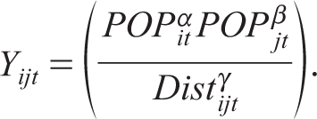
In its simplest form, gravity equation of immigration (or migration) can be written as follows:

Y_{i j t} = (\frac{P O P_{i t}^{α} P O P_{j t}^{β}}{D i s t_{i j t}^{γ}}) .

Y_{i j t} = (\frac{P O P_{i t}^{α} P O P_{j t}^{β}}{D i s t_{i j t}^{γ}}) .

Y_{i j t} = (\frac{P O P_{i t}^{α} P O P_{j t}^{β}}{D i s t_{i j t}^{γ}}) .

Y_{i j t} = (\frac{P O P_{i t}^{α} P O P_{j t}^{β}}{D i s t_{i j t}^{γ}}) .

(1)

By taking log, this can be transformed into the following:

\log (Y_{i j t}) = α \log (P O P_{i t}) + β \log (P O P_{j t}) - γ \log (D i s t_{i j t}) .

(2)

Without loss of generality, to empirically estimate our model, we can modify the above equation as follows:

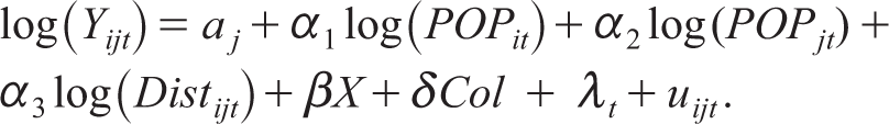
\begin{matrix} \log (Y_{i j t}) = a_{j} + α_{1} \log (P O P_{i t}) + α_{2} \log (P O P_{j t}) + \\ α_{3} \log (D i s t_{i j t}) + β X + δ C o l + λ_{t} + u_{i j t} . \end{matrix}

(3)

Here, the dependent variable Y_ijt represents the volume of migration to destination country j from the source country i during the period t. Here, the source country is fixed, that is, India, while the destination countries represented by j are the 25 sample OECD countries one by one. Term a_j captures the country fixed effect to control for the individual-level heterogeneity among the destination countries in terms of receiving the number of migrants, and λ_t captures the time fixed effect in the panel model. POP_it and POP_jt are the population of the source and destination country, respectively, at time t, Dist_it is the distance between the source country i and destination country j. In the equation, X is a vector of other important controls included in the models, namely differences in the level of per capita income, the difference in the degree of control over corruption and the difference in the level of employment. The variable col is a dummy with a value of 1 for the common official languages of both the source and destination countries and 0 otherwise. Term u_ij is the normal error term capturing the effect of all other factors on immigration not included in the model.

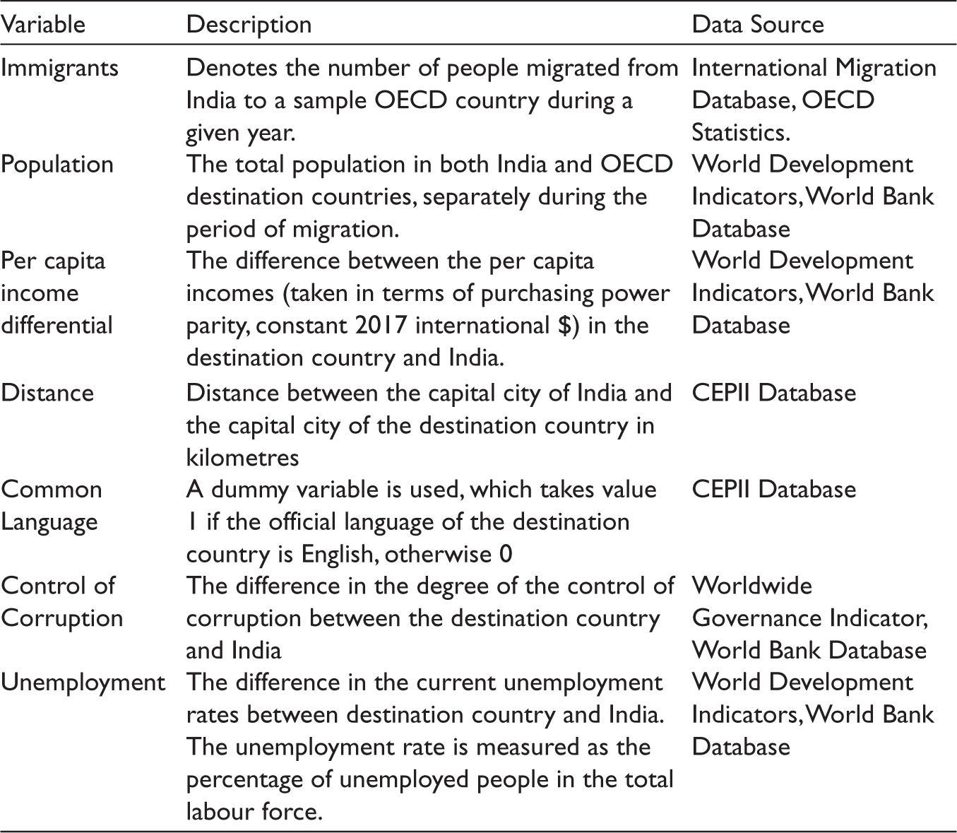
The primary data sources are the International Migration Database in OECD Statistics, World Development Indicators database, Worldwide Governance Indicator database and CEPII database. All those counties are selected in the sample for which complete data was available from 2001 to 2019. In total, there are 25 countries in the sample. Data on the population of India and OECD countries for the same period have been taken from World Development Indicators. All the used variables and their descriptions with sources are given in Table 2.

Table 2.

Variable Description and Summary Statistics.

Variable	Description	Data Source
Immigrants	Denotes the number of people migrated from India to a sample OECD country during a given year.	International Migration Database, OECD Statistics.
Population	The total population in both India and OECD destination countries, separately during the period of migration.	World Development Indicators, World Bank Database
Per capita income differential	The difference between the per capita incomes (taken in terms of purchasing power parity, constant 2017 international $) in the destination country and India.	World Development Indicators, World Bank Database
Distance	Distance between the capital city of India and the capital city of the destination country in kilometres	CEPII Database
Common Language	A dummy variable is used, which takes value 1 if the official language of the destination country is English, otherwise 0	CEPII Database
Control of Corruption	The difference in the degree of the control of corruption between the destination country and India	Worldwide Governance Indicator, World Bank Database
Unemployment	The difference in the current unemployment rates between destination country and India. The unemployment rate is measured as the percentage of unemployed people in the total labour force.	World Development Indicators, World Bank Database

Source: The authors.

First, we apply the Prais–Winsten regression with PCSE to estimate Equation 3. This method allows for possible cross-sectional correlation among the errors for different groups in the panel and takes care of resulting heteroscedasticity by providing robust estimates. Moreover, this method also takes care of first-order serial correlation (AR(1)) in the model. Some of the explanatory variables in our model may be endogenous which means that these variables are also affected by the volume of immigration (the dependent variable) or by certain migration determining factors not present in the model. The potential candidates for the endogeneity are the populations of both source and destination countries. The populations in both the source and destination countries are also subject to change owing to migration in a period. Similarly, the factors that are not included in the model but affect the volume of migration may also affect the stock of the source country’s population in the destination country. Applying the Prais–Winsten regression with PCSE in the presence of endogeneity gives biased estimates of the variables of interest.

Therefore, we check the consistency of the results obtained in the first stage by applying the instrumental variable regression model for Panel data. Specifically, we apply the two-stage least squares random effects estimator with the implementation of generalised two-stage least square (G2SLS) of Balestra and Varadharajan-Krishnakumar (1987). By assuming the populations in India and destination countries as endogenous, we use their first lags as instruments in the model. Similarly, we also apply the Hausman–Taylor estimator to take care of endogeneity.³ There are some variables in our specification which are time-invariant and remain constant within the panel. The instrumental variable regression model does not provide the estimates by distinguishing between time-variant and time-invariant variables.

The Hausman–Taylor regression allows the estimation by including the endogenous as well as time-invariant variables in the model specification. Hence, applying this model also serves as a measure to check the consistency of the results obtained in the earlier models. Another potential threat to our estimation is the presence of multilateral resistance. Bertoli and Moraga (2013) highlight that ignoring the multilateral resistance biases the estimates of migration determinants even if the migration flows are running from a single origin to multiple destinations as in the present case. They show that the primary cause of this bias in the estimates is the induced endogeneity in the regressors and serial and spatial correlation in the errors due to the presence of multilateral resistance. However, due to the limited cross-sectional and time observations, the present studies cannot employ the common correlated effect estimator of Pesaran (2006) to deal with the issues originated due to the presence of multilateral resistance. Nonetheless, the Hausman–Taylor regression technique alleviates the problem of endogeneity and, hence, can reduce the bias in the estimates up to an extent.⁴

Preliminary Analysis

Figure 1 depicts the trend of total migration from India to sample OECD countries during the sample period. Overall, it has an increasing trend, which seems to become steeper since 2016.

Figure 1.

Source: The authors.

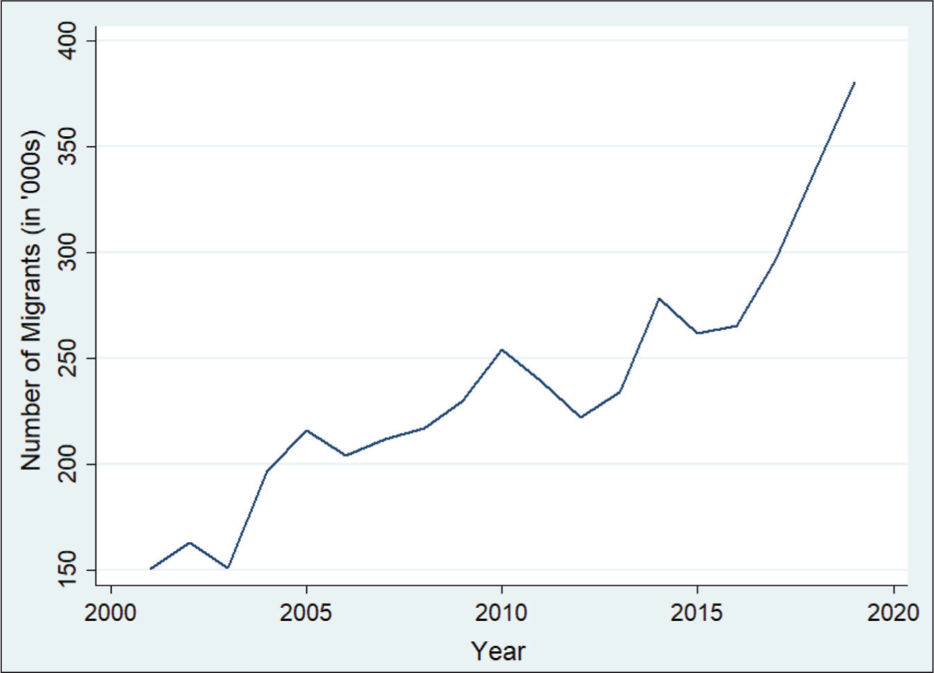
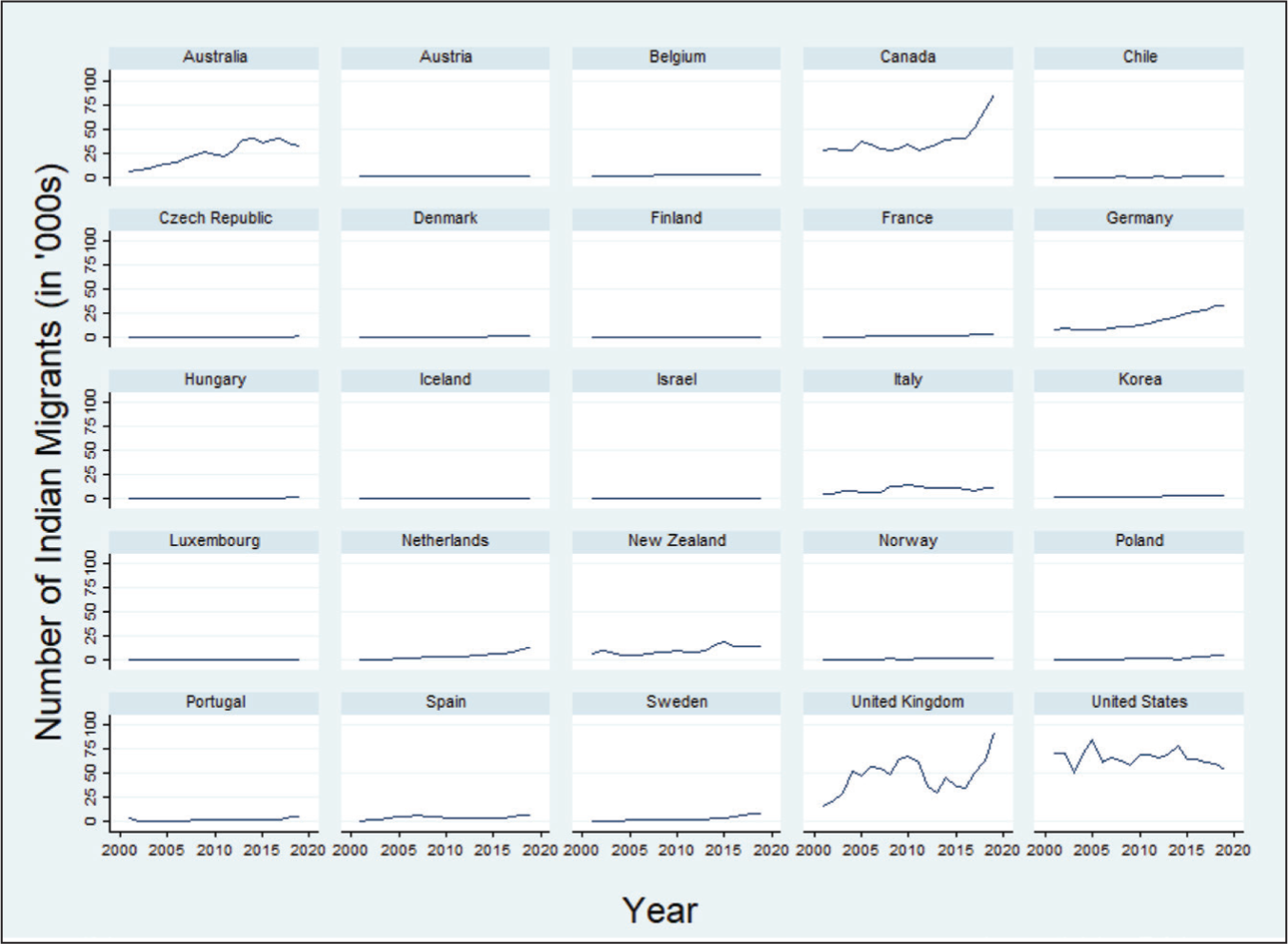
The apparent reason can be the continuous growth of the population in India during the period of study. This fact is also in accordance with our theoretical model of migration. Similarly, higher earnings in the destination countries also seem to be the driver of this increasing migration volume. However, we need to do a further appropriate regression analysis to check whether these apparent relationships hold. Figure 2 highlights the trend in migration to sample OECD countries individually. Figure 2 corroborates what is highlighted in Table 1—major receivers of Indian migrants are the United States, the United Kingdom, Canada and Australia. Despite homing a large number of migrants, the United States has a stable trend with a mild decline in recent years, possibly due to various measures and policies to curb immigration enacted in recent years under the presidentship of Donald Trump. In contrast, migrations to the United Kingdom and Canada have picked up recently due to their lenient immigration policies.⁵ Germany has also emerged as a major destination for Indian migrants, especially for students and IT professionals, in recent years. Butsch (2018) argues that the changes in German immigration policies, the launch of a green card programme for IT professionals to fill in the shortage of skilled workers in early 2000 and the internationalisation of the university system are the primary reasons for the surge in inflow of Indian migrants.

Figure 2.

Source: The authors.

Descriptive Statistics and Pairwise Correlation

Table 3 presents the descriptive statistics of the variables used in our model. The data is strongly balanced. The variable immigration has a mean value approximately equal to 9,503, which means that on average these many people migrate from India to these countries annually. But the migration has significant variability, as evident from its high standard deviation. However, the overall distribution of the variable is close to symmetric (as shown in the box plot presented in Figure B.1) despite the greater variability. Similarly, the population in destination countries and India have greater variations, but their distributions are also not very asymmetric. The variable distance, ‘Dist’, has a mean value approximately equal to 7,342 kilometres and has a high standard deviation roughly equal to 2,975 kilometres. This variable is also used in logarithmic form in the regression analysis. The difference in per capita income, ‘PCI’ is also symmetrically distributed. However, the variable ‘Unemp’ has asymmetric distributions. The distributions of all the variables are shown through the box plot in Figure B.1.⁶

Table 3.

Descriptive Statistics.

Variable	Observations	Mean	Std Dev.	Minimum	Maximum
Immigration	475	9503.116	17621.043	0.000	92,000
Pop_OECD	475	35,519,698	60,367,934	284,968	3.283e+08
Pop_India	475	1.229e+09	89,049,857	1.075e+09	1.366e+09
PCI	475	43353.409	16433.575	15122.004	113715.300
Dist	475	7342.753	2975.240	4068.379	16936.539
Lang	475	0.240	0.428	0.000	1.000
Unemp	475	1.411	3.439	–3.920	20.420
Corrupt	475	1.882	0.688	0.273	2.946

Source: The authors.

Note: In this table, the variables such as ‘Immigration’, ‘Pop_OECD’ and ‘Pop_India’ are shown in level forms. ‘Dist’ and ‘Lang’ denote Distance and Language as explained in the variable description. ‘PCI’, ‘Unemp’ and ‘Corrupt’ are the differences in the per capita income, unemployment rates and the degree of control of corruption, respectively, as defined in Table 2.

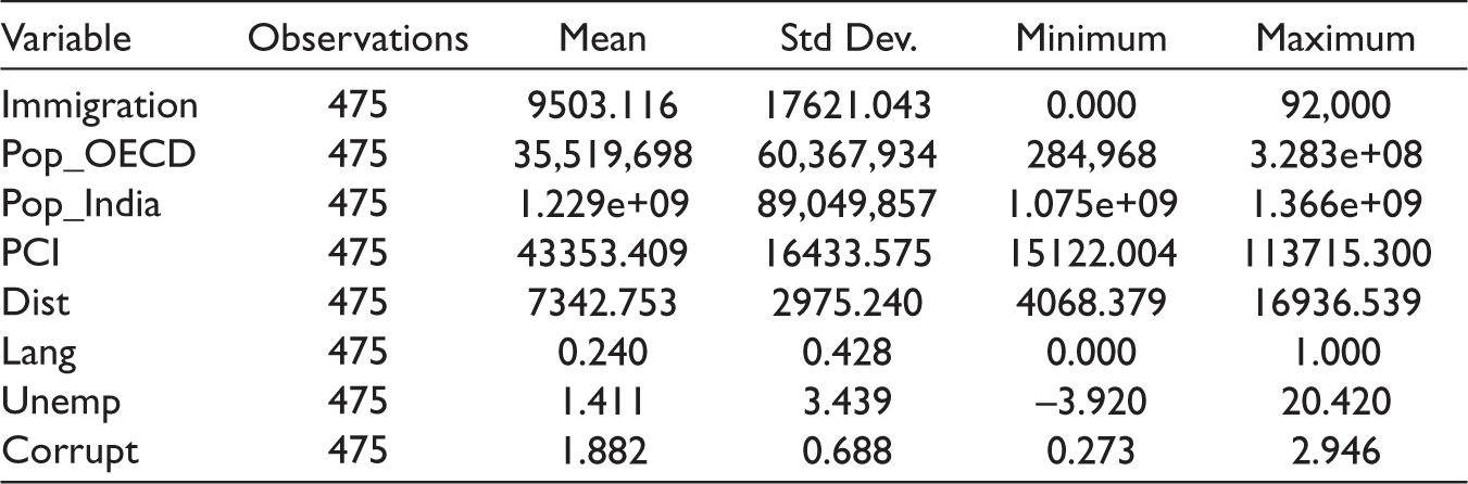
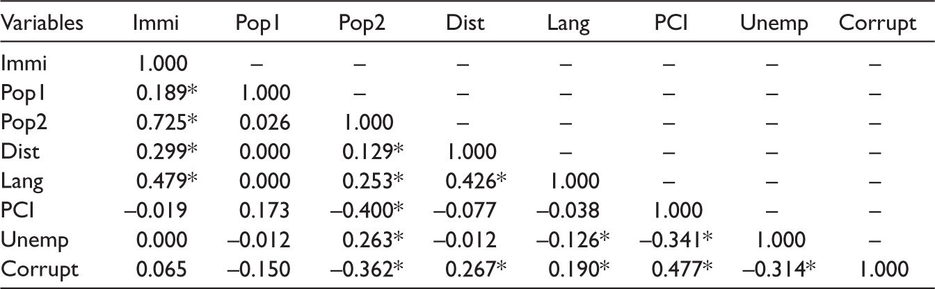
Table 4 presents the pairwise correlation among the variables used in the model. The first column reports the correlation of the migration volume with the other explanatory variables; ‘Pop1’, ‘Pop2’, ‘Dist’ and ‘Lang’ have positive association with migration volume, while the remaining variables do not have any significant correlation with migration volume. Looking at the values of correlation among the explanatory variables in the table, we can assume that our model does not suffer from multicollinearity, as the magnitude of the correlation is not very high. To further prove this, we report the variance inflationary factor (VIF) in Table A.1 after running a simple regression for the same set of variables.

Table 4.

Pairwise Correlation.

Variables	Immi	Pop1	Pop2	Dist	Lang	PCI	Unemp	Corrupt
Immi	1.000	–	–	–	–	–	–	–
Pop1	0.189*	1.000	–	–	–	–	–	–
Pop2	0.725*	0.026	1.000	–	–	–	–	–
Dist	0.299*	0.000	0.129*	1.000	–	–	–	–
Lang	0.479*	0.000	0.253*	0.426*	1.000	–	–	–
PCI	–0.019	0.173	–0.400*	–0.077	–0.038	1.000	–	–
Unemp	0.000	–0.012	0.263*	–0.012	–0.126*	–0.341*	1.000	–
Corrupt	0.065	–0.150	–0.362*	0.267*	0.190*	0.477*	–0.314*	1.000

Source: The authors.

Notes: In all the tables from here, ‘Immi’ is the log of immigration variable, ‘Pop1’ is the log of the population in India, ‘Pop2’ is the log of the population in each OECD country one by one and ‘Dist’ is the log of distance. The remaining variables are the same as defined in Table 3. ‘*’ shows significance at 5% level.

Results and Discussion

Table 5 presents the estimated results of the proposed models. The first column reports the estimates using the Prais–Winsten regression with PCSE. The estimate of the populations of the origin and destination are positive and significant at 1% level of significance, which implies that ceteris paribus, if the population of the origin (or destination) country increases, the volume of migration goes up. PCI also has a positive and significant estimate at 1% level of significance, which signifies that migration volume responds positively to the differential in the per capita incomes between destination country and India. Surprisingly, the variable distance has a positive but weakly significant estimate, which is also not in accordance with the earlier empirical evidence in some migration studies. However, more on the reliability of the estimates of distance common official language is discussed in the results of the next models. Term ‘Lang’ has a positive and significant estimate (1.049), implying that all else equal, chances of Indian migrants moving to the countries with English as an official language are approximately higher by 1% compared to moving to a country with other languages.⁷ ‘Unemp’ has a negative and significant estimate at 1% level of significance. This estimate implies that keeping everything unchanged, if the unemployment rate differential between the destination country and India increases by 1%, the immigration volume to that country goes down by 0.04%. ‘Corrupt’ has an insignificant estimate. However, all the above-discussed natures of the associations may not be true due to econometric issues present in the model discussed in the third section. Column 2 in Table 5 presents the results using the instrumental variable regression model explained in the third section. Here ‘Pop1’, ‘Pop2’, ‘Lang’ and ‘PCI’ have estimates similar to the first model. However, ‘Dist’ and ‘Unemp’ have insignificant estimates, while ‘Corrupt’ has a positive and significant estimate at the 5% level of significance, thereby implying that Indian migrants are more likely to move to those countries, which have a higher degree of control over corruption compared to India.

Table 5.

Results Using PCSE, IVREG and HTREG Models.

Variables	PCSE	IVREG	HTREG
Variables	Immi	Immi	Immi
Pop1	4.206*** (0.950)	4.546***	5.111***
	4.206*** (0.950)	(0.484)	(0.594)
Pop2	1.108*** (0.0986)	1.020***	–0.705
	1.108*** (0.0986)	(0.157)	(0.572)
Dist	0.743*	0.677	–10.15***
	(0.431)	(0.729)	(1.300)
Lang	1.049**	1.218**	6.241***
	(0.427)	(0.588)	(1.967)
PCI	0.551***	0.673***	0.730***
	(0.099)	(0.169)	(0.212)
Unemp	–0.048***	0.000	0.002
	(0.018)	(0.010)	(0.011)
Corrupt	0.197	0.237**	0.216*
	(0.139)	(0.120)	(0.128)
R-square	0.750	0.741	–
Observations	471	447	471
No. of Countries	25	25	25
Country Fixed Effect	Yes	Yes	–
Time Fixed Effect	No	No	–

Source: The authors.

Notes: All the variables are the same as explained earlier; the Hausman–Taylor model does not report the R-square. Values in parentheses are the standard errors. In all the regression results, ***, ** and * indicate the significance at 1%, 5% and 10% levels, respectively.

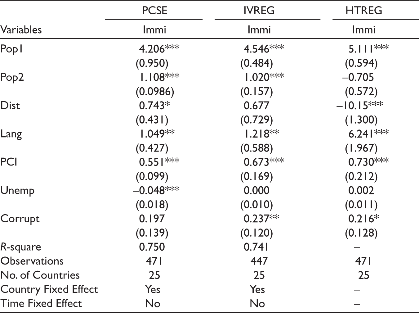
The third column presents the result of the Hausman–Taylor regression.⁸ In this model, we assume ‘Pop1’ and ‘Pop2’ as the endogenous variables as mentioned in the methodology section. Compared to the earlier two models, here ‘Pop2’, ‘Dist’ and ‘Unemp’ have different results; ‘Pop2’ and ‘Unemp’ have turned insignificant here, while ‘Dist’ has a negative and significant estimate. This negative impact of distance implies that migration volume goes down with the increase in distance between the destination and origin countries. Moreover, the estimate of ‘Corrupt’ has also become weaker than what is obtained under instrumental variable regression. Since the Hausman–Taylor model takes care of major econometric issues as discussed in the third section, we consider the results obtained here as most reliable and, hence, formulate the concluding remarks based on them. All in all, we argue that the population of the source country, distance between source and destination, common official language, and the per capita income differential between destination and source are the major determinants for the migratory movements of Indian citizens to OECD countries. Governance quality as measured through the degree of control of corruption is also another consideration of the Indian migrants. However, the population in the destination countries and the unemployment rate differential between destination countries and India are not found to be affecting the migratory flows from India.

Conclusion and Policy Suggestion

To conclude, in the present analysis, using the theoretical foundations, we investigate the impact of various economic and demographic factors on the migratory movement from India to 25 OECD countries from 2001 to 2019. Moreover, we also address the econometrics issues arising in the estimation of the gravity model of migration. Based on the findings from this analysis, we can conclude that, on the one hand, migration from developing countries to developed countries is determined by social and regional factors such as population, distance, common culture and language. On the other hand, economic factors like differences in the wage rates and employment availability also play essential roles in this process. In the present case, the source country’s population is the primary determinant of the volume of migration in the sense that a higher population in a country promotes the migration flow. In the present study, the population of the migrants’ destination country does not seem to be strongly affecting the migration flow as its estimate is not consistently significant in all models. This effect is due to two reasons. First, the theoretical postulation of the gravity model of migration about the positive impact of source and destination countries populations on migration volume considers bidirectional migration movements. Whereas, in the present case, we only consider the unidirectional migration movement. Second, a high population in the migrants’ destination country might also discourage the migratory flows through the rise in unemployment rates.⁹ The distance, in the present case, is shown to be negatively affecting the migration flow. The common official language also exhibits the desired effect on the migration flow. The difference in the per capita income between the destination and source country is positive and significant in all the models and supports the earlier evidence favouring the positive effect of relatively higher wages in the destination countries on the flow of migration. Moreover, the difference in employment rates and degree of control of corruption are also considered important determinants of migration, but they are not found to be strongly and consistently impacting the migration volume in the present study.

India has continuously been trying to decelerate the process of brain drain to the developed countries. In the backdrop of our findings in terms of per capita income, there is a need for an upward revision in the pay scale of the white-collar workers in the organised sector. We argue that their pay scale in India should be brought at par with the international standard in purchasing power parity terms to lessen the scope of them moving out due to a positive wage differential. Although not conspicuous in our case, we expect the indicators of governance and institutional qualities such as the rule of law, government effectiveness, control of corruption and quality of life like life expectancy, literacy and better health to play vital role in determining migration flows. Therefore, India must go a long way on these dimensions to meet the international standard and reduce the flow of people from the creamy layer.

There are, however, certain limitations of the present work due to the unavailability of data over various aspects that go into the determination of international migration flows. First, though the claims made in the current research are in accordance with some of the early empirical studies, they cannot be generalised and applied to migration studies of all the regions and countries with different socio-economic statuses from selected countries. Second, the small size of the chosen sample also makes the study’s claims less likely to apply to other regions. The choice of the variables also seems to shorten the scope of the study’s conclusions. A study on the migration of workers of different skill categories with varying levels of education and gender differences may give more insight into the migration process. Third, the institutional factors—such as the degree of regulatory quality, the rule of law, economic freedom and degree of financial and human development—also play a significant role, but the present study does not include all such factors barring the control of corruption.¹⁰

Therefore, this study provides the basis for more comprehensive analyses concerning the migration patterns and consequent trade relation between the developing and the developed countries. A more insightful examination of migration with more discerning impacts of its determinants can be accomplished by incorporating the dimensions of governance, institutional quality and quality of life among its determinants.

Footnotes

Declaration of Conflicting Interests

The authors declared no potential conflicts of interest with respect to the research, authorship and/or publication of this article.

Funding

The authors received no financial support for the research, authorship and/or publication of this article.

Appendices

Notes

References

Adsera

, & Pytlikova

(2015). The role of language in shaping international migration. The Economic Journal, 125(586), F49–F81.

Alimi

O. B.

, Maré

D. C.

, & Poot

(2019). Modelling inter-urban migration in an open population setting: The case of New Zealand. In Population, place, and spatial interaction (pp. 201–223). Springer.

Anderson

J. E.

(2011). The gravity model. Annual Review in Economics, 3(1), 133–160.

Anderson

J. E.

, & Van Wincoop

(2004). Trade costs. Journal of Economic literature, 42(3), 691–751.

Balestra

, & Varadharajan-Krishnakumar

(1987). Full information estimations of a system of simultaneous equations with error component structure. Econometric Theory, 3(2), 223–246.

Beine

, Docquier

, & Ozden

(2009). Diasporas. The World Bank.

Beine

, & Parsons

(2015). Climatic factors as determinants of international migration. The Scandinavian Journal of Economics, 117(2), 723–767.

Bertoli

, & Moraga

J. F. H.

(2013). Multilateral resistance to migration. Journal of Development Economics, 102, 79–100.

Biavaschi

, Burzyński

, Elsner

, & Machado

(2020). The gain from the drain: Skill-biased migration and global welfare. Journal of Development Economics, 142, 102317.

10.

Borjas

G. J.

(2003). The labor demand curve is downward sloping: Reexamining the impact of immigration on the labor market. The Quarterly Journal of Economics, 118(4), 1335–1374.

11.

Boubtane

, Coulibaly

, & Rault

(2013). Immigration, unemployment and GDP in the host country: Bootstrap panel Granger causality analysis on OECD countries. Economic Modelling, 33, 261–269.

12.

Butsch

(2018). The ‘Indian diaspora’ in Germany–emerging networks and new homes. Diaspora Studies, 11(1), 79–100.

13.

Campaniello

(2014). The causal effect of trade on migration: Evidence from countries of the Euro-Mediterranean partnership. Labour Economics, 30, 223–233.

14.

Card

(2001). Immigrant inflows, native outflows, and the local labor market impacts of higher immigration. Journal of Labor Economics, 19(1), 22–64.

15.

Chanda

, & Betai

N. V.

(2021). Implications of Brexit for skilled migration from India to the UK. Foreign Trade Review, 56(3), 289–300.

16.

Disney

, Wiśniowski

, Forster

J. J.

, Smith

P. W.

, & Bijak

(2015). Evaluation of existing migration forecasting methods and models [Report for the Migration Advisory Committee: Commissioned research]. ESRC Centre for Population Change, University of Southampton.

17.

Docquier

, Lohest

, & Marfouk

(2007). Brain drain in developing countries. The World Bank Economic Review, 21(2), 193–218.

18.

Epstein

G. S.

, & Gang

I. N.

(2006). The influence of others on migration plans. Review of Development Economics, 10(4), 652–665.

19.

Fan

, Liu

, Zhang

, & Zhang

(2018). The spatio-temporal characteristics and modeling research of inter-provincial migration in China. Sustainability, 10(3), 618.

20.

Friedberg

R. M.

, & Hunt

(1995). The impact of immigrants on host country wages, employment and growth. Journal of Economic Perspectives, 9(2), 23–44.

21.

Graves

P. E.

(1980). Migration and climate. Journal of Regional Science, 20(2), 227–237.

22.

Greenwood

M. J.

(1970). Lagged response in the decision to migrate. Journal of Regional Science, 10(3), 375–384.

23.

Hair

J. F.

Jr. , Anderson

R. E.

, Tatham

R. L.

& Black

W. C.

(1995). Multivariate data analysis (3rd ed.). Macmillan.

24.

Hausman

J. A.

, & Taylor

W. E.

(1981). Panel data and unobservable individual effects. Econometrica: Journal of the Econometric Society, 49(6), 1377–1398.

25.

Hicks

J. R.

(1932). The theory of wages. Macmillan.

26.

Jandová

, & Paleta

(2015). Gravity models of internal migration: The Czech case study. Review of Economic Perspectives, 15(1), 3–14.

27.

Kim

, & Cohen

J. E.

(2010). Determinants of international migration flows to and from industrialised countries: A panel data approach beyond gravity. International Migration Review, 44(4), 899–932.

28.

Lewer

J. J.

, & Van den Berg

(2008). A gravity model of immigration. Economics letters, 99(1), 164–167.

29.

Mamertino

, & Sinclair

T. M.

(2019). Migration and online job search: A gravity model approach. Economics Letters, 181, 51–53.

30.

Mayda

A. M.

(2010). International migration: A panel data analysis of the determinants of bilateral flows. Journal of Population Economics, 23(4), 1249–1274.

31.

Naujoks

(2009). Emigration, immigration, and diaspora relations in India. Migration Information Source. https://www.migrationpolicy.org/article/emigration-immigration-and-diaspora-relations-india

32.

OECD. (2019a). International migration and displacement trends and policies report to the G20.

33.

OECD. (2019b). Migration data brief. Migration Data Brief © OECD/AFD N°4 June 2019. https://www.oecd.org/migration/mig/Migration-data-brief-4-EN.pdf

34.

Ortega

, & Peri

(2009). The causes and effects of international migrations: Evidence from OECD countries 1980–2005 (No. w14833). National Bureau of Economic Research.

35.

Pesaran

M. H.

(2006). Estimation and inference in large heterogeneous panels with a multifactor error structure. Econometrica, 74(4), 967–1012.

36.

Prais

S. J.

, & Winsten

C. B.

(1954). Trend estimators and serial correlation (Cowles Commission Discussion Paper No. 383, pp. 1–26). University of Chicago.

37.

, Zhao

, Chi

, Zhao

, & Kong

(2019). A spatial dynamic panel approach to modelling the space-time dynamics of interprovincial migration flows in China. Demographic Research, 41, 913–948.

38.

Rajesh

(2018). Assessing the impact of great recession on India’s trade in gravity model framework. Foreign Trade Review, 53(4), 239–270.

39.

Ramos

(2016). Gravity models: A tool for migration analysis. IZA World of Labor.

40.

Ravenstein

E. G.

(1885). The laws of migration. Journal of the Statistical Society of London, 48(2), 167–235.

41.

Ringle

C. M.

, Wende

, & Becker

J.-M.

(2015). SmartPLS 3. SmartPLS.

42.

Tinbergen

(1962). Shaping the world economy: Suggestions for an international economic policy. Twentieth Century Fund.

43.

Zimmer

(2008, June). Network effects on domestic migration flows across Germany: A spatial autoregressive perspective with spatially structured origin and destination effects and heteroskedastic innovations. In Seventh workshop on spatial econometrics and statistics, Paris (pp. 9–10). http://www.nzae.org.nz/wp-content/uploads/2011/08/nr1215391007.pdf