
Abstract
Based on input/output tables that contain disaggregated data from 45 industries grouped into 16 sectors from 1995 to 2020 across 66 countries, we carry out a gravity analysis to examine how imported inputs affect bilateral exports. In terms of econometric methodology, we use pseudo Poisson maximum likelihood (PPML) as well as Instrumental-Variable Tobit methods. Our results consistently show a positive and significant effect of imported inputs on bilateral exports.
Introduction
According to the World Trade Organization (WTO), the share of intermediate inputs in total trade (excluding fuels) has consistently hovered around 50% for the last 10–15 years or so. 1 Furthermore, trade in intermediate inputs takes place even at a larger scale and for a longer period among the OECD (Organization of Economic Cooperation and Development) countries, and it has been between 56% and 73% of overall trade flows in goods and services since the early 1990s (Miroudot et al., 2009). The United States stands tall in this respect, with nearly 90% of its imports being capital goods, and it has witnessed its total imports soar to a staggering $2.5 trillion in 2019. 2 Imports of capital goods usually play an essential role in enhancing economic growth, as revealed by numerous scholars, including the recent work of Cavallo and Landry (2018) and Roy (2020).
Theoretical research on the economics of the international trade of intermediate inputs started with the seminal works by Baldwin (1966) and the collaborative efforts of Ronald Jones and his co-authors (Findlay and Jones, 2001; Sanyal and Jones, 1982; Jones, 2000). More recently, Eaton and Kortum (2001) extended the theory to conduct empirical studies on the topic in a more systematic way.
Since the 1980s, a lot of empirical work has shown the importance of imports of intermediate inputs for domestic factors (e.g., innovation, productivity, employment, and sales). However, not all results are positive. On one side, Van Biesebroeck (2003) found that there is no productivity improvement for Columbia firms by using imported inputs. Muendler (2004) also found that the use of foreign inputs plays a negligible role in enhancing the productivity of Brazilian firms. On the other side, using cross-country data for the period of 1960–1985, Lee (1995) found that imported capital goods tend to have a higher productivity than domestically produced capital goods. Hummels et al. (2001) showed that the use of imported inputs in producing goods that are exported accounted for 30% of the growth in exports. Eaton and Kortum (2001, 2002) also connected trade in intermediate inputs to productivity differences and technological progress. Amiti and Konings (2007) showed that imported intermediate inputs can raise productivity via quality effects. Kasahara and Rodrigue (2008) used firm-level panel data to analyse the effects of imports of intermediate inputs on productivity via technology transfer. Goldberg et al. (2010) analysed the role of imported intermediate inputs in promoting the introduction of new products. They found that the access of new imported intermediate inputs played a significant role in the growth of new products. Ge et al. (2011) revealed that input tariff cuts – an enhancer of intermediate imports-boost domestic productivity through learning, variety and quality channels. Kasahara and Lapham (2013) found complementarity in final good exports and intermediate imports in enhancing firm performance. Yu (2015) revealed that lower input tariffs improve productivity for processing-trade and non-processing-trade Chinese firms. Bas and Strauss- Kahn (2015) revealed significant quality upgrades due to reductions in Chinese input tariffs. Acharya and Keller (2009) and Halpern et al. (2015), using micro firm-level data, highlight the importance of imports of intermediate inputs for productivity and exports. Feng et al. (2016) uncovered that firms that expand their intermediate input imports raise the volume of their exports and increase their export scope. Liu and Qiu (2016) investigated the direct effects of intermediate input imports on innovation based on firm-level data.
It is important to not only analyse the impact of intermediate imports on factors such as innovation, productivity, employment, and sales, but also on export performance to comprehensively understand the dynamics of economic inter-connectedness and competitiveness in global markets. Bas (2012) showed that Argentine firms in industries experiencing larger input tariff reductions have a higher probability of entering the export market. Chevassus- Lozza et al. (2013) discovered that lowering input tariffs increases the export sales of high-productivity firms at the expense of low-productivity firms. Using French data, Bas and Strauss-Kahn (2014) found that using more varieties of imported input results in higher total factor productivity (TFP) and a larger scope for exports. Feng et al. (2016) found that imports of intermediate inputs significantly positively impact international exports.
In line with the literature elaborated above, India presents a good illustration of how imported intermediate inputs can drive domestic factors and export performance. 3 Until 1970 almost all computers in India were imported. In 1972, India decided to become self-reliant in computer production. It introduced high tariffs on imports of computer hardware. IBM left India within months. Electronic Corporation of India Limited was handed monopoly power by the Government of India to produce computers. Software production remained low because Indian programmers could not excel with low-quality hardware. In 1991, computer tariffs were reduced, and software production and exports skyrocketed. Similarly, Indian pharma companies produce 60% of the world’s vaccines and 20% of generic medicines. India exports pharmaceutical products to over 200+ countries. India’s market share of generics is over 50% in Africa, 40% in the USA, and 25% in the UK. India supplies 60% of global vaccines. Exports of drugs and pharma products were $24.6 billion in 2021–22 and $24.4 billion in 2020–2021. The Indian pharma industry witnessed a growth of 103% during the period 2014–2022: $11.6–$24.6 billion. Such high growth was possible in part by liberalised policies for Foreign Direct Investment (FDI). 100% FDI is allowed in the pharmaceutical sector. But, more importantly, Allowing cheap imports (mainly from China) of chemical intermediate inputs for pharmaceutical firms has helped India to be an efficient producer of pharmaceutical products. India’s imports from China of Organic chemicals went up from $5 billion in 2013 to $12 billion in 2021.
However, most, if not all, related papers analysed the impact of intermediate imports on export performance within an industry/sector. Francois and Woerz (2008) analysed the impact of services on export and value-added of the manufacturing sector. Our paper is more comprehensive as we use intermediate imports from sixteen sectors as potential drivers of export performance in sixteen sectors. Furthermore, we use bilateral trade data. 4 Our paper utilises input-output data to thoroughly examine the influence of intermediate imports from various sectors on the export performance of various sectors.
Moreover, most of the papers discussed above use firm-level or product-level data to establish a relationship between imports of intermediate inputs and productivity, growth, and exports. However, there is also room for studies using more aggregated country-level data. Micro and macro studies are not necessarily substitutes, but they typically are used to analyse different models (Magnus & Vasnev, 2008). In this article, we use bilateral trade data, and our empirical analysis is based on input/output tables from OECD that contain disaggregated data from 45 industries grouped into 16 sectors from 1995 to 2020 across 66 countries.
We employ the state-of-the-art gravity model that is known for higher predictive power. In line with recent developments in the related literature, we estimate our equations in a multiplicative form by the pseudo Poisson maximum likelihood (PPML) method as suggested by Santos Silva and Tenreyro (2006). We include in our regressions a part from customary time-varying gravity variables (i.e., trade agreements, Linder effects, and border effects), multilateral resistances (Anderson & van Wincoop, 2003), and pairwise fixed effects. These pairwise fixed effects perfectly capture all the bilateral trade costs (Agnosteva et al., 2014; Baier & Bergstrand, 2007; Egger & Nigai, 2015). These high-order fixed effects (i.e., country-time and pairwise) account for all the general equilibrium theory-consistent direct and indirect effects in international trade (Baldwin & Taglioni, 2006; Yotov et al., 2016). While pairwise fixed effects can address potential endogeneity issues arising from observable and unobservable omitted variables, we also use the IV-TOBIT estimation method to control potential simultaneity bias. Moreover, We use continuous panel data to take advantage of all available information and address potential incidental parameter bias Egger et al. (2019). We also use the method suggested by Weidner and Zylkin (2021) to address potential incidental parameter bias due to the high number of regressors in our estimations.
Our findings show, and confirm findings in many earlier empirical studies, that importing intermediate goods enhances the export performance of domestic sectors. Our results also indicate the potential phasing-out effects of intermediate imports on domestic sectors. The positive impact of intermediate imports is a potential consequence of lower production costs through the heightened competition in input markets due to imported intermediate goods. Technological progress, strategic diversification, and substitution with domestic inputs could drive the potential phasing-out effects.
Section 2 presents the data and elaborates on the methodology, Section 3 reports the empirical results, and Section 4 concludes.
Data and Methodology
Data
Our empirical analysis will be based on input/output tables from OECD (2023) that contain disaggregated data from 45 industries grouped into 16 sectors from 1995 to 2020 across 66 countries (38 OECD and 28 non-OECD countries). 5 We construct export sector-specific (d) export variables from the original input/output tables (Xdijt) from exporting countries i to importing countries j in periods t. Our export variables contain international and intra-national data. We construct country-time-specific intermediate import variables from each sector’s input/ output tables. Aggregating import variables from the disaggregated (by industry) to the aggregated one (by country) captures potential intra-industry or intra-sector relationships. Not using import variables disaggregated at the same level as the dependent variable also mirrors the fact that it might not be rational to assume that a country will be involved, simultaneously and significantly, in imports and exports of less-differentiated goods.
Percentages of production used as intermediate inputs in producing sectoral goods vary across sectors but are relatively stable from 1995 to 2000 (changes between –4.99% and 4.99% in 97% of cases). Noticeable changes include the decline in using mining as intermediate goods in producing chemicals (–29.14%), metals (–7.23%), and electric and gas (–12.66%); the increasing intra-sector dependencies in the mining, textile, electronics, electricity & gas, and water supply sectors; and the decline in the percentage of final good consumption of textile, electronics, and water supply.
Numerous potential reasons could be used to justify these noticeable trends, such as, but not limited to, technological advancements, increasing awareness of environmental issues, global economic factors, supply chain efficiency, specialisation and outsourcing, economies of scale, circular economy, and infrastructure development. However, this analysis solely focuses on the impact of intermediate goods on export performance from various sectors (e.g., agriculture, mining, food, textile, wood, paper, chemicals, plastics, minerals, and metals).
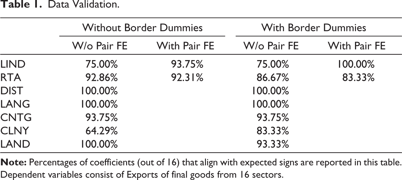
To validate our constructed dataset, we regress our dependent variables on customary gravity variables. These variables (e.g., trade agreements, geographic distance, language similarities, contiguity, colonial links, and landlockedness) are either obtained or constructed from information available on the Centre d’Études Prospectives et d’Informations Internationales (CEPII). Different researchers contributed to this database. Melitz and Toubal (2014) constructed language variables, and Mayer and Zignago (2011) provided the remaining gravity variables. Head et al. (2010) generated the original dataset containing trade agreements and colonial links variables.
The Free trade agreements (FTA ijt ) variable takes the value 1 if countries i and j are members of the same Free trade agreement in period t, and zero otherwise.
The Linder term (LIND ijt ) is computed as follows: [ln(Yit) – ln(Yjt)] 2 , with Y denoting the GDP per capita, as retrieved from World Bank (2017). This variable captures differences in the qualities of demanded goods across trading partners.
Geographic distance (DIST ij ) stands for the log of bilateral geographic distances between trading partners’ capital cities. This variable captures transportation costs to export goods from country i to country j.
We use the Common Official Language (LANG ij ) variable to capture language similarities. This dummy variable takes the value of 1 when the trading partners use similar official languages and 0 otherwise.
The contiguity (CNTG ij ) variable takes 1 (0) when the trading partners are (are not) contiguous.
Colonial links (CLNY ij ) is a dummy variable taking the value of 1 when the trading partners have ever been in a colonial relationship.
Landlockedness (LAND ij ) is a dummy variable taking the value of 1 when at least one of the trading countries is landlocked. 6
According to the results reported in Table 1, the majority of coefficients (>60%) align with estimates available in the related literature, regardless of whether we include border dummies or not. These border dummies take the value of 1 when i ≠ j and 0 otherwise.
Data Validation.
Methodology
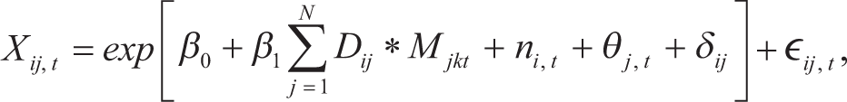
To reach the goal of this study, we augment the theory-consistent gravity equation with intermediate import variables Mjt. The gravity equation was theoretically derived by Anderson and van Wincoop (2003):
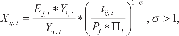
where Xij,t denotes the value of exports from country i to country j at time t, Ej,t is the total expenditure in the destination country j at time t, Yi represents the sales of goods by origin country i at time t at destination prices, and Yw,t is the world output at time t. Pj,t and Π
i,t
represent inward and outward multilateral resistances, respectively, tij,t denotes trade frictions between i and j at time t, and σ is the elasticity of substitution between the different varieties. This equation can be used to obtain theory-consistent general equilibrium estimates. The estimable augmented version of Equation (1) is given by
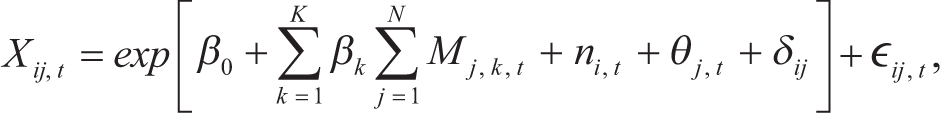
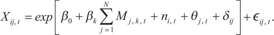
where Xi,j,t represents the exports from country i to country j from a given sector, in period t. This equation is estimated for each sector k (e.g., agriculture, food, wood, textile, paper, chemicals, minerals, metals, machinery, and services). Imports of intermediate goods from all the N partners -Mj,k,t- capture import penetration and will be used to unveil the contemporaneous impacts of imported intermediate goods on export performance. This variable is aggregated at the country-sector level (j, k) to capture the fact that domestic sectors undergo import pressure from all the trading partners and sectors at the same time. While including all the sector (K) related import variables at the same time in 2 would reflect the simultaneous impacts from all the sectors, those import variables seem to be highly correlated. Thus, we will have to alternate import variables and use one import variable at a time, as shown in the following equation:
We will consider, as regressors, sectors whose at least 1% of production was used as intermediate goods in a given sector. For instance, 34.65%, 14.11%, 2.40%, 1.80%, and 1.06% of agricultural production are considered intermediate goods in producing food, agricultural products, wood, textile, and chemicals, respectively. 7 Final agricultural product exports are regressed on intermediate imports from the food, agriculture, wood, textile, and chemicals sectors. We will select, for other sectors, intermediate imports to use as regressors in the same manner.
We use exporter-time (ni,t) and importer-time (θj,t) fixed effects to capture multilateral resistances. These multilateral resistances prevent the omission bias coined as the “gold medal mistake” by Baldwin and Taglioni (2006) committed by thousands of existing studies. These multilateral resistances account for direct as well as indirect effects in international trade and capture the general equilibrium effects of trade-policy changes (Yotov et al., 2016). More specifically, these multilateral resistances capture the fact that trade between location i and location j is influenced by variables such as prices in other locations of the world, and these prices are influenced by bilateral distances between locations i and j on the one hand with the other market locations on the other (Baier & Bergstrand, 2007).
δij denotes the exporter-sector-importer fixed effects (or, pairwise fixed effects). These fixed effects deal with endogeneity given that the dependent variable and other explanatory variables can depend on some unobservable or omitted variables (Agnosteva et al., 2014; Baier & Bergstrand, 2007; Egger & Nigai, 2015; Yotov et al., 2016). Endogeneity could also be caused by simultaneity bias, given that the productivity of foreign firms could lead to higher import exposure for domestic economies. These pairwise fixed effects thoroughly control for bilateral trade costs and will strip out all the bilateral time-invariant observable variables (e.g., geographic distance, common languages, colonial links, contiguity, and landlockedness). ϵ ij,t is the error term.
However, it is impossible to identify import variables in the presence of multilateral resistance variables. Therefore, we take advantage of the identification strategy proposed by Heid et al. (2017) and Beverelli et al. (2018) and multiply the import variable by a dummy variable Dij which takes the value 1 if i ≠ j and 0 if i = j. Thus, the equations to estimate becomes:
Estimations are performed in a multiplicative form by applying the PPML method. This method has the merit of incorporating zero export values that would be excluded if we used the OLS method to estimate a log-linearised gravity equation. It also addresses the issue of the heteroscedastic error terms created by the log transformation of the gravity model (Santos Silva & Tenreyro, 2006).
Empirical Results
In this section, we present our findings employing diverse specifications. Instead of utilising interval data as recommended by Cheng and Wall (2005), we adhere to the approach of Egger et al. (2022) by employing continuous panel data. This choice allows us to leverage the available data fully and address the potential incidental parameter bias, which can emerge due to a larger number of regressors. As elucidated in the preceding section, we incorporate only one intermediate import variable as a regressor across all regressions due to the substantial correlations among these variables. As a result, the regressors (i.e., intermediate import variables) are listed in rows, while the dependent variables (i.e., exports in final goods) are listed in columns. From an aggregate input-output table, only sector-related variables that represent at least 1% of a given sector’s production. The rationale behind the selection criteria is to focus the analysis on sector-related variables that significantly impact a given sector’s production, thereby ensuring relevance and efficiency in the research. Thus, for instance, intermediate imports in Agriculture, chemicals, food, and services are alternative explanatory variables for exports in food, while only intermediate imports in construction and services are explanatory variables for exports in construction.
Our first set of results reported in Table 2 includes exporter-time and importer-time fixed effects and other customary time-varying gravity variables (RTAijt, LINDijt, and INTijt). Out of the 95 coefficients of significant coefficients, a noteworthy 88 percent exhibit a positive orientation, indicative of the propensity for enhanced domestic producer performance by importing intermediate goods. This phenomenon is underscored by heightened competition within input markets, consequently reducing domestic production costs. Within this array of significant estimates, it is notable that imports of intermediate goods exert a contrary influence on the export performance of mining and water supply sectors.
Effects of Intermediate Imports on Final Goods Exports (PPML estimations without Pairwise Fixed Effects).
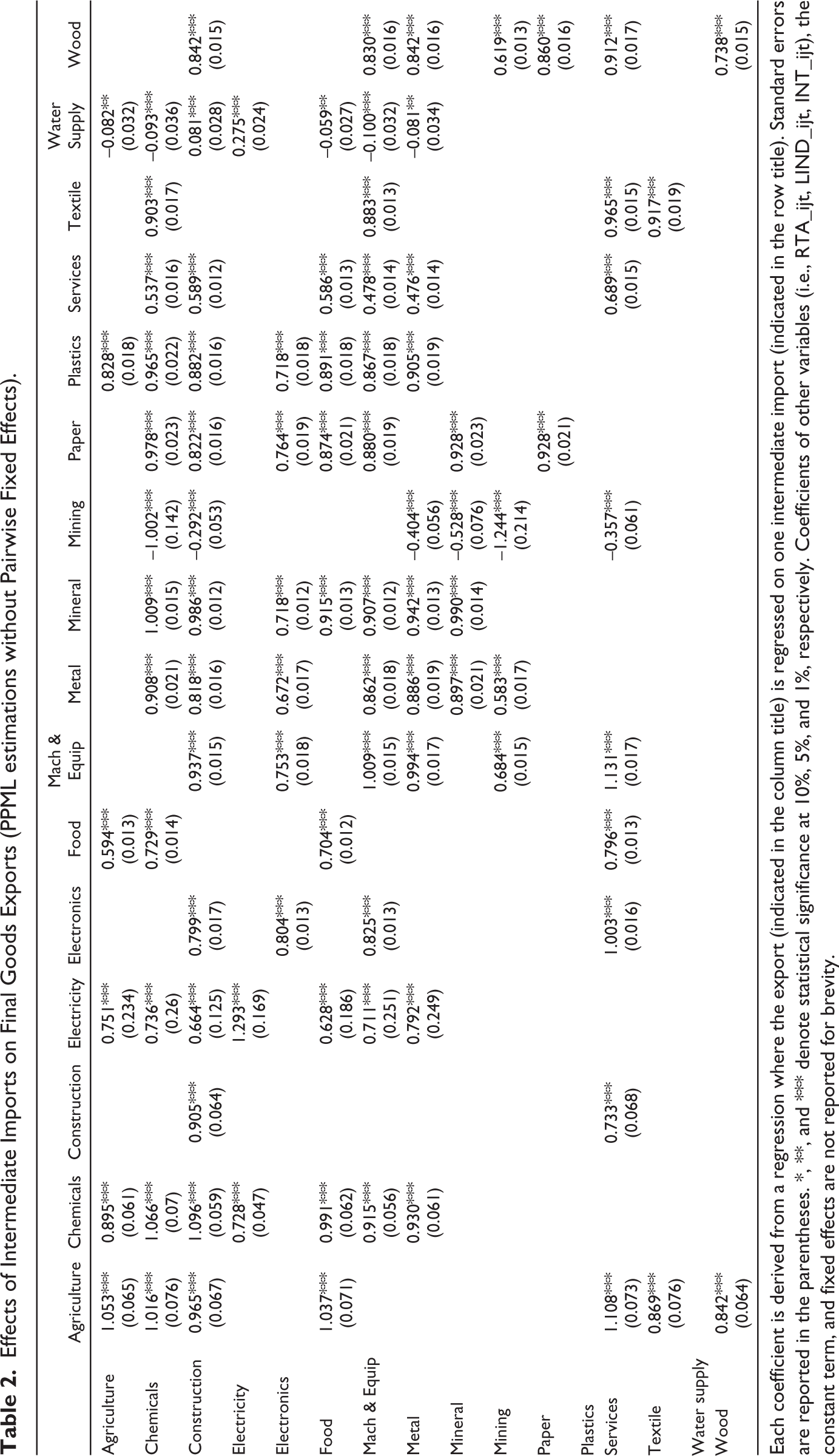
Each coefficient is derived from a regression where the export (indicated in the column title) is regressed on one intermediate import (indicated in the row title). Standard errors are reported in the parentheses. *, **, and *** denote statistical significance at 10%, 5%, and 1%, respectively. Coefficients of other variables (i.e., RTA_ijt, LIND_ijt, INT_ijt), the constant term, and fixed effects are not reported for brevity.
However, there is a potential for simultaneity bias as increases in exports may lead to higher demand for imported inputs while importing more inputs can enhance export capabilities. Thus, we mitigate this potential bias by also using the IV-TOBIT with fixed effects and considering imports of intermediate inputs as an endogenous variable. We use lagged intermediate imports as instruments for contemporaneous intermediate imports. The outcomes stemming from this analytical strategy are presented in Table 3. Accordingly, a substantial proportion of 88.42% of coefficients maintains congruence in directionality and statistical significance compared with the findings outlined in Table 2. Notably, none of the 95 significant coefficients exhibit negative values within the context of these novel outcomes.
Effects of Intermediate Imports on Final Goods Exports (IV-TOBIT Estimations Without Pairwise Fixed Effects).
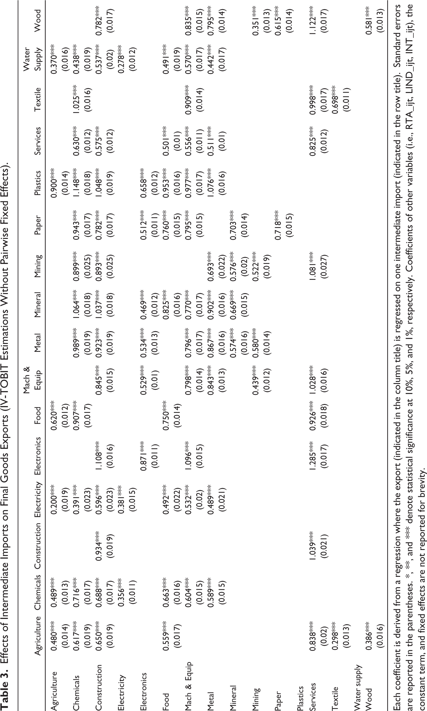
Each coefficient is derived from a regression where the export (indicated in the column title) is regressed on one intermediate import (indicated in the row title). Standard errors are reported in the parentheses. *, **, and *** denote statistical significance at 10%, 5%, and 1%, respectively. Coefficients of other variables (i.e., RTA_ijt, LIND_ijt, INT_ijt), the constant term, and fixed effects are not reported for brevity.
To comprehensively address plausible alternative origins of endogeneity and incorporate time-invariant bilateral trade costs, we employ the PPML method with three-way fixed effects (i.e., exporter-time, importer-time, and pairwise). The outcomes documented in Table 4 affirm the discernible influence exerted by the inflow of intermediate goods imports upon the operational efficacy of indigenous producers. Among the 87 statistically significant coefficients, only one is negative. Imports of intermediate agricultural goods emerge as a dampening factor upon the export trajectory of the domestic chemicals sector.
Effects of Intermediate Imports on Final Goods Exports (PPML Estimations with Pairwise Fixed Effects).
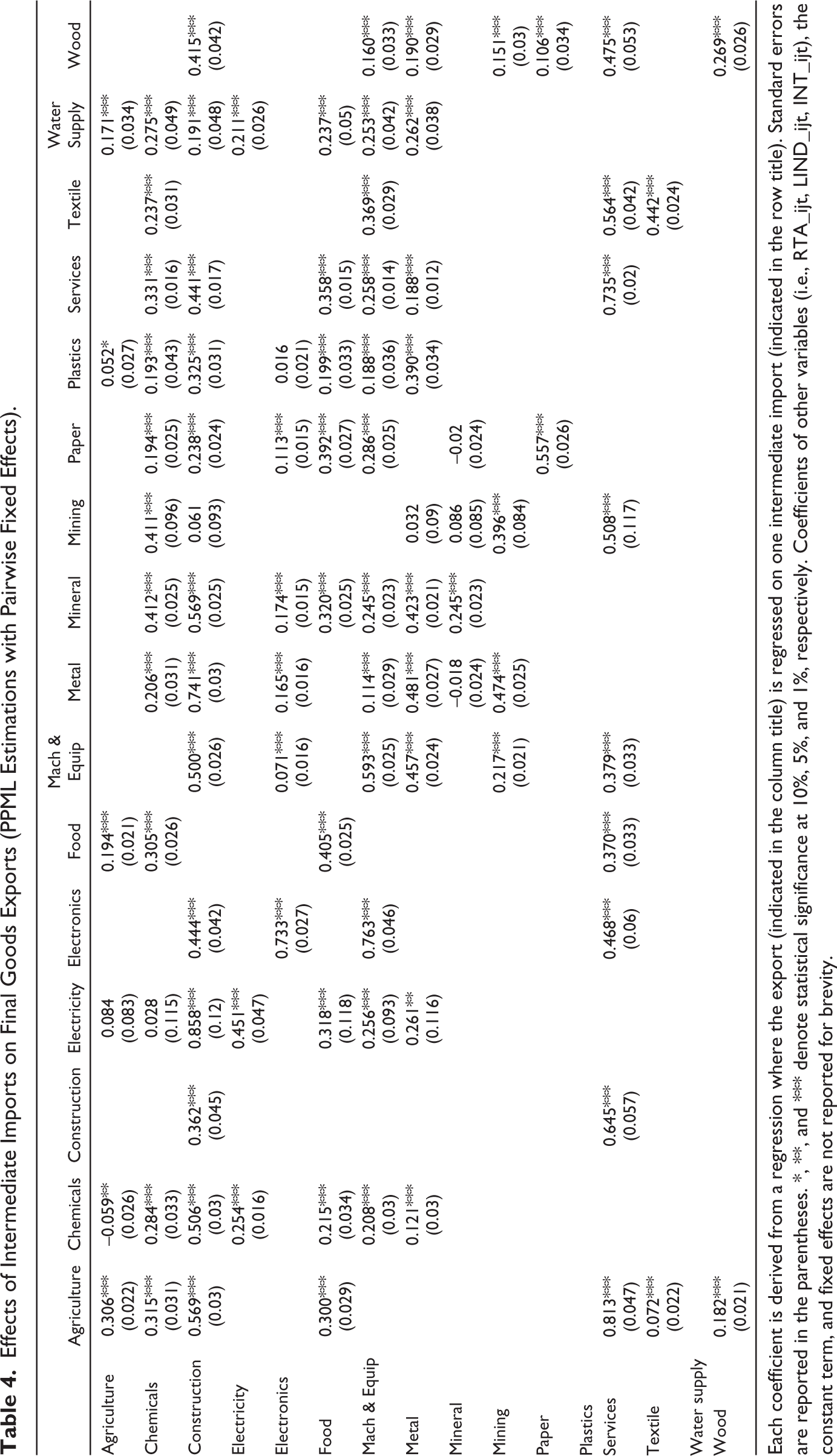
Each coefficient is derived from a regression where the export (indicated in the column title) is regressed on one intermediate import (indicated in the row title). Standard errors are reported in the parentheses. *, **, and *** denote statistical significance at 10%, 5%, and 1%, respectively. Coefficients of other variables (i.e., RTA_ijt, LIND_ijt, INT_ijt), the constant term, and fixed effects are not reported for brevity.
Before we attempt to provide an intuitive explanation for some of the coefficients, especially those deviating from our underlying assumption, we exclude INTijt variable and compare the new results to those in Table 4. As reported in Table 5, all the 95 significant coefficients are positive.
Effects of Intermediate Imports on Final Goods Exports (PPML Estimations With Pairwise Fixed Effects, Without INT–ijt).
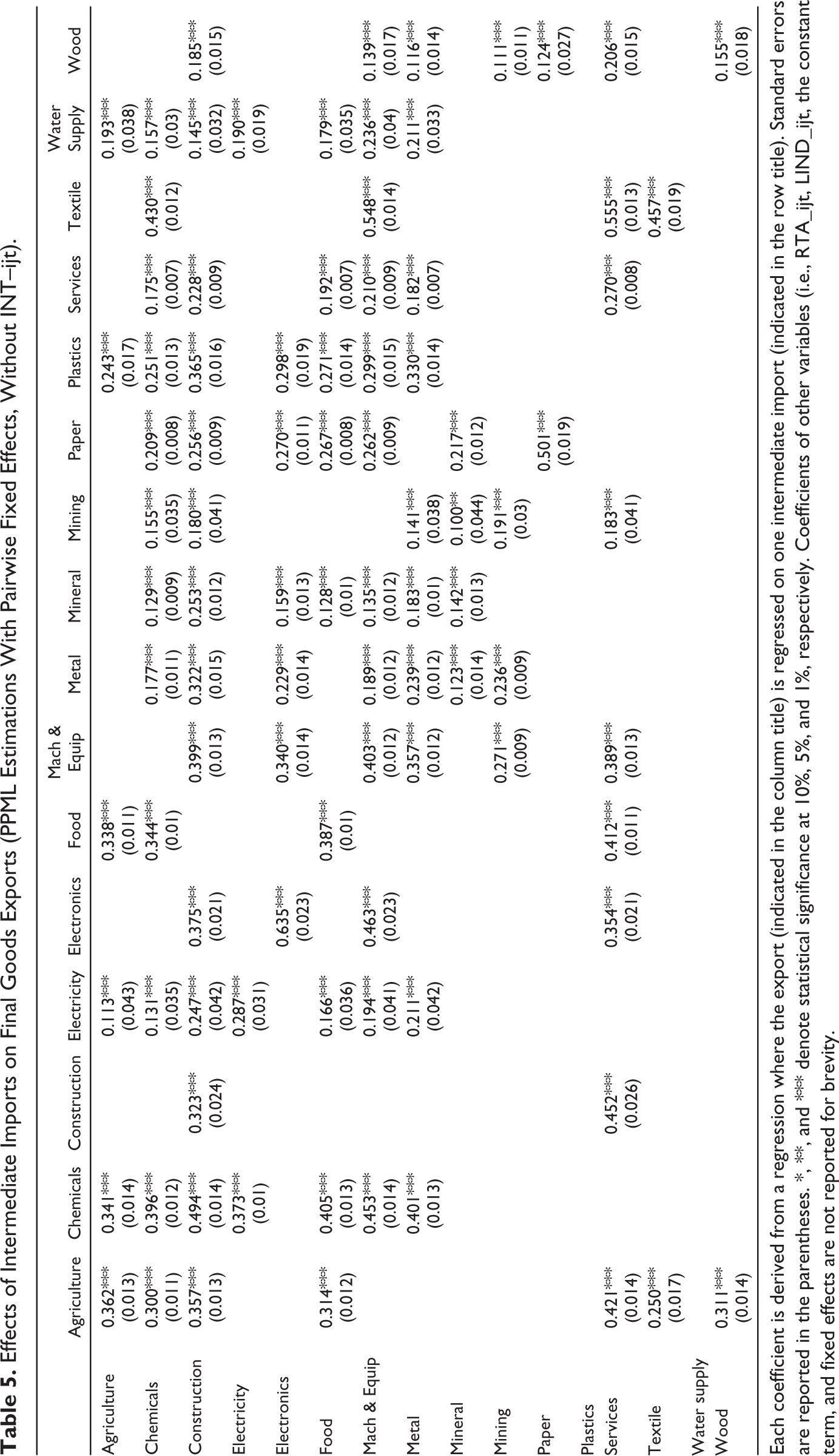
Each coefficient is derived from a regression where the export (indicated in the column title) is regressed on one intermediate import (indicated in the row title). Standard errors are reported in the parentheses. *, **, and *** denote statistical significance at 10%, 5%, and 1%, respectively. Coefficients of other variables (i.e., RTA_ijt, LIND_ijt, the constant term, and fixed effects are not reported for brevity.
Given the number of fixed effects variables included in the regression and although we use continuous panel data, it is possible that our estimates presented so far suffer from incidental parameter bias as described in Weidner and Zylkin (2021). Thus, we apply the method suggested by these authors to address potential Incidental Parameter Bias. We could notice a reduction in the number of significant coefficients (about 34.7%). Nevertheless, the underlying trend persists as all 62 statistically significant coefficients are positive, reaffirming the pivotal role that imports of intermediate goods continue to play across domestic sectors. For instance, construction exports are positively impacted only by imports of intermediate services, food exports are enhanced by imports of intermediate food and chemicals, and metal exports are enhanced by imports of intermediate electronics and machinery & equipment. Intermediate imports do not significantly boost electricity and water supply exports.
So far, we have used only contemporaneous intermediate import variables. We now modify our specification that produced Table 6 results by employing lagged intermediate import variables. It should be noted that lagged variables are highly correlated with contemporaneous ones. Thus, using them together would produce less reliable estimates. Using lagged intermediate imports as regressors will allow us to confirm the overall findings and depict potential phasing-in or phasing-out effects of intermediate imports on export performance. 77.63% of the results in Table 7 align with those from Table 6 (in sign and statistical significance). 81.94% of the positive coefficients are lower (in magnitude) than their counterparts from Table 6, thus reflecting the potential phasing out effects of intermediate imports. These apparent phasing-out effects could be due to numerous factors such as, but not limited to, technological progress, strategic diversification, substitution with domestic inputs, market dynamics, and learning curves.
Effects of Intermediate Imports on Final Goods Exports (IPP Corrected PPML Estimations With Pairwise Fixed Effects, Without INT–ijt).
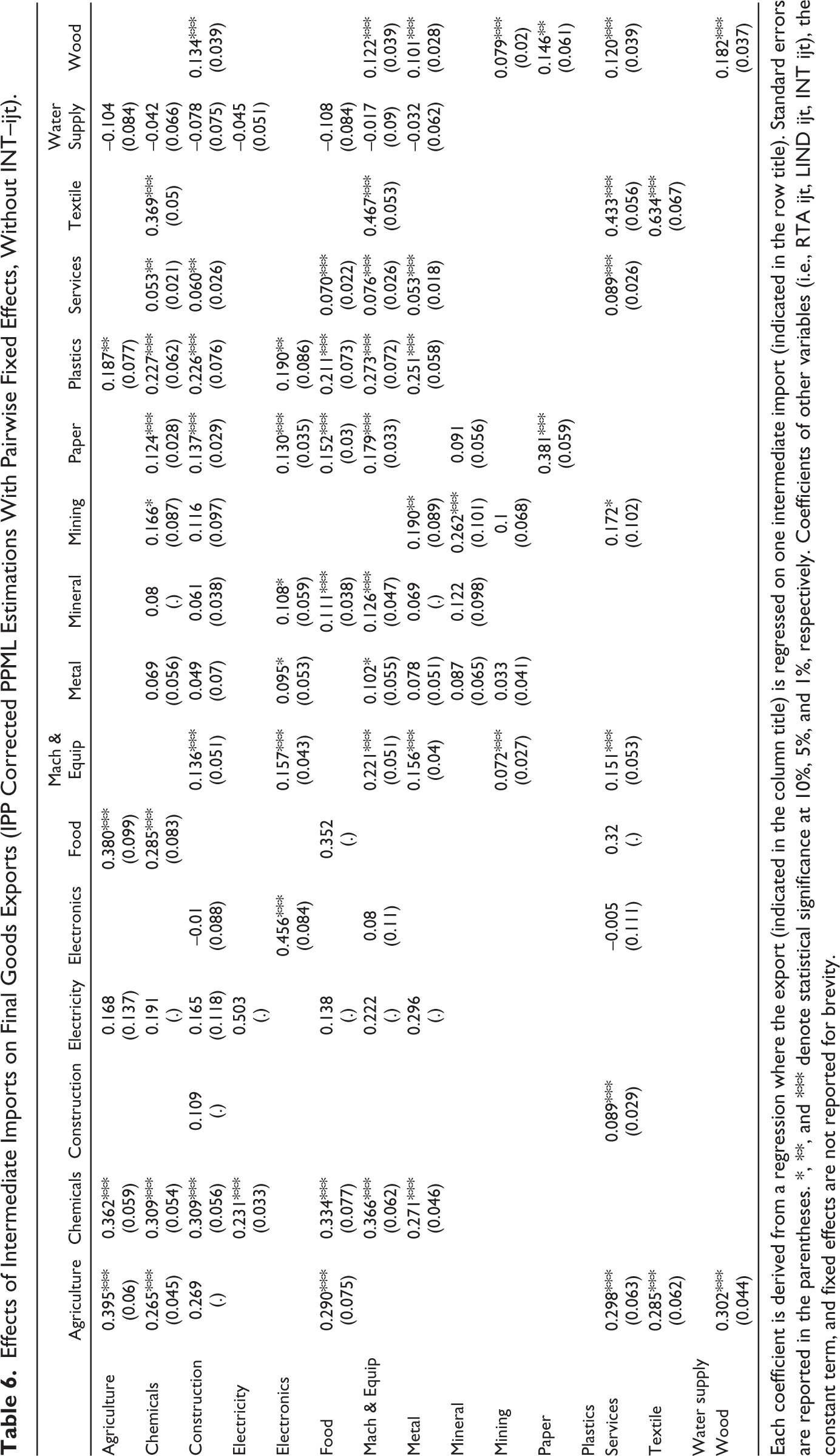
Each coefficient is derived from a regression where the export (indicated in the column title) is regressed on one intermediate import (indicated in the row title). Standard errors are reported in the parentheses. *, **, and *** denote statistical significance at 10%, 5%, and 1%, respectively. Coefficients of other variables (i.e., RTA ijt, LIND ijt, INT ijt), the constant term, and fixed effects are not reported for brevity.
Effects of Lagged Intermediate Imports on Final Goods Exports (IPP Corrected PPML Estimations with Pairwise Fixed Effects, Without INT–ijt).
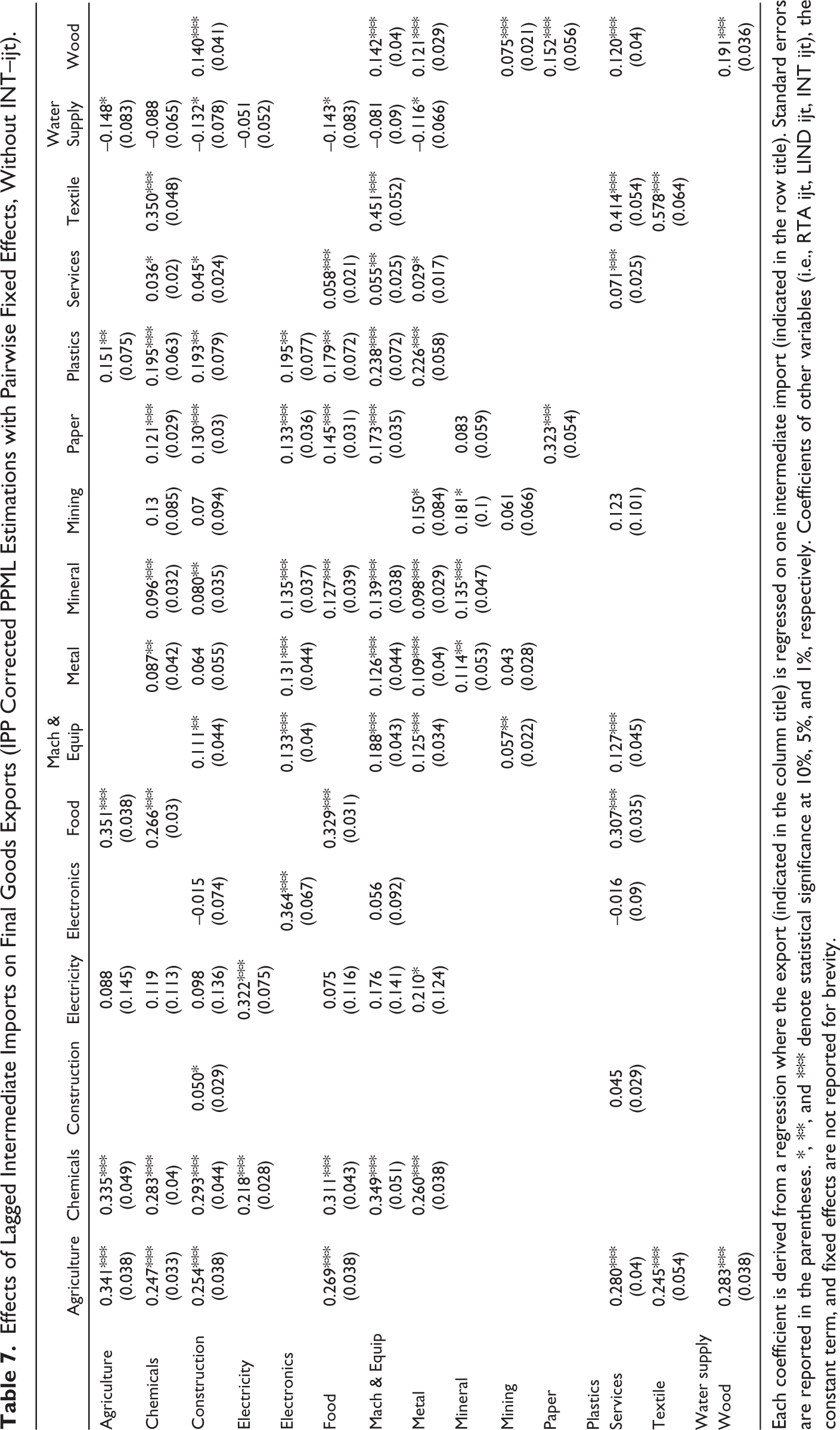
Each coefficient is derived from a regression where the export (indicated in the column title) is regressed on one intermediate import (indicated in the row title). Standard errors are reported in the parentheses. *, **, and *** denote statistical significance at 10%, 5%, and 1%, respectively. Coefficients of other variables (i.e., RTA ijt, LIND ijt, INT ijt), the constant term, and fixed effects are not reported for brevity.
The lessons from this study should serve as a warning to all countries. For instance, the Indian 2023 budget has seen new trade restrictions on imports of electronic items, imitation jewelry, chemicals, umbrellas, etc. In the 2021–2022 budget, targets of tariffs were cotton, ethyl alcohol, chemicals, plastics, leather, gems & jewelry, capital goods, auto parts, metals products, and electronic items. We can see that India has been trying to restrict imports of chemical raw materials into pharmaceutical industries. The worry is that this would hamper India’s exports of pharmaceutical products.
Conclusions
In this study, the primary focus was on investigating the influence of intermediate imports on the export performance of final goods to offer valuable insights to policymakers keen on enhancing the competitiveness of domestic firms in both domestic and international markets.
Our empirical methodology relies on recent developments in the gravity model literature to obtain general equilibrium estimates of intermediate imports. We use input/output tables from OECD (2023) to construct our variables. These tables contain disaggregated data from 45 industries grouped into 16 sectors from 1995 to 2020 across 66 countries.
The empirical findings of this study underscore the pivotal role that intermediate imports play in shaping the export dynamics of final goods. More specifically, almost all the significant coefficients derived from the analysis yielded positive results, indicative of positive impacts of intermediate goods imports on final goods’ export performance. This positive relationship highlights the notion that foreign-sourced intermediate inputs can serve as catalysts for augmenting the overall export capacity of domestic firms.
Our findings could lead to the formulation of numerous policy strategies. For instance, encouraging the inflow of high-quality intermediate inputs through strategic trade agreements or tariff arrangements can be a viable strategy to invigorate the export potential of domestic firms. Moreover, abrupt reductions or restrictions on intermediate imports could inadvertently hamper the export performance of final goods.
Researchers should incorporate intermediate imports into their analyses as one of the essential factors influencing export performance. Doing so will provide a more comprehensive understanding of the dynamics of international trade by acknowledging the crucial role that intermediate goods play in production processes and value chains. This perspective will allow us to capture the complexities of global supply chains and account for variations in the availability of intermediate inputs in analyses of export performance. Moreover, understanding the vulnerability of export performance to fluctuations in the availability or costs of intermediate inputs will enable policymakers and businesses to implement strategies to enhance resilience and mitigate risks.
Policymakers might also encourage diversifying sources for intermediate imports, recognising their positive role in enhancing international competitiveness by facilitating technological transfers, skill development, process improvements, and innovation. Relying solely on a single partner or region for critical inputs can detrimentally impact domestic production and international competitiveness. Various measures can be taken to ensure more significant benefits of intermediate imports, including investing in infrastructure to reduce transportation costs, promoting research and development (R&D) for long-term benefits, and providing technical and financial support to enhance technological adaptation capacities.
Footnotes
Acknowledgements
We are extremely grateful to an anonymous referee for very detailed comments and suggestions.
Declaration of Conflicting Interests
The authors declared no potential conflicts of interest with respect to the research, authorship and/or publication of this article.
Funding
The authors received no financial support for the research, authorship and/or publication of this article.
Appendix
List of Industries.
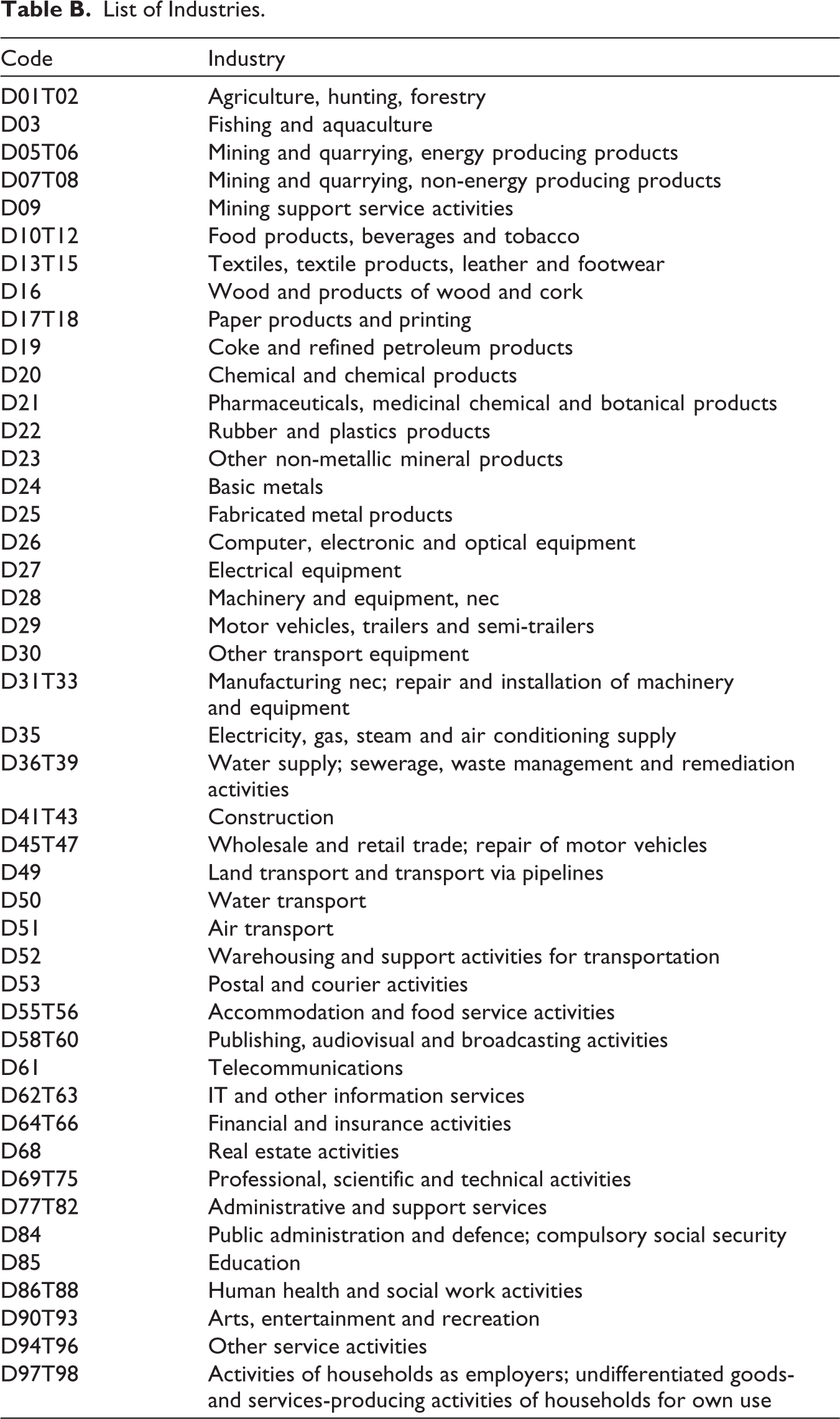
| Code | Industry |
| D01T02 | Agriculture, hunting, forestry |
| D03 | Fishing and aquaculture |
| D05T06 | Mining and quarrying, energy producing products |
| D07T08 | Mining and quarrying, non-energy producing products |
| D09 | Mining support service activities |
| D10T12 | Food products, beverages and tobacco |
| D13T15 | Textiles, textile products, leather and footwear |
| D16 | Wood and products of wood and cork |
| D17T18 | Paper products and printing |
| D19 | Coke and refined petroleum products |
| D20 | Chemical and chemical products |
| D21 | Pharmaceuticals, medicinal chemical and botanical products |
| D22 | Rubber and plastics products |
| D23 | Other non-metallic mineral products |
| D24 | Basic metals |
| D25 | Fabricated metal products |
| D26 | Computer, electronic and optical equipment |
| D27 | Electrical equipment |
| D28 | Machinery and equipment, nec |
| D29 | Motor vehicles, trailers and semi-trailers |
| D30 | Other transport equipment |
| D31T33 | Manufacturing nec; repair and installation of machinery and equipment |
| D35 | Electricity, gas, steam and air conditioning supply |
| D36T39 | Water supply; sewerage, waste management and remediation activities |
| D41T43 | Construction |
| D45T47 | Wholesale and retail trade; repair of motor vehicles |
| D49 | Land transport and transport via pipelines |
| D50 | Water transport |
| D51 | Air transport |
| D52 | Warehousing and support activities for transportation |
| D53 | Postal and courier activities |
| D55T56 | Accommodation and food service activities |
| D58T60 | Publishing, audiovisual and broadcasting activities |
| D61 | Telecommunications |
| D62T63 | IT and other information services |
| D64T66 | Financial and insurance activities |
| D68 | Real estate activities |
| D69T75 | Professional, scientific and technical activities |
| D77T82 | Administrative and support services |
| D84 | Public administration and defence; compulsory social security |
| D85 | Education |
| D86T88 | Human health and social work activities |
| D90T93 | Arts, entertainment and recreation |
| D94T96 | Other service activities |
| D97T98 | Activities of households as employers; undifferentiated goods- and services-producing activities of households for own use |