Investigating the Impact of Exchange Rate Volatility,Inflation and Economic Output on International Trade of India

Abstract

Four models have been constructed separately for exports of goods, imports of goods, exports of services and imports of services to explore the impact of exchange rate volatility, inflation and economic output on India’s foreign trade. AutoRegressive Distributed Lag (ARDL) bounds test run on monthly data over the period of 2011–2020 reports that in the long run, growth in production positively impacts the trade in goods and services. Rise in level of prices negatively impacts the exports of goods. In the short run, a rise in volatility brings a decline in the imports of goods but in the long run, it has a positive impact on the exports of goods. Volatile exchange rate has no impact on trade in services. An increase in inflation in the short run leads to a rise in the imports of goods but brings a decline in the trade of services.

Keywords

International trade exchange rate volatility India ARDL bounds goods and services

JEL Classification: F0, F1, F3, F4, F10, F14

I. Introduction

Boosting international trade is one of the primary concerns of the Government of every country and when it comes to a developing nation like India, the scope of it is much greater. India’s trade sectoral contribution in GDP has grown by approximately 60 per cent from 2000 to 2018. India’s share in world exports has increased from 0.6 per cent in 1991 to 1.7 per cent in 2018. The agenda of the current Government is to make India an emerging superpower by focusing on boosting exports and reducing dependence on imports. To achieve this target, rising current account deficit should definitely get some attention. In case of our economy, it should be noted that the balance of trade is negative because of the deficit in trade of goods, not services. In fact, the services sector is the key driver of India’s economic growth contributing more than 50 per cent of India’s Gross Value Added (at current price) for approximately last 20 years. Mounting contribution of services sector in the growth of the economy has led to the consideration of trade in services separately in this study. Hence, the need of the hour is to separately examine what factors currently affect the imports and exports of goods and services in order to handle them differently.

After the collapse of Bretton woods system in 1973, exchange rate volatility and trade linkages have been tested vastly. Even with the presence of enormous literature, the relationship between the two variables has been still a debatable question and therefore the relationship of trade with exchange rate volatility has been inconclusive over the years. The proposition of exchange rate volatility having negative effects on trade flows gained attention from Ethier’s model (Ethier, 1973) which is centred on a risk-averse firm, making a decision on imports in presence of uncertainty (volatility) in exchange rate movements. With the assumption of risk aversion, the trade response in the presence of exchange rate volatility is deductively negative, although the significance of this inverse relation diminishes with the speculative behaviour of the firm. Further, studies by Arize (1997), Clark (1973) and Doğanlar (2002) suggest that exchange rate volatility negatively impacts the international trade. On the contrary, the empirical literature has not always supported this theoretical argument (e.g., refer Baum & Çaglayan, 2010; Kroner & Lastrapes, 1993), which suggest a positive impact of volatility. Sercu (1992) showed that volatility could increase trade as it increases the probability that the price a trader receives might exceed trade costs. Sercu and Vanhulle (1992), on the other hand, theorise that rising volatility increases the value of exporting firms, thus, encouraging exports. De Grauwe (1988) argues that an increase in risk, in general, has both a substitution and an income effect that work in opposite directions (Goldstein & Khan, 1985). The substitution effect discourages risk-averse agents to export because it lowers the expected utility representing the attractiveness of the risky activity, while the income affects urges the risk-averse agents to increase their exports to avoid the possibility of a severe decline in the revenues. Taken together, these studies support the notion that even though firms are worse off with an increase in exchange rate risk, their response may be to export more rather than less.

Similarly, during the last decade, a mixed impact of exchange rate volatility has been observed on the foreign trade. Arize et al. (2008) shows that an increase in the volatility of the real effective exchange rate, exerts a significant negative effect upon export demand in both the short-run and the long-run in each of the eight Latin American countries considered for the study. Studies by Ekanayake et al. (2010) and Auboin and Ruta (2013) also suggest negative impact of exchange rate volatility on trade flows. Bahmani-Oskooee et al. (2016) observe no impact of exchange rate volatility on trade of Pakistan. According to Sharma and Pal (2018), exchange rate volatility has a dampening effect on exports of India. Bahmani-Oskooee and Gehlan (2018) studied the impact of exchange rate volatility, world income and real effective exchange rate on exports and imports of 12 African countries and the result indicates mixed impacts of volatility on exports and imports.

In response to this conflict in theoretical and empirical evidences, the main aim of our research is to investigate the interaction between real effective exchange rate volatility and international trade of India. Further, the inflation in the economy also deteriorates the trade balance of the economy (Stockman, 1985). Thus, it is important to consider the impact that inflation has on the trade in goods and services. Stockman (1981) showed that monetary policy expansion, exchange rate and country’s income impact the international trade. Pratikto (2012) suggests that the real effective exchange rate and inflation are important in explaining the movement of exports and imports of Indonesia. Mayer and Steingress (2020) study the effect of exchange rate changes on exports of 25 countries that are part of the Bank for International Settlements narrow effective exchange rate indexes and conclude that inflation and real exchange rate volatility has a positive impact on exports for most economies. Additionally, international trade of a country may be influenced by its production. Thus, production of goods and services is also considered for the study (Alshubiri et al., 2019).

Tharakan et al. (2005) showed that the determinants of exports of goods are different from that of software exports. Hence, in order to make India grow its share in the world trade, it is high time to understand that goods and services are two different commodities and they need different attention. For an economy like India, where services sector is the most dominant one, a study focusing on services separately from goods is lacking. So, a major contribution of the study will be the segregated analysis for goods and services. This will help policy makers to examine what factors should be considered relevant in case of goods and how those factors effect in case of services. Also, by taking post-recession data, the study depicts the current scenario prevailing in the economy. Additionally, various studies have either been inconclusive or found insignificant impact of volatility on international trade. This study has tried to establish a conclusive relationship between the two. Further research on this topic can explore the side of geopolitical dynamics on international trade. Additionally, foreign trade relations can be tested in a pre and post-COVID timeframe.

The paper is organised as follows. Section II covers materials and methods. Section III emphasises on results and discussions. Section IV provides conclusions and policy suggestions.

II. Materials and Methods

Estimation of Volatility

In order to estimate volatility, presence of volatility clustering and arch effect is checked in REER series. REER is considered as it takes into account the currencies of major trading partners of India and is adjusted for inflation. Since no arch effect is observed, REER_{% change} (or returns) are computed (Prakash, 2012) and then volatility is estimated using the annual rolling variances formula given below

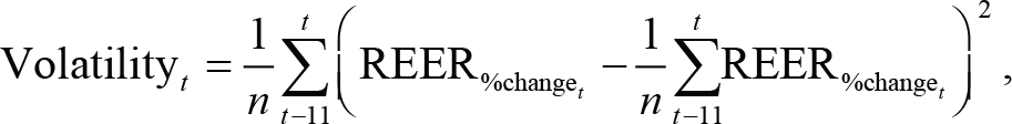
{Volatility}_{t} = \frac{1}{n} \sum_{t - 11}^{t} {({REER}_{{%change}_{t}} - \frac{1}{n} \sum_{t - 11}^{t} {REER}_{{%change}_{t}})}^{2},

where t ≥12 and n = 12.

For estimating volatility, data of REER from May 2010 to May 2020 is considered.

Expected Impact of the Variables Considered

Volatility of Real Effective Exchange Rate on Exports and Imports

Volatile exchange rates make international trade and investment decisions more difficult because volatility increases exchange rate risk. Exchange rate risk refers to the potential to lose money because of a change in the exchange rate (Suranovic, 2010). Thus, theoretically, a rise in volatility is expected to be negatively associated with the trade.

Inflation (Proxied by Consumer Price Index) on Exports and Imports

According to the theory, a rise in domestic inflation of a country makes its goods and services more expensive as compared to the imported products and hence, the demand for imported goods and services increases. Since a rise in domestic inflation decreases the competitiveness of the produced goods and services in the global market, exports decrease (Roldos, 1995).

Production (Proxied by Index of Industrial Production for Goods and Services_PMI¹ for Services) on Exports and Imports

Production of industrial goods and services of a country should be positively related with the exports of goods and services (considering the produced goods and services are exported) and negatively with the imports (considering the produced goods and services replace the imported products).

Model Estimation

According to the microeconomic theory, conventional demand functions are homogeneous degree zero in terms of price and income (Deaton & Muellbauer, 1980). Studies by Ekanayake et al. (2010), Gafar (1995), Matsubayashi and Hamori (2003) and Salas (1982) have taken income and prices as two important explanatory variables of demand. Therefore, international demand function should comprise a proxy of income of an economy or production in an economy for which GDP is the obvious choice as according to the circular flow of income, GDP = income = production = spending but its official estimates are typically only available on a quarterly basis, whereas index of industrial production (IIP) is a monthly statistic. Until now therefore, the Organisation for Economic Co-operation and Development (OECD) system of composite leading indicators has used the IIP as a reference series (for GDP), which is available on a monthly basis and has also historically at least, displayed strong co-movements with GDP (Fulop & Gyomai, 2012). Hence, the output produced by a nation has been proxied by IIP in case of goods and Services_PMI in case of services in the present study. A proxy of relative prices has to be taken, which we have proxied by consumer price index (Roldos, 1995). Since the present study in a way revolves around the international demand (imports of goods and services) and supply (exports of goods and services), exchange rate plays a crucial role and hence keeping in consideration, a vast literature on the impact of exchange rate volatility on foreign trade, exchange rate volatility is also taken as an independent variable in the model.

Stationarity of all series is ensured using augmented Dickey Fuller (ADF) test (Dickey & Fuller, 1979) and Zivot–Andrews test (Zivot & Andrews, 2002). Once the presence of structural breaks is established within the underlying variables, it cannot be ignored while estimating the cointegrating relationships. Therefore, taking into account the nature of the variables [that is a mix of I(1) and I(0)] and the presence of structural breaks, the study uses the ARDL bounds testing approach to cointegration for estimating the long-run relationship between trade and the factors impacting the trade—exchange rate volatility, inflation and production. Because ARDL itself does not take the issue of potential structural breaks into the system, a dummy variable is introduced in the model to represent the break point in the dependent variables. Given the small sized dataset, it is not feasible to define a dummy variable for each break because it would severely reduce the model’s degrees of freedom. Instead, we chose to include just one dummy variable for each model to account for disruption in the dependent variable (Stoian & Iorgulescu, 2020). Four models have been estimated which are presented below.

Impact of Volatility of REER, CPI and IIP on Exports of Goods

The estimated equation can be expressed as follows:

Log (Exports_Goods)_t = β₀ + β₁ Log(VOL)_t + β₂ Log(CPI)_t + β₃ Log(IIP)_t + β₄ Dummy_EXG + ε_t

The estimated ARDL representations of the model are given by the following:

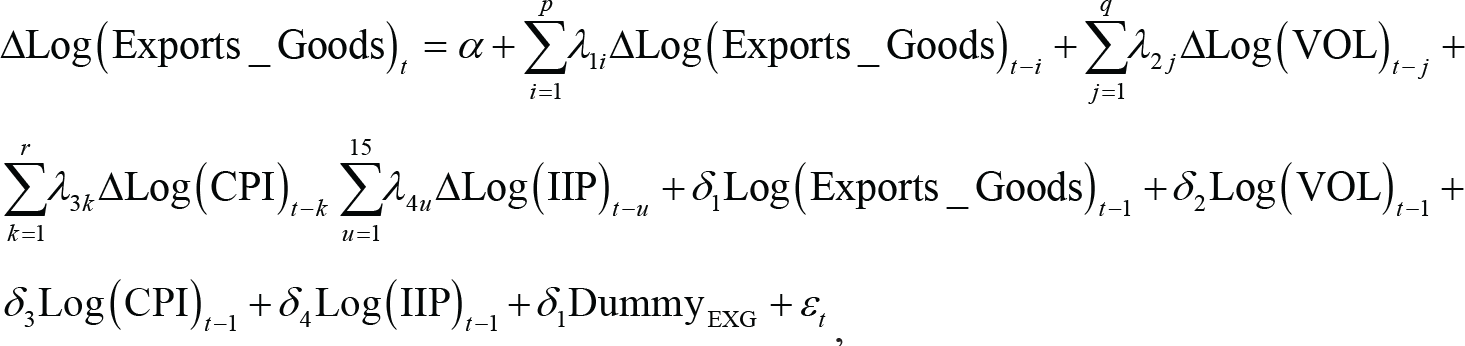
\begin{array}{l} Δ Log {(Imports_Goods)}_{t} = α + \sum_{i = 1}^{p} λ_{1 i} Δ Log {(Imports_Goods)}_{t - i} + \sum_{j = 1}^{q} λ_{2 j} Δ Log {(VOL)}_{t - j} + \\ \sum_{k = 1}^{r} λ_{3 k} Δ Log {(CPI)}_{t - k} \sum_{u = 1}^{15} Δ Log {(IIP)}_{t - u} + δ_{1} Log {(Imports_Goods)}_{t - 1} + δ_{2} Log {(VOL)}_{t - 1} + \\ δ_{3} Log {(CPI)}_{t - 1} + δ_{4} Log {(IIP)}_{t - 1} + δ_{1} {Dummy}_{IMG} + ε_{t} \end{array}

where Δ is the difference operator, Log(Exports_Goods) represents the log of exports of goods. VOL represents Volatility in REER, CPI represents inflation, IIP is the Industrial Production Index and ε is the error term. The Dummy_EXG represents the structural break of Exports of goods. It takes the value of 0 until January of 2015 and 1 thereafter.

The coefficients (λ1–λ5) represent the short-term dynamics of the model, whereas δ1–δ5 are the long-run coefficients. The values (p, q, r and m) are the selected number of lags of independent variables based on SIC. The bound testing has been performed to test for the existence of a long-run relationship among the variables by conducting an F-test for the joint significance of the coefficients of the lagged levels of the variables. The Wald coefficient restriction test has been performed to test the level effect with the null hypothesis of no level effect, that is:

H₀: δ1 = δ2 = … = δ5 = 0.

Impact of Volatility of REER, CPI and IIP on Imports of Goods

The estimated equation can be expressed as follows:

Log(Imports_Goods)_t = β₀ + β₁ Log(VOL)_t + β₂ Log(CPI)_t + β₃ Log(IIP)_t + β₄ Dummy_IMG + ε_t

The estimated ARDL representations of the model are given by the following:

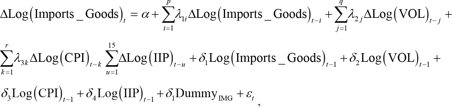
\begin{array}{l} Δ Log {(Exports_Goods)}_{t} = α + \sum_{i = 1}^{p} λ_{1 i} Δ Log {(Exports_Goods)}_{t - i} + \sum_{j = 1}^{q} λ_{2 j} Δ Log {(VOL)}_{t - j} + \\ \sum_{k = 1}^{r} λ_{3 k} Δ Log {(CPI)}_{t - k} \sum_{u = 1}^{15} λ_{4 u} Δ Log {(IIP)}_{t - u} + δ_{1} Log {(Exports_Goods)}_{t - 1} + δ_{2} Log {(VOL)}_{t - 1} + \\ δ_{3} Log {(CPI)}_{t - 1} + δ_{4} Log {(IIP)}_{t - 1} + δ_{1} {Dummy}_{EXG} + ε_{t} \end{array}

where Δ is the difference operator and Log(Imports_Goods) represents the log of imports of goods. The Dummy_IMG represents the structural break of Imports of goods. It takes the value of 0 before December of 2014 and 1 thereafter.

Impact of Volatility of REER, CPI and Services PMI on Exports of Services

The estimated equation can be expressed as follows:

Log(Exports_Services)_t = β₀ + β₁ Log(VOL)_t + β₂ Log(CPI)_t + β₃ Log(Services_PMI)_t + β₄ Dummy_EXS + ε_t.

The estimated ARDL representations of the model are given by the following:

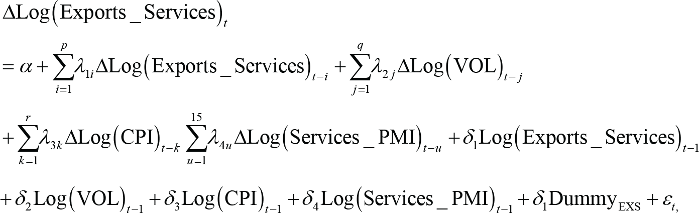
\begin{array}{l} \begin{array}{l} Δ Log {(Exports_Services)}_{t} \\ = α + \sum_{i = 1}^{p} λ_{1 i} Δ Log {(Exports_Services)}_{t - i} + \sum_{j = 1}^{q} λ_{2 j} Δ Log {(VOL)}_{t - j} \\ + \sum_{k = 1}^{r} λ_{3 k} Δ Log {(CPI)}_{t - k} \sum_{u = 1}^{15} λ_{4 u} Δ Log {(Services_PMI)}_{t - u} + δ_{1} Log {(Exports_Services)}_{t - 1} \end{array} \\ + δ_{2} Log {(VOL)}_{t - 1} + δ_{3} Log {(CPI)}_{t - 1} + δ_{4} Log {(Services_PMI)}_{t - 1} + δ_{1} {Dummy}_{EXS} + ε_{t,} \end{array}

where Δ is the difference operator and Log(Exports_Services) represents the log of exports of services. The Dummy_EXS represents the structural break of Exports of services. It takes the value of 0 before November 2017 and 1 thereafter.

Impact of Volatility of REER, CPI and Services PMI on Imports of Services

Initially, a log–log model was estimated for imports of services, as framed in previous cases but there was specification error in the model. Due to this, a log linear model is found suitable as Khan and Ross (1977) suggest that a log linear specification is better than a standard linear one on both empirical and theoretical grounds. That is, the former allows the dependent variable to react proportionally to an increase or decrease in the regressors and exhibits interaction between elasticities. Hence, a log-linear model has been framed for this case.

The estimated equation can be expressed as follows:

Log(Imports_Services)_t = β₀ + β₁ VOL_t + β₂ CPI_t + β₃ Services_PMI_t + β₄ Dummy_IMS + ε_t.

The estimated ARDL representations of the model are given by the following:

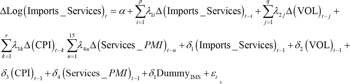
\begin{array}{l} Δ Log {(Imports_Services)}_{t} = α + \sum_{i = 1}^{p} λ_{1 i} Δ {(Imports_Services)}_{t - i} + \sum_{j = 1}^{q} λ_{2 j} Δ {(VOL)}_{t - j} + \\ \sum_{k = 1}^{r} λ_{3 k} Δ {(CPI)}_{t - k} \sum_{u = 1}^{15} λ_{4 u} Δ {(Services_P M I)}_{t - u} + δ_{1} {(Imports_Services)}_{t - 1} + δ_{2} {(VOL)}_{t - 1} + \\ δ_{3} {(CPI)}_{t - 1} + δ_{4} {(Services_P M I)}_{t - 1} + δ_{1} {Dummy}_{IMS} + ε_{t} \end{array}

where Δ is the difference operator and Log(Imports_Services) represents the log of imports of services. The Dummy_IMS represents the structural break of Imports of services. It takes the value of 0 before November 2017 and 1 thereafter.

The diagnostic tests consisting of the normality test, serial correlation test and heteroscedasticity test are run for each model. Finally, the stability of the long-run coefficients along with the short-run dynamics is evaluated by applying the CUSUM and CUSUMSQ (Brown et al., 1975). The CUSUM test uses the cumulative sum of recursive residuals, whereas the CUSUMSQ test is based on the cumulative sum of the squared recursive residuals.

Data

Month end values of all variables have been obtained from April 2011 to March 2020 for the study of goods. Data for services have been obtained from March 2012 to May 2020. Exports and imports of goods and IIP data have been obtained from IMF. Services trade data and real effective exchange rate series (starting from May 2010 to estimate volatility) have been obtained from RBI. Data of CPI have been obtained from OECD. Services_PMI data have been obtained from trading economics.

III. Results and Discussions

The ARDL bounds test can be applied to the series irrespective of whether they are I(0) or I(1) but this approach is not applicable if a series is integrated of order 2 or above. Thus, ADF test is applied and the results are presented in Table A1 in the appendix. It can be seen that none of the series is I(2). Lee and Chang (2005) argued that non-rejection of a unit root in a standard ADF test can be suspected when the sample under consideration contains structural breaks. The graphs of dependent variables also suggest the presence of structural breaks (Figures 1 –4 in the appendix). Thus, to address the issue, the unit root test developed by Zivot and Andrews (2002) which endogenously corrects for one structural break, is employed and the results are given in Table A2 in the appendix. All the series are stationary at level with a drift except Imports of Goods which is I(1). The break dates of all the series are also shown in the table. Since, the dataset comprises of a combination of I(0) and I(1) variables, ARDL bounds testing approach to cointegration is applied.

The structural break point for exports of goods is January 2015 and that for imports of goods is December 2014. The trade in goods had declined significantly after the structural break. Global commodity prices fell 38 per cent between June 2014 and February 2015 and the contraction in global demand and softening of crude and commodity prices had impacted the trade making imports go down after December 2014 significantly. On one side, the fall in crude oil prices reduced the bill of imports for India. On the other hand, domestic factors such as the non-availability of interest subvention coupled with high cost of credit had dissuaded small exporters to continue in exports. The uncertainty of policy front had also been a demotivating factor as exporters were unable to do their costing and take a call on future exports making exports go down significantly after January 2015.

The structural break point for exports and imports of services is November 2017. The trade in services had increased significantly after the structural break due to simplifications in GST processes. The earlier VAT/service tax regime in India was complicated due to multiple taxes, innumerable compliance obligations and tax cascading. The GST regime resulted in a simpler tax regime leading to a rise in both exports and imports of services. Further, export of information technology is an important source of foreign exchange, with India being the biggest exporter of IT services. Software exports have been zero-rated and input taxes paid are allowed as a refund. This perhaps brought the sudden increase specifically in the exports of services.

Model 1—Exports of Goods

Results of ARDL bounds test (see Table A3 in the appendix) show that the overall model is significant (F-statistic −12.96). The change in exports of goods is related to itself with a lag of 2 months, to volatility of exchange rates and CPI with a lag of a year, to IIP with a lag of 11 months. Long-run coefficients show that in the long term, 1 per cent rise in CPI brings a decline of 0.17 per cent in exports of goods. This negative relationship is consistent with our expectations. As prices go up, exports become expensive in the global market and hence decline. As production goes up by 1 per cent, exports of goods significantly move up by 1.28 per cent. This positive relationship is also in line with our expectations. Production impacts the exports of goods positively and production of goods domestically is important to lift exports in the long run. A percentage rise in volatility of exchange rate significantly and positively impacts the exports of goods by 0.12 per cent. Significance of structural break dummy suggests that exports have declined after January 2015 (for results, refer Table A4 in the appendix).

Since the coefficient of error correction term is negative and significant (see Table A6 in the appendix), short-term error correction mechanism is working in the model suggesting that percentage change in volatility of exchange rate with lag 8 positively impacts the percentage change in exports of goods, whereas with lag 11, it negatively impacts the percentage change in exports of goods. Change in IIP impacts the change in exports of goods positively at level, with lags 2, 8 and 9 and negatively with lag 10. Percentage change in CPI negatively impacts the percentage change in exports of goods with lag 6 and positively with lag 2. The short-term results indicate that volatility of exchange rate and inflation has a mixed impact on exports of goods unlike the clear long-term results. Structural break negatively impacts the change in exports in the short term.

Model 2—Imports of Goods

Results of ARDL bounds test (see Table A3 in the appendix) show that the overall model is significant (F-statistic −17.96). The change in imports of goods is related to itself, volatility of exchange rates with a lag of 2 months, to IIP with a lag of a year, to CPI with a lag of 3 months. Long-run coefficients show that in the long term, 1 per cent rise in IIP increases the imports of goods by 1.7 per cent (for results, refer Table A4 in the appendix). This positive relationship is inconsistent with our expectations. As production rises, imports should go down, but this result indicates two possibilities; one is that India is importing raw material to support the rise in production or the other is that India does not produce what it imports. Additionally, the coefficients of CPI and volatility of exchange rates are not significant in the long run suggesting goods that the country imports are so essential that even if prices and volatility change, imports do not get impacted. Crude oil and gold are the biggest imports of India; the country does not produce both the products, imports it and further processes it and hence such a relationship is justified. The significance of structural break dummy suggests that imports have declined after December 2014.

Since the coefficient of error correction term is negative and significant (see Table A7 in the appendix), short-term error correction mechanism is working in the model suggesting that percentage change in volatility of exchange rate with lag 1 negatively impacts the percentage change in imports of goods. Percentage change in CPI impacts the change in imports of goods positively with a lag of 2 months implying that rising inflation makes the domestic goods expensive, and therefore, the demand for imported goods rise in the short term. Structural break negatively impacts the change in imports in the short term; however, the impact is not significant.

Model 3—Exports of Services

Results of ARDL bounds test (see Table A3 in the appendix) show that the overall model is significant (F-statistic −18.47). The change in exports of services is related to itself with a lag of a year, volatility of exchange rates at level, IIP at level, CPI with lag of 6 months. Long-run coefficients show that in the long term, 1 per cent rise in Services_PMI increases the exports of services by 0.08 per cent (For results, refer Table A5 in the appendix). This positive relationship is consistent with the expectations. As production of services rises, exports of services should go up. The coefficients of CPI and volatility of exchange rates are not significant in the long run suggesting that services that the country exports are so in demand that even if prices and volatility change, exports of services do not get impacted. India is the biggest exporter of IT services in the world and hence such results are very much convincing. Significance of structural break dummy suggests that exports have increased after November 2017.

Since the coefficient of error correction term is negative and significant (see Table A8 in the appendix), short-term error correction mechanism is working in the model suggesting that change in Services_PMI positively impacts the change in exports of services at level and a percentage change in CPI with lag 5 negatively impacts the change in exports of services. Structural break positively impacts the change in exports of services in the short run.

Model 4—Imports of Services

Results of ARDL bounds test (see Table A3 in the appendix) show that the overall model is significant (F-statistic −17.48). The change in imports of services is related to itself with a lag of a year, to volatility of exchange rates and IIP at level and to CPI with a lag of 10 months. Long-run coefficients show that in the long term (For results, refer Table A5 in the appendix), the coefficients of exchange rate volatility and CPI are not significant in the long run indicating that change in volatility and inflation do not impact the imports of services by Indians. India perhaps does not produce those services that are imported and hence Indians will keep on importing them even if they become expensive or the exchange rate becomes volatile. A unit change in production of services will increase the imports of services by 0.01 per cent, showing that perhaps services that are being produced require imports of some inputs. Significance of structural break dummy suggests that imports of services have increased after November 2017.

Since the coefficient of error correction term is negative and significant (see Table A9 in the appendix), short-term error correction mechanism is working in the model suggesting that a unit change in CPI at level negatively impacts the change in imports of services and positively with lag 9. Change in Services_PMI positively impacts the change in imports of services at level. Structural break positively and significantly impacts the change in imports of services in the short run.

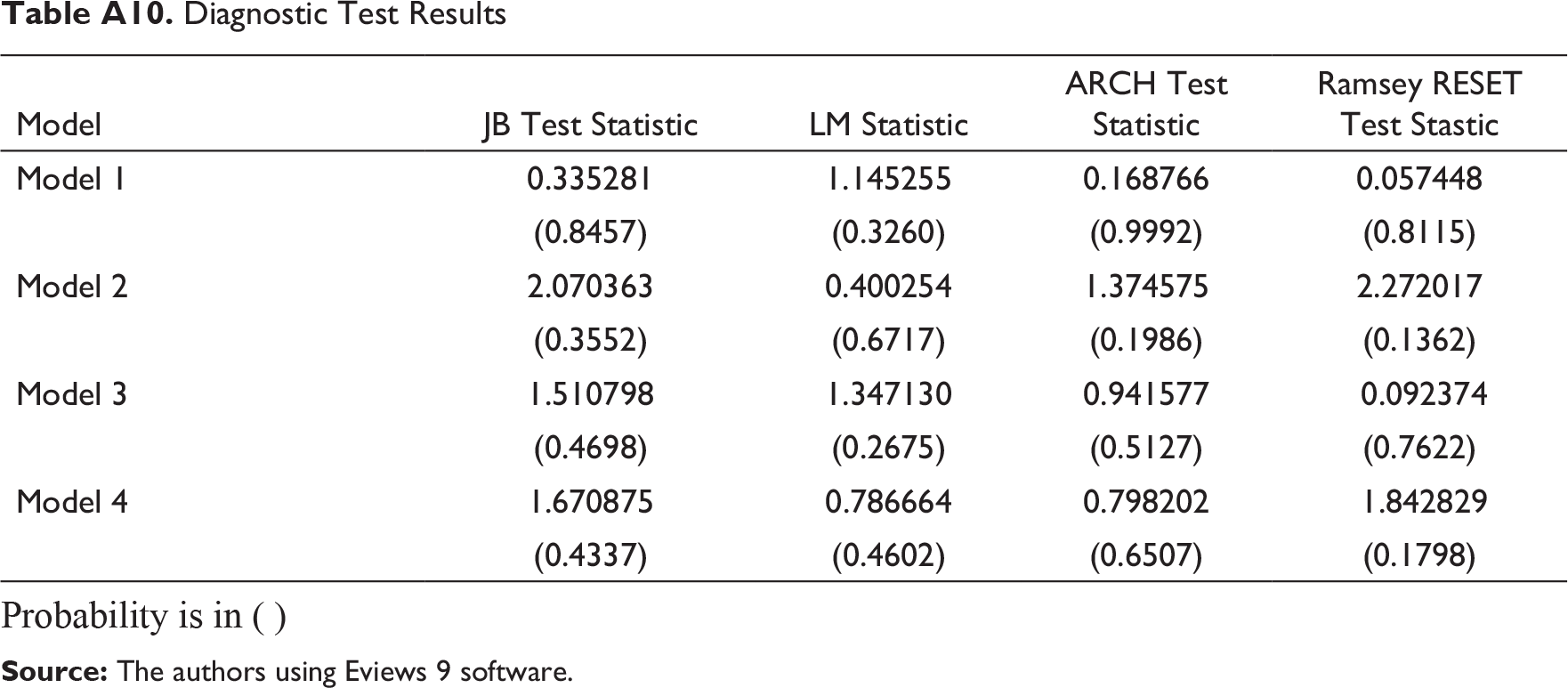
All required diagnostic tests are run on every model (see Table A10 and Figures 5 –8 in the appendix for results). Histogram for testing normality, Breusch–Godfrey LM test to detect serial correlation in the model, and ARCH test is run to check for heteroskedasticity. Also, for stability, CUSUMSQ and CUSUM are observed for each model. Ramsey test is run for model specification. There is no model specification error observed in any model.

IV. Conclusion and Policy Suggestions

In the long run, exports of goods are significantly and positively impacted by the production and negatively by inflation. Hence, producing goods domestically and monitoring the prices of the goods exported are two crucial aspects to consider while thinking of boosting exports of goods. Additionally, negative impact of volatility in exchange rates is not observed in case of exports of goods. Rather, the volatility has a significant positive impact on exports of goods. The result is consistent with the studies by Sercu and Vanhulle (1992) and De Grawe (1988). Further, imports of goods are positively and significantly related to the production, indicating two possibilities; one is that India is importing raw material to support the rise in production or the other is that India does not produce what it imports. Since inflation and volatility also do not significantly impact the imports of goods, the possibility of latter state to prevail is more. Crude oil and gold are the biggest imports of India; the country does not produce both the products, import it and further processes it and hence such a relationship is justified. Moreover, crude oil is the essential commodity, which is imported the most, therefore inflation and volatility not impacting such imports is justified. In the long run, exports of services are positively and significantly impacted by Services_PMI, not by inflation, and volatility indicating that the services that India exports the most that are IT, telecommunication services are so in demand that a change in inflation and volatility is not able to impact the demand. Further, imports of services are positively impacted by the production of services implying what India produces require inputs that need to be imported. The volatility in exchange rate, and inflation do not significantly impact the imports of services. India imports travelling services the most and hence according to the results, a volatile exchange rate or a rise in inflation will also not dampen the demand of travelling by Indians.

In order to make India an emerging superpower, positive trade balance is very crucial and hence the ‘Make in India’ initiative is good for the economy. Higher production of goods and services will boost exports of both goods and services, sustaining our current account deficit. Hence, the Government should further focus on accelerating the pace of this initiative. Our economy has been an inflation targeting economy and hence that focus should be maintained in order to avoid dampening effect of inflation on the exports of goods. No relationship has been found between exports of services and CPI in the long run, implying that a rise in price of such services would not dampen their exports. Hence, the demand of services would still be there, and this should be utilised to further boost the revenues from the services sector. In the long term, the negative impact of volatility has not been discovered in any of the models. Therefore, the volatility in exchange rates may not be a prime concern for the policymakers in India.

Footnotes

Acknowledgement

The authors are grateful to Professor C. P. Gupta, who gave us his valuable suggestions to improve the content of this study. The authors also acknowledge the help received from their senior, Prateek Bedi. Undoubtedly, the editorial board of the Indian Economic Journal has contributed enormously in this script by suggesting some very important revisions. The paper would have been impossible without the patience and the efforts shown by the editorial board.

Declaration of Conflicting Interests

The authors declared no potential conflicts of interest with respect to the research, authorship and/or publication of this article.

Funding

The authors received no financial support for the research, authorship and/or publication of this article.

Notes

Appendices

Table A10. Diagnostic Test Results

Model	JB Test Statistic	LM Statistic	ARCH Test Statistic	Ramsey RESET Test Stastic
Model 1	0.335281	1.145255	0.168766	0.057448
	(0.8457)	(0.3260)	(0.9992)	(0.8115)
Model 2	2.070363	0.400254	1.374575	2.272017
	(0.3552)	(0.6717)	(0.1986)	(0.1362)
Model 3	1.510798	1.347130	0.941577	0.092374
	(0.4698)	(0.2675)	(0.5127)	(0.7622)
Model 4	1.670875	0.786664	0.798202	1.842829
	(0.4337)	(0.4602)	(0.6507)	(0.1798)

Source: The authors using Eviews 9 software.

Probability is in ( )

References

Alshubiri

Elheddad

Doytch

(2019). The impact of fish production on marine trade balance and foreign direct investment: An empirical study of the GCC economies. Marine Policy , 116, 103660.

Arize

A. C.

(1997). Conditional exchange-rate volatility and the volume of foreign trade: Evidence from seven industrialized countries. Southern Economic Journal , 64, 235–254.

Arize

A. C.

Osang

Slottje

D. J.

(2008). Exchange-rate volatility in Latin America and its impact on foreign trade. International Review of Economics & Finance , 17(1), 33–44.

Auboin

Ruta

(2013). The relationship between exchange rates and international trade: A literature review. World Trade Review , 12, 577–605.

Bahmani-Oskooee

Iqbal

Salam

(2016). Short run and long run effects of exchange rate volatility on commodity trade between Pakistan and Japan. Economic Analysis and Policy , 52, 131–142.

Bahmani-Oskooee

Gelan

(2018). Exchange-rate volatility and international trade performance: Evidence from 12 African countries. Economic Analysis and Policy , 58, 14–21.

Baum

C. F.

Caglayan

(2010). On the sensitivity of the volume and volatility of bilateral trade flows to exchange rate uncertainty. Journal of International Money and Finance , 29(1), 79–93.

Brown

Durbin

Evans

(1975). Techniques for testing the constancy of regression relationships over time. Journal of the Royal Statistical Society. Series B (Methodological) , 37(2), 149–192. Retrieved May 23, 2020, from www.jstor.org/stable/2984889

Clark

P. B.

(1973). Uncertainty, exchange risk, and the level of international trade. Economic Inquiry , 11(3), 302–313.

10.

De Grauwe

(1988). Exchange rate variability and the slowdown in growth of international trade. IMF Economic Review , 35, 63–84.

11.

Deaton

Muellbauer

(1980). Economics and consumer behavior . Cambridge University Press.

12.

Dickey

D. A.

Fuller

W. A.

(1979). Distribution of the estimators for autoregressive time series with a unit root. Journal of the American Statistical Association , 74(366a), 427–431.

13.

Doğanlar

(2002). Estimating the impact of exchange rate volatility on exports: Evidence from Asian countries. Applied Economics Letters , 9(13), 859–863.

14.

Ekanayake

E. M.

Ledgerwood

J. R.

D’Souza

(2010). The real exchange rate volatility and US exports: An empirical investigation. International Journal of Business and Finance Research , 4(1), 23.

15.

Ethier

(1973). International trade and the forward exchange market. The American Economic Review , 63, 494–503.

16.

Gafar

(1995). Some estimates of the price and income elasticities of import demand for three Caribbean countries. Applied Economics , 27(11), 1045–1048.

17.

Goldstein

Khan

(1985). Income and price elasticities in foreign trade. In Jones

Kenen

(Eds.), Handbook of international economics (pp. 1041–1105). Amsterdam.

18.

Fulop

Gyomai

(2012). Transition of the OECD CLI system to a GDP-based business cycle target. Retrieved from http://www.oecd.org/std/leading-indicators/49985449.pdf

19.

Khan

M. S.

Knud Z.

(1977). The functional form of the aggregate import demand equation. Journal of International Economics , 7, 149–160.

20.

Kroner

K. F.

Lastrapes

W. D.

(1993). The impact of exchange rate volatility on international trade: reduced form estimates using the GARCH-in-mean model. Journal of International Money and Finance , 12(3), 298–318.

21.

Lee

C.-C.

Chang

C.-P.

(2005). Structural breaks, energy consumption, and economic growth revisited: evidence from Taiwan. Energy Economics , 27, 857–872.

22.

Matsubayashi

Hamori

(2003). Some international evidence on the stability of aggregate import demand function. Applied Economics , 35(13), 1497–1504.

23.

Mayer

Steingress

(2020). Estimating the effect of exchange rate changes on total exports. Journal of International Money and Finance , 106, 102184.

24.

Prakash

(2012). Major episodes of volatility in the Indian foreign exchange market in the last two decades (1993–2013): Central Bank’s Response. RBI Occasional Papers , 33(1–2), 162–199.

25.

Pratikto

(2012). Dynamics of Indonesia’s international trade a VAR approach. Procedia Economics and Finance , 4, 149–159.

26.

Roldos

J. E.

(1995). Supply-side effects of disinflation programs. Staff Papers—International Monetary Fund , 42(1), 158. doi:10.2307/386734.

27.

Salas

(1982). Estimation of the structure and elasticities of Mexican imports in the period 1961–1979. Journal of Development Economics , 10(3), 297–311.

28.

Sercu

(1992). Exchange rates, volatility and the option to trade. Journal of International Money and Finance , 11(6), 579–593.

29.

Sercu

Vanhulle

(1992). Exchange rate volatility, international trade, and the value of exporting firms. Journal of Banking & Finance , 16(1), 155–182.

30.

Sharma

Pal

(2018). Exchange rate volatility and India’s cross-border trade: A pooled mean group and nonlinear cointegration approach. Economic Modelling , 74, 230–246.

31.

Stockman

A. C.

(1981). Effects of inflation on the pattern of international trade (NBER Working Paper No. 0713). National Bureau of Economic Research.

32.

Stockman

A. C.

(1985). Effects of inflation on the pattern of international trade. Canadian Journal of Economics , 18, 587–601.

33.

Stoian

Iorgulescu

(2020). Fiscal policy and stock market efficiency: An ARDL bounds testing approach. Economic Modelling , 90, 406–416.

34.

Suranovic

S. M.

(2010). Exchange rate volatility and risk. In Suranovic

S. M.

(Ed.). International Finance Theory and Policy (pp. 448–452). Saylor Foundation.

35.

Tharakan

P. K. M.

Beveren

I. V.

Ourti

T. V.

(2005). Determinants of India’s software exports and goods exports. Review of Economic Studies , 87(4), 776–780.

36.

Zivot

Andrews

D. W. K.

(2002). Further evidence on the great crash, the oil-price shock, and the unit-root hypothesis. Journal of Business & Economic Statistics , 20(1), 25–44.