
Abstract
While the basic exchange rate regime has stayed the same since the liberalising reforms of the 90s, its implementation has varied over the years. The article assesses the evolution of India’s nominal exchange rate regime and its suitability under inflation targeting. It also examines the evolving impact on trade, inflation, currency and financial markets, country risk premium and the cost of borrowing. The analysis suggests a flexible exchange rate with intervention to prevent excess volatility as well as misalignment from competitive real exchange rates, while allowing some volatility to aid price discovery in foreign exchange markets, would work best in inflation targeting emerging markets.
Introduction
The Reserve Bank of India’s (RBI) description of the Indian exchange rate regime is unchanged since the liberalisation of the 1990s. It is said to be market-determined, with intervention only to prevent excess volatility. But the range of movement shows considerable variation over the past 30+ years.
The basic policy was therefore implemented very differently with varying outcomes. The article explores these variations and in particular if and how the regime changed after inflation targeting was implemented in 2013. For purists, inflation targeting demands a perfect float. But all emerging market (EM) central banks (CBs) hold reserves and intervene.
Canonical inflation targeting wants exchange rates to float as the correct response to capital flows. Policy should respond to exchange rate fluctuations only after they affect inflation or output, implying domestic interest rates need not immediately rise. Interest rate defence of the exchange rate is not required in advanced economies (AEs) since overshooting of nominal exchange rate tends to reverse. An expected appreciation towards equilibrium levels allows interest rates to remain low. In EMs, however, overshooting tends to intensify and become persistent as it provokes capital flight. But raising interest rates sharply can aggravate this as growth falls and country risk rises. Thin markets can get trapped in cumulative one-way movements and panics. As self-fulfilling depreciation raises inflation, policy rates have to rise eventually.
Contrary to conventional macroeconomic theory, therefore, merely relying on the flexibility of exchange rates is not enough to shield the domestic economy from global spillovers. Pragmatic policymakers understand this. Most EM CBs intervene in foreign exchange (FX) markets and use prudential regulation in order to reduce nominal volatility. 1 FX reserves serve an essential precautionary purpose, enabling intervention as well as reducing country risk perceptions. Two instruments for two targets work better than trying to do everything through the interest rate. We assess the compatibility of India’s exchange rate regime with inflation targeting.
An exchange rate regime affects aggregate demand (exports), market volatility and inflation (Corden, 2002). In addition, we evaluate how these effects varied over the years. This assessment of outcomes allows derivation of best practices in the Indian context.
Export growth rose sharply in 2021–2022, despite the pandemic, before slowing with global growth. The real effective exchange rate (REER) was maintained around competitive levels over this period, unlike the sustained real appreciation after 2014. But measures to reduce export bottlenecks were also responsible for the strong performance. Intervention helped the rupee approach equilibrium in an orderly way despite large capital flow movements and USD fluctuations. Deeper FX markets have raised daily volatility but intervention needs to avoid reducing it too much.
While better anchoring of inflation expectations and falling oil intensity of production helped reduce pass through of commodity price rise, the new tendency for the USD to strengthen with international oil prices implies intervention to reduce rupee depreciation in such periods could abort inflationary impulses from international commodity price shocks. Two-way movement of the rupee would encourage hedging.
As RBI Governor during the early reform years, Dr Rangarajan set in place the basic policy that has worked well through the turbulent years that followed despite much learning and fine-tuning as the economy plunged into new waters. It is appropriate, therefore, that a paper for a special issue dedicated to his work explores this process. Many of the topics taken up were already flagged in Rangarajan and Prasad (2008): Volatility in excess of macroeconomic fundamentals due to capital inflows can inhibit international trade; help from nominal appreciation in the management of inflation; the importance of two-way movements in introducing an element of uncertainty in the market and reducing speculative one-way positions; the sensitivity of inflows and their persistence to global developments, creating uncertainty for policymakers; intervening to depreciate the currency can cause real exchange rate appreciation through inflation, which is less desirable than nominal exchange rate appreciation; the benefits of a ‘middle way’ between fixed and free-floating exchange rates in reducing volatility yet preventing real misalignment without painful domestic deflation or inflation; using a judicious mix of multiple instruments.
The structure of the article is as follows: Section II presents stylised facts on India’s exchange rate fluctuations and market perceptions; Section III discusses how India’s exchange rate regime interacted with inflation targeting; Section IV analyses the effect of the exchange rate on ‘Aggregate Demand’ in the first subsection, ‘Excess Volatility and Risk Premium’ in the second subsection, and ‘Inflation’ in the third. Section V concludes with policy implications.
Facts and Perceptions
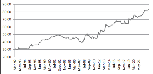
Figure 1 shows the behaviour of the nominal exchange rate differed in each of the three post-liberalisation decades. After trend nominal depreciation in the first decade, two-way movement began with appreciation in 2001 that continued until the sharp depreciation in 2008. Volatility rose after the global financial crisis (GFC). There was substantial two-way movement with some appreciation following episodes of sharp depreciation. Markets tend to get excited when there is volatility after a period of stability or a reversal in a sustained past direction. There are newspaper headlines when the rupee breaches a new low even if it is only a marginal change.
Average Monthly INR/USD.
Average Monthly INR/USD.
The 2010s was a decade of large global liquidity due to quantitative easing (QE) in AEs. Risk-on inflows to EMs in a search for yields became risk-off outflows during global shocks. Even so, outflows tended to reverse quickly, creating large movements in nominal exchange rates (Figure 1). It was also a decade of high inflation and large fiscal and current account deficits (CADs).
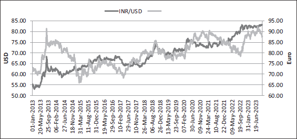
Comparatively, the period 2014–2017 was one of relative calm. This is clearer in Figure 2, with daily data. Table 1 shows year-on-year changes to be low over 2014–2017 compared to the large fluctuations after the GFC period. In 2017 there was even an overall nominal appreciation.
Daily Exchange Rate of Rupee versus USD and Euro.
Nominal End December Exchange Rate: Depreciation (+) or Appreciation (−).
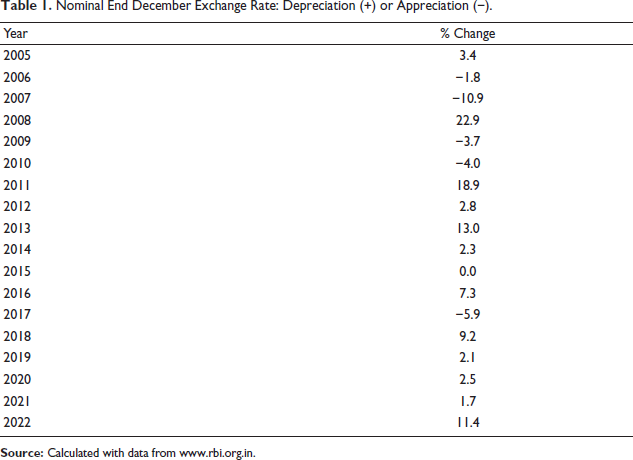
Table 2 calculates the yearly volatility as the percentage change between the highest and the lowest monthly exchange rate within a year and its standard deviation. External shocks such as the East Asian crisis (1995–1998), the GFC, the Euro-debt crisis of 2011, the Fed taper-on of 2013 and Fed moves to normalise monetary policy in 2018 are associated with higher volatility, due to risk-on risk-off shifts in foreign capital and changes in the dollar value, not to discovery of fundamental value in domestic markets.
Yearly Volatility of the Exchange Rate.
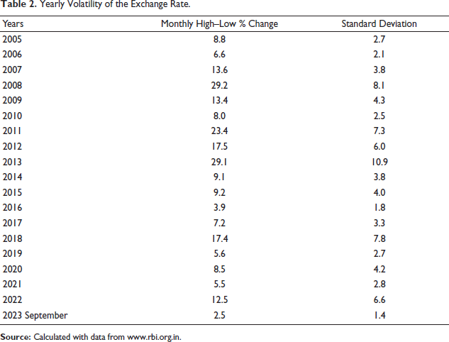
Despite the continuing policy to reduce excess volatility, in the GFC period, intervention became minimal because of the fear that inflows were now too large. Volatility rose, forcing heavy intervention that was able to substantially reduce volatility after the taper tantrum in 2013 (Goyal, 2018). But real appreciation above equilibrium, despite a large CAD and higher relative inflation, increased the chances of a sharp depreciation, which occurred in 2018. After that more even two-way nominal movement with middling volatility (Table 2) delivered stability around competitive equilibrium exchange rates. Thus, intervention is effective but neither too much nor too little is appropriate. It should not result in persistent misalignment.
There were large stretches of time with low volatility. The yearly standard deviation was just 2.5 even during the calm after the GFC and only 1.8 even in 2016 and 1.4 in 2023. Daily exchange rate volatility (Figure 2) did, however, increase from very low levels in the relatively fixed exchange rate regime immediately after the 90s reforms, in line with a steady deepening of domestic FX markets. 2 Figure 2 shows volatility to be higher in the INR/Euro pair since intervention is mostly in USD.
Indian experience shows it is possible to reduce excess depreciation despite global risk-on and offs. While in most EMs exchange rate volatility rose after the taper-tantrum in 2013, in India, it actually fell.
How did the adoption of inflation targeting affect the exchange rate regime?
Inflation targeting began informally in 2014 although the formal agreements were completed by 2016. The mandate of the Monetary Policy Committee (MPC) is ‘to primarily achieve price stability while keeping in mind the objective of growth’, with the repo rate as the instrument. The exchange rate continued to be the responsibility of the RBI, and there was no change in the exchange rate regime. The figures and tables above do not show any break in outcomes. Volatility varied with external shock-related capital flows and the degree of intervention. But the nominal rate was set in active FX markets.
Neither systemic factors nor past variables should affect nominal rates in efficient markets that immediately factor in news. Research finds random walk to outperform all fundamental-based short-term forecasts in a full float. Market participants, however, still make short-term forecasts based on news and on spotting trends and patterns.
As the price of money, the fundamental determinants of the nominal exchange rate are relative money supplies, prices, output and interest rates. Also, factors affect the demand and supply of FX now and in the future. Although in the short term, market perceptions and policy can affect the exchange rate, long-term departures from equilibrium levels cannot be sustained. Over the longer term, macroeconomic fundamentals including relative productivity and real wages determine the real equilibrium rate. But uncertainty surrounds this equilibrium level, especially in an economy undergoing structural transformation. The CB has a role in preventing persistent REER deviations.
Market-friendly controls have gained more acceptability after the GFC and the excessive capital movements that followed. Much research, including from the International Monetary Fund (IMF), argues for the use of prudential capital flow management (CFM) techniques. FX reserves reduce risks and crises in EMs. Intervention, including CFM, is consistent with international laws and conventions. It is desirable if it corrects market overshooting, but harmful if it sustains deviations from equilibrium values. Moreover, the FX market is not a typical market. Market players are not equal since the CB has more information and ammunition than any other market participant. Its policy with respect to the exchange rate, including intervention and communication, can affect outcomes. RBI has access to all these techniques.
Fearing FX markets were now too large, RBI stopped intervening after the GFC, despite large outflows. But, as depreciation rose sharply, it restricted FX markets, which only encouraged one-way positions to migrate abroad, where they are not regulated. There is evidence the non-deliverable forward market grew 3 over 2010–2013 when restrictions were imposed. Market freedoms were gradually restored after 2014, but the realisation that policy could be effective led to the exchange rate being tightly managed over 2014–2015. Intervention thus veered from too little after the GFC to too much after 2014.
India’s sequenced approach to capital account convertibility gives scope for intervention. For example, debt inflows are only allowed as a percentage of domestic market size. Capital flows are welcome but along with the domestic market deepening so diversity increases but volatility is contained. This approach saved India from the large interest rate volatility that Indonesia experienced during the taper tantrum.
While surges and sudden stops in capital flows make intervention necessary, it must not be one-sided and has to be strategic, based on domestic market structure and in line with fundamentals. Timing must use market intelligence on net open positions, order flow, bid-ask spreads (when one-sided positions dominate dealers withdraw from supplying liquidity and spreads rise), turnover and share of interbank trades.
For example, at the end of August 2013, one of the most effective rupee-stabilising measures was the FX swap window announced for oil marketing companies, since it took a large chunk of dollar demand out of the market. Capital flows do not always match the net import gap, so RBI has a role in closing any short-term demand–supply mismatch. RBI gains from selling dollars when the rupee has fallen (as long as it does not fall further) and buying dollars when the rupee has risen. So it is best to enter markets after some exchange rate overshooting in order to impose loss on outflows.
The large stock of reserves ensures market interventions command respect. But accumulating reserves is easier than losing them. However, large reserves are markets tend to get worried if they are falling. There are costs of holding large reserves and of too much intervention. The CB ends up supporting the USA and not its own government borrowing and it sacrifices interest income. But holding reserves and then not using them when required is the most costly!
Typically, there is less information and more uncertainty in EMs, so signalling can be quite effective. Signals that the RBI was unable to intervene and the INR should be left to the markets had a large but counter-productive impact in 2011, while reassurance calmed markets in 2013 and in the post-pandemic period. Overshooting from fundamental currency values and one-way feedback trading hurts markets also. Since markets are much larger now, the RBI can influence market expectations but cannot act totally against them. There are a variety of signals. Interventions themselves convey a strong signal, even without committing to a specific target exchange rate or deviating from the announced position of intervening only to prevent excess volatility. The central value need not be announced and can change with inflation differentials in order to prevent real over- or under-valuation.
With all these measures available, the interest rate defence is not necessary to prevent overshooting. Interest rates were raised during the taper tantrum and in 2018. They could not prevent outflows but triggered a slowdown. In the post-pandemic period policy successfully used multiple instruments to reduce exchange rate volatility, while aligning the repo rate to the needs of the domestic cycle.
There is an argument that less intervention and more rupee depreciation would improve the CAD. But less intervention led to a chaotic fall and jittery markets in 2011. If inflation rises with nominal depreciation, real appreciation results, defeating the policy since it is real appreciation that affects trade. It is best therefore for policy to prevent over-depreciation due to global risks. Inflation-targeting purists forget that it is dangerous to apply textbook economic theory based on perfect markets regardless of the time and the place.
The use of multiple instruments can mitigate over-reliance on intervention. Much research and recent experience suggest that all available instruments should be used to moderate volatility in nominal variables. This would prevent excess deviations of real variables, such as real interest and exchange rates, from equilibrium levels. These affect, and deviations can distort, real sector decisions. In the previous decade when Indian growth and investment rates fell, real interest rates ranged from −10 to +6 per cent. While depreciation does benefit some exporters, all are hurt by the excess volatility of exchange rates.
In the sections to follow, we examine successively how the exchange rate regime affected, first, net exports and aggregate demand, second, financial stability and, third, imported costs and inflation.
Effects of the Exchange Rate
Aggregate Demand
The exporter gains from real rupee depreciation but at the cost of the importer and the consumer. Small firms are the largest exporters and source of employment. They operate on thin margins, however, and value help from a cheap rupee. But only firms with large value added (such as textiles and agriculture) gain substantially from depreciation. Firms with high import dependence see their costs rise. Those with foreign currency debt also lose from depreciation.
The REER, which corrects for relative inflation, gives weights to bilateral real exchange rates according to major trading partners. The way it is calculated, a rise in the nominal effective exchange rate (NEER) or the REER is an appreciation, and vice versa. A relative constancy of the real exchange rate around the REER established after the double devaluation in the early 90s liberalisation had been a feature of post-reform policy. In 2004–2005, when the index base was changed, its level was almost the same as it was the early 90s—this was regarded as the competitive or fair-valued exchange rate since export growth had been good with the REER at this level. As depreciation corrected for India’s higher inflation, it was at this level even in 2006.
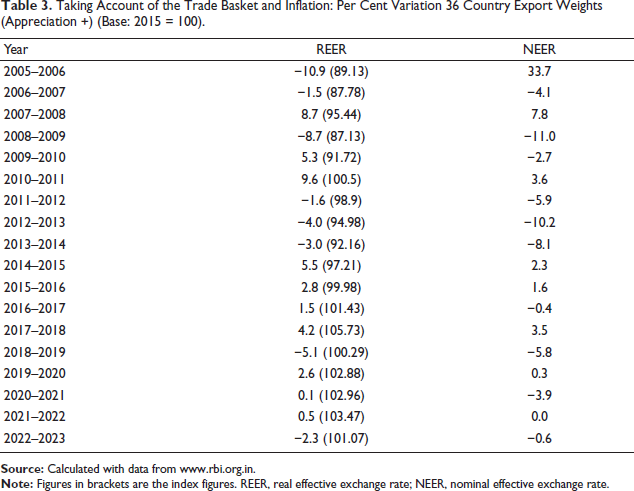
Table 3 shows two-way movements in REER in the first 10 years driven by external crises-related fluctuations in foreign capital flows. India’s large trade deficit ruled out sustained appreciation as a means of absorbing foreign inflows. But there was sustained real appreciation from 2014. When 2015 was taken as the new base, it was above 110 in the old 2004–2005 base. Appreciation continued and it reached 106 in 2017–2018. Export growth slowed in 2012 and remained low until mid-2018, despite a recovery in world growth.
Taking Account of the Trade Basket and Inflation: Per Cent Variation 36 Country Export Weights (Appreciation +) (Base: 2015 = 100).
Taking Account of the Trade Basket and Inflation: Per Cent Variation 36 Country Export Weights (Appreciation +) (Base: 2015 = 100).
But what is the equilibrium or fair value of the REER? Other factors, apart from relative inflation, affect equilibrium real exchange rates. The REER gives the Indian basket that can be purchased by a foreign basket. A rise in the relative supply of Indian products, perhaps due to a rise in productivity, would require a real depreciation of the rupee. But in an EM, the purchasing power parity exchange rate exceeds unity because real wages and the price level are relatively lower. As wages and non-traded goods prices rise with development, there is a real appreciation. This is the Balassa–Samuelson effect.
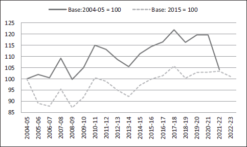
Because of many causal factors, the precise value of the REER is debatable. Banerjee and Goyal (2021) estimated long-run equilibrium real exchange rates including structural variables such as EM–AE differentials in productivity, dependency and financial development, along with factors like trade openness, sectoral relative price and fiscal procyclicality. Amongst the dominant variables, they found appreciation from rising relative productivity as expected, but it was offset by an almost equal depreciation from financial development. While there were periods of over- and under-valuation, in an extension of the analysis for India, they found the equilibrium rate and actual rates to be equal in May 2018. This value is 100 in the new 2015 base but 121 in the 2004–2005 base. The REER has fluctuated around this level since then, reaching 100 even in the old base in 2021–2022 (Figure 3).
Export-based Weights (Real Effective Exchange Rate (REER) Indices).
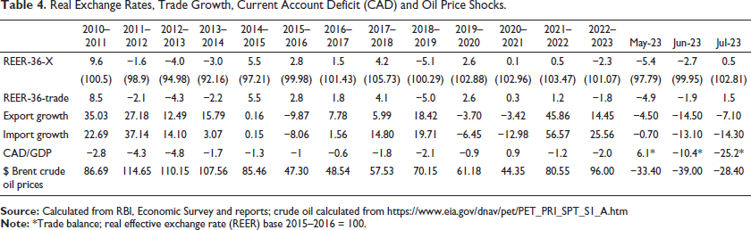
Moreover, impulse responses estimated in Banerjee and Goyal (2021) show the impact of misalignments on current account imbalances to be limited. The majority of research studies find that Indian export growth is normally more sensitive to world growth and demand than to the real exchange rate (Veeramani, 2012). Figure 4 and Table 4 suggest that Indian import and export growth periods coincide with global growth and commodity price cycles. There is no close discernible relationship with REER changes. Export growth has been high in periods when the REER was appreciating as in 2010–2011, but the reverse is also true, as in 2014–2015. However, Goyal and Kumar (2018) find a real appreciation sustained over 2 years or more hurts export growth. REER levels of around 100 since 2018 have been consistent with a sharp rise in export growth. Therefore, sustained appreciation above equilibrium REER levels as occurred over 2015–2018 should be avoided.
Export, Import Growth and the Exchange Rate.
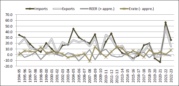
The rupee also cannot appreciate substantially unless the Renminbi does so, since China is a major trade competitor and partner. The dollar has a weight of about 8 per cent in the REER (following the US trade weight) but about 80 per cent of India’s trade (including in fuel oil) is settled in dollars. So the bilateral rate may have more of an impact on trade than the REER, although Figure 4 does not suggest this.
Real Exchange Rates, Trade Growth, Current Account Deficit (CAD) and Oil Price Shocks.
Since depreciation increases costs and inflation given India’s dependence on imported inputs, large competitive depreciations may not result in real depreciation. Indian export growth is better supported by removing supply-side obstacles, improving logistics, marketing, trade standards and ease of doing business, and active diversification of export destinations, combined with a fair-valued REER. The sharp spike in export growth in 2021–2022, a period of global slowdown, was driven by such policy initiatives.
The exchange rate affects the real sector not only from the impact of the real exchange rate on net exports but also its effect on the interest rate. Raising interest rates to defend the rupee from outflows in 2011, 2013 and 2018 went counter to the needs of the investment cycle. In contrast, in 2001 and in 2022 when misalignments in the real exchange rate were minimised and the policy rate was kept near equilibrium, an industrial revival occurred.
Indian exchange rate management deserves praise for avoiding contagion from global crises and managing the pressures of gradually opening the economy without major trauma. But growth sacrifice was higher and more prolonged than necessary in periods such as the 2010s.
Excess Volatility and Risk Premium
Uncovered interest parity (UIP) gives the relationship between expected depreciation and the interest rate differential (IRD) for a country. Under free capital flows and perfect markets, higher interest rates must cover expected depreciation through cross-currency arbitrage. This implies if domestic interest rates rise, the currency jumps up immediately, so the interest rate gap is covered by an expected depreciation. Since UIP involves the exchange rate expected over time, the IRD covers expected depreciation plus a risk or UIP premium.
In covered interest rate parity (CIP), there is no uncertainty since it holds at a point in time. Currency arbitrage should ensure that, for any two countries, the IRD should equal the depreciation of forward currency rates over spot (the forward premium, FP). Table 5 has the annual IRD, FP and depreciation for a few EMs 4 over 2005–2022 with respect to the USD. The IRD in the table is the government bond yield differential over 12-month horizons with respect to the US rates. We see that both the IRD and the FP substantially exceed actual depreciation. China has a positive IRD even though its currency appreciated on average in that period.
Excess Returns in Emerging Markets.
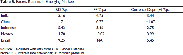
UIP tells us under free capital flows EM nominal interest rates must equal those of the US + expected depreciation + country risk premium. IRD in EMs is always positive and rises with excess exchange rate volatility. The latter is often due to global and not domestic factors. Global interest rate shocks raise capital flow and exchange rate volatility in EMs aggravate EM UIP premia on local-currency debt and raise their borrowing costs (Banerjee & Goyal, 2022). Episodes of sharp depreciation in EMs are not fully offset by appreciation, whereas in AEs, there is more even two-way movement. Even so, IRD over-compensates and exceeds depreciation in EMs. Shocks to the IRDs are usually not offset by realisations of EM depreciation, giving excess returns to foreign investors.
Therefore, EM exchange rates fail to act as a shock absorber, unlike in AEs. The UIP premium is consistently positive. Das et al. (2021) estimate an average positive value of 3 per cent for UIP in EMs. That IRD is found to be consistently higher than FP also for EMs, which exceeds actual depreciation, implies FX markets do not work well and confirms that investors enjoy a significant excess compensation from investing in EM assets (Goyal & Ray, 2023).
It follows a pure float is not the appropriate currency regime for EMs. A higher expected depreciation risk requires IRD to be high for EMs, although that depreciation is only rarely observed in the data. Global investors charge an excess premium from EMs that may be driven by policy uncertainty and expectations of exchange rate fluctuations.
The Indian experience shows it is possible to reduce excess depreciation despite global risk-on and offs. Table 6 gives the mean and standard deviation for Indian 3-month IRD and depreciation with respect to the US over 2004–2022 and two sub-periods. Volatility is measured by the standard deviation of actual depreciation. This rose for most EMs after the GFC but fell for India after 2013.
Indian Exchange Rates and Interest Differentials.
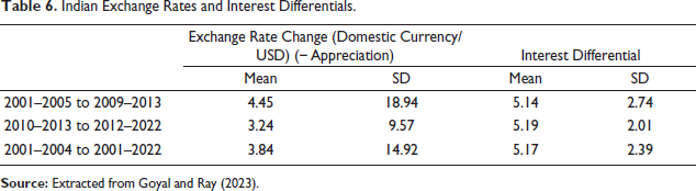
Intervention after 2013 was able to substantially reduce volatility. Over 2014–2017, the mean IRD was 6.9 and the average depreciation was 1.3. After sharp depreciation in 2018, more even two-way nominal movement with middling volatility (Table 2) and stability around competitive real equilibrium exchange rates was established. Over 2019–2022, the mean IRD was 3.4 and the average depreciation was 4.2 despite the pandemic shocks. Risk premiums fell.
Fundamentals were better also: More stable Indian macros, lower inflation differentials and stable growth, among the highest in the world, was reducing country risk premium, as was growing economic size and diversity. Unlike the USA, excess demand or tight labour markets were not driving Indian inflation. There were no second-round effects from supply shocks. Fiscal policies were moderating the latter. The sensitivity to commodity prices had also reduced. Timely regulatory and other relief to the financial sector, as well as its timely withdrawal, had prevented moral hazard, reduced risk and interest rate spreads.
Since the international financial architecture offers hardly any support to EMs, markets tend to have more confidence in countries with self-insurance through large buffers. India’s FX reserves proved a useful counter-cyclical buffer. Figure 5(a) shows reserves increased in most periods but were used when necessary. Reserves dipped in 2008, 2011 and 2022 but were more than made up later. The CAD never fell below 2 per cent of GDP after 2013 while the capital account surplus ratio mostly exceeded 2 per cent.
(a) India’s Balance of Payments (Ratio to GDP). (b) Capital Flows in India.
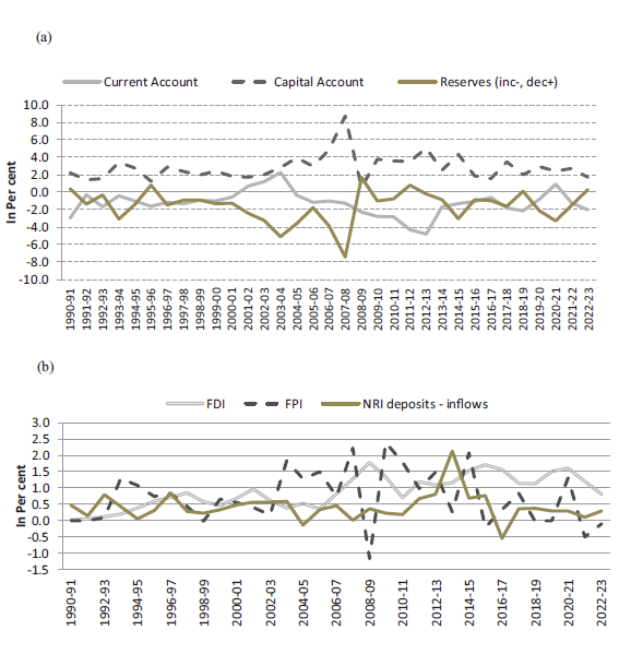
Moreover, interest differential sensitive inflows were still not fully free in India due to its carefully sequenced capital account convertibility. India liberalised equity flows more while retaining graduated restrictions on debt, especially short-term debt, inflows. 5 The rationale was that even though equity flows are volatile they are at least risk-sharing, while debt outflows impose a greater burden in downturns. Restrictions could be tightened when there was a surge in aggregate capital inflows and relaxed when inflows slowed.
Figure 5b shows the increase in foreign direct investment (FDI) and the fluctuations in foreign portfolio investment (FPI). But as a percentage of GDP fluctuations in FPI were lower in the pandemic period although absolute amounts were still large (Figure 6). Higher GDP had increased the absorptive capacity of the economy and its resilience to capital flow surges. Greater participation of households and domestic institutions in equity markets reduced the impact of foreign equity movements on stock market indices. This is an example of how rising economic diversity reduces volatility.
Monthly Equity and Debt Inflows ($ Million).
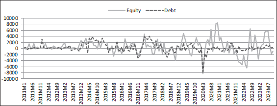
In 2013 and 2017, a rise in Indian policy rates followed Fed tightening. In both periods, Indian market positions were largely long in government debt as interest rates were in a downward phase. As policy raised rates partly to mitigate debt outflows, bond values fell creating large domestic market losses, and shrinking domestic institutional and retail participation in debt, further raising G-sec rates. The economy slowed. But capital affected by UIP was small enough as a share of the market to give monetary policy independence. The share of foreign debt securities has averaged about 8 per cent of total foreign liabilities since 2010, peaking at 11 per cent.
The rise in yields was driven more by unnecessary policy tightening, not the debt outflows, in the Indian context. 6 Post-pandemic experience was different. Although markets expected policy rates to maintain a gap with US Fed rates, there were no major debt outflows in 2022–2023 despite a narrowing interest differential. Total debt capital in India stayed constant at around $100bn during 2023 as the Fed raised rates but the MPC paused. Equity inflows returned even as differentials narrowed (Figure 6). Returns to fixed income flows depend more on currency movements and country risk than on IRD. Rising US Fed rates do lead to safe haven equity outflows from India, but domestic rate rise does not keep them here. It only dampens expectations of growth and therefore induces more equity outflows, and raises country risk-premiums. It is better, therefore, that policy uses the freedoms it has to respond to the needs of the domestic cycle.
Thus, space can be created for domestic policies to counter global shocks. If the domestic exchange rate regime and macroprudential and FX intervention policies lower exchange rate volatility and the country risk premium falls, IRD can fall for an EM, reducing excess returns for foreign investors. Better global safety nets would also help.
Fluctuations in the rupee also absorb some capital flow volatility. Variation of a managed float in a sliding band of about 10 per cent prevents riskless ‘puts’ against the CB, since then there is a substantial risk of loss if the expected movement does not materialise. But intervention when the market-determined level deviates from fundamentals aids market and real stability. Some exchange rate flexibility deepens markets and encourages hedging, but large volatility hurts the real sector.
Two-way nominal movement makes it possible for the exchange rate to also contribute to reducing inflation. Intervention can abort pass-through to inflation from international commodity price shocks as well as exchange rate over-depreciation.
Inflation
If expectations are well-anchored at the inflation target, a temporary cost shock should not have second-round effects. There are signs of such anchoring in India. But since commodities still have a large weight in the CPI headline, the targeted inflation series, an appreciation can also be an antidote to international food and oil shocks, mitigating first-round inflation volatility. Since demand for these commodities is inelastic in the short run, depreciation widens the CAD. After reforms oil marketing companies pass on 7 international variations to domestic pump prices. Farmer lobbies ensure food border prices pass through into domestic procurement prices. Aborting such political bargaining and possible second-round rise in wages and prices could prevent inflation from becoming persistent and resulting in real appreciation.
Depreciation corrects for inflation differentials but itself contributes to inflation. As the costs of imports and import substitutes rise, real depreciation is much lower. A vicious cycle of higher inflation, real appreciation requiring more depreciation can set in. Bouts of a sharp depreciation in 2008, 2011, 2013 and 2018, which were not fully reversed, contributed to sticky Indian inflation, and hardened inflation expectations. After 2011, growth fell while inflation remained high and sticky following the policy combination of a sharp rise in policy rates and sharp depreciation. Excess volatility, even if it is due to a sharp depreciation, does not improve exports. Over 2011–2013, the nominal exchange rate depreciated from 45 to 60, but persistent inflation had converted the real depreciation in 2013 (REER index 105) into a real appreciation (REER index 111) the very next year. Real appreciation reduces export competitiveness. This cannot be ignored when the trade deficit is large.
If the Indian inflation range of 4–5 per cent exceeds that of the rest of the world (range 1–3 per cent), the rupee has to depreciate to the extent a higher productivity differential does not compensate. The mild depreciation required to maintain the REER at equilibrium need not be inflationary, if it is achieved through continuous two-way movements so that sharp depreciations are avoided.
Figure 7 shows 3-year moving averages of changes in the average annual nominal exchange rate, WPI and CPI. It shows a considerable fall in exchange rate fluctuations in recent years with depreciation more closely aligned to inflation rates. In earlier periods, under- or over-correction of the nominal exchange rate sustained occasional overshooting, inflation and misalignment of the real exchange rate. Episodes of large depreciation were linked to external shocks.
Three-Year Moving Averages of Inflation and Change in INR/USD.
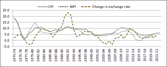
Fuel oil has a higher weight in WPI and food in the CPI. So the first-round impact of an international oil price shock is larger on the WPI. The fluctuation in CPI inflation used to follow that in WPI but in the (post-2015) inflation targeting era, the fluctuation in CPI inflation is less than in WPI, suggesting lower second-round pass through of oil price shocks. Diversification and development are working to reduce vulnerability to international commodity prices. The energy intensity of GDP has fallen. The changing correlation pattern of the USD with oil shocks is a concern, however.
In commodity price booms, the USD used to typically depreciate; when commodity prices fell, it tended to appreciate. Since oil imports are denominated in USD, this reduced the impact of oil price shocks for oil importers such as India. But in the post-pandemic period, the USD appreciated as oil prices rose. Rees (2023) presents evidence that this correlation pattern could become the norm. The reasons are: USD appreciates when the US terms of trade (the ratio of US export prices to US import prices) improve. Before the 2010s, a rise in commodity prices was associated with deterioration in the US terms of trade. But with the shale oil boom higher commodity prices improve the US terms of trade, as the USA is now a net commodity exporter.
So there may be more need to intervene to prevent rupee depreciation when international oil prices rise but the USD strengthens. Now with less overall volatility, finer counter-cyclical movements with the 10 per cent band may be adequate. If there are large outflows, the CB typically comes in after the market bottoms out so portfolio investors share currency risk. The band may, therefore, occasionally be breached but should soon revert.
Our analysis has implications for the optimal exchange rate regime under inflation targeting for EMs. This differs from the textbook recommendation of a full float and is more than the RBI’s preventing excess volatility. It suggests a flexible exchange rate with intervention to prevent excess volatility as well as misalignment from competitive real exchange rates while allowing some volatility to aid price discovery in FX markets. Most EM CBs attempt something like this in practice. But in the presence of capital flow volatility due to global shocks, effective implementation requires the availability and use of multiple instruments.
Large reserves, the absence of full capital account convertibility, use of prudential measures, signals and strategic intervention can help reduce excess volatility of the exchange rate and mismatch of the policy rate from the needs of the domestic cycle. Reducing domestic demand is a costly and inefficient way to respond to the threat of outflows. A larger tool box is an essential defence to continuing global fragilities. But these tools work best with markets if they help them find and maintain the fair value of the currency. The nominal exchange rate has to be flexible.
Although the exchange rate regime established post-liberalisation continued for three decades, implementation and outcomes have varied.
In theory, an exchange rate regime can contribute to multiple objectives including maintaining a real competitive exchange rate, neutralising inflationary oil shocks, deepening FX markets and encouraging hedging.
In the initial decade, there was no two-way movement. FX markets were thin, with many restrictions. Nominal depreciation compensated for higher Indian inflation and maintained a competitive REER. Volatility rose, with a greater role for markets in the 2000s. Two-way nominal movement was established. After the GFC, intervention changed from too little to too much. There was excessive real appreciation.
After the pandemic, the real exchange rate was maintained around equilibrium levels. Despite large outflows, depreciation was orderly. A major achievement was demonstrating that Indian monetary policy had effective independence from US policy, as the interest differential was allowed to narrow, but did not provoke major outflows. Markets easily panicked in EMs and were concerned about the IRD. But good fundamentals and market-based interventions worked together. Risk premiums and interest rate spreads fell.
Depreciation occurred largely in periods of external shocks and outflows, which often coincided with rising international oil prices. Since the dollar now also tends to appreciate in such periods, reversing earlier trends, intervention to prevent excess rupee depreciation and abort pass through to inflation can add value.
Export competitiveness cannot be neglected when the trade deficit is large. Maintaining yet limiting nominal volatility in a 10 per cent band can help markets converge to equilibrium values while reducing risks and giving space for neutralising some international oil shocks. Moderate exchange rate flexibility deepens market and supports exports. The academic literature has also shifted away from advocating corner regimes of a full float or tight fix for EMs towards middling regimes.
Footnotes
Acknowledgement
Declaration of Conflicting Interest
The author declared no potential conflicts of interest regarding the research, authorship and/or publication of this article.
Funding
The author received no financial support for the research, authorship and/or publication of this article.