The Firm’s Role in Displaced Workers’ Earnings Losses

Abstract

The authors investigate the role of firm pay premiums in explaining the large, persistent earnings losses of displaced workers. They first estimate that long-run earnings for displaced workers from 2002 to 2008 in Ohio are depressed by 22%. Drawing upon empirical approaches from the displaced worker and firm heterogeneity literature, the authors then estimate that one-quarter of this earnings loss can be explained by the forfeiture of a favorable employer-specific pay premium. Such firm rents are more salient for those laid off from manufacturing firms, explaining half of their lost earnings. Nevertheless, this study adds to early evidence that firm rents do not explain the majority of earnings losses sustained by displaced workers in the United States.

Keywords

layoffs plant closings wage differentials

Labor economists have long recognized that workers who experience job displacement suffer large and persistent earnings losses for many years after their initial separations—a pattern not exhibited by voluntary job movers. This scarring effect was first documented more than 30 years ago by the seminal work of Jacobson, LaLonde, and Sullivan (1993b) (henceforth JLS) who found that high-tenure workers in Pennsylvania displaced in the early 1980s sustained long-term earnings losses of 25%. Many researchers have since used administrative data to study a range of settings and time periods, all concluding that displacement leads to long-term earnings losses, typically between 15 and 30% (Couch 2001; Jacobson, LaLonde, and Sullivan 2005; von Wachter, Song, and Manchester 2009; Couch and Placzek 2010; Schmieder, von Wachter, and Bender 2010). Davis and von Wachter (2011) found that earnings losses are not only deep and sustained but also highly countercyclical—deficits are twice as large in present-value terms for layoffs when the unemployment rate exceeds 8% than when it is below 6%. Schmieder and von Wachter (2010) showed displacement wipes out workers’ wage gains even during tight labor markets.

The explanation for these persistent earnings losses is less clear. The inability of traditional models used to study unemployment (Mortensen and Pissarides 1994) to capture the magnitude and persistence of earnings losses has motivated research aimed at understanding their sources. Some researchers have posited job ladder models in which workers’ stock of firm-specific human capital increases with tenure, but its value is destroyed upon separation. Unemployed workers are then more likely to search for work in lower-paying, less-stable occupations that differ from their pre-layoff position, leading to large and persistent earning losses (Krolikowski 2017; Huckfeldt 2022; Jarosch 2023). Lachowska, Mas, and Woodbury (2020) focused on the role of productivity-enhancing worker–firm match effects, and they provide evidence that the loss of a favorable firm-specific match is the main driver of persistent scarring.

Another hypothesis for persistent earnings losses involves the firms themselves. Economists have documented that some firms pay higher wages than others for equally skilled workers, a conclusion bolstered by the proliferation of studies using employer–employee matched data (Bronars and Famulari 1997; Abowd, Kramarz, and Margolis 1999; Card, Heining, and Kline 2013; Song et al. 2018). Sustained earnings losses could arise if workers are systematically displaced from high-pay premium firms and subsequently hired and retained by employers offering lower pay premiums.¹

Several papers use administrative data and the Abowd, Kramarz, and Margolis (1999) (henceforth AKM) methodology to investigate this channel. In the German context, two papers found that long-run wage losses of 11 to 15% are nearly fully explained by the forfeiture of firm wage premiums, implying little role for other channels (Fackler, Mueller, and Stegmaier 2021; Schmieder, von Wachter, and Heining 2023). Evidence from Portugal found a somewhat smaller penalty for displacement (approximately 7%) and found a smaller but still non-trivial role for firm fixed effects, which the authors find explains about 27% of earnings losses (Raposo, Portugal, and Carneiro 2021). In stark contrast, the only extant study in the United States found that firm premiums play a minimal role in explaining earnings losses (Lachowska et al. 2020). Using data on displacements during the Great Recession, the authors conclude that the firm-specific component of pay accounts for just 9% of overall earnings losses. They instead attribute most of the losses to forfeited job-specific matches—time-invariant factors that forge a particularly valuable employee–employer pairing—and residual displacement effects, such as loss of seniority (52% and 39% of losses, respectively).

Given these contrasting findings, a natural question is whether the minimal role of firm pay premiums found by Lachowska et al. (2020) generalizes to the United States more broadly. With that motivation, we use employer–employee matched administrative data from Ohio to investigate the role of firm pay premiums in explaining losses of displaced workers. Specifically, we implement AKM on a comprehensive panel of Ohio workers to estimate firm-specific pay premia. In contrast to previous literature, we include the pre-layoff earnings of displaced workers in AKM estimation, rather than excluding them entirely. Our rationale, which we test in sensitivity analyses, is that if displaced workers are fully excluded from the AKM estimation, the resulting firm fixed effects may not fully reflect what these workers stand to lose in a subsequent displacement.

After presenting our main findings, we interpret the results alongside prior work (particularly Lachowska et al. 2020), seeking to reconcile the differences to the extent feasible. Further work is needed to determine why the magnitude of the effect varies across regions.

Data

The state of Ohio requires all employers, as part of the state’s unemployment insurance (UI) payroll tax requirements, to report quarterly earnings for all employees. We use two Ohio administrative data sources to study the links between displacement and firm-specific pay premiums. These data are made available through the Ohio Education Research Center (OERC), which assembles data from multiple state agencies, including the Ohio Department of Job and Family Services (ODJFS), into a repository known as the Ohio Longitudinal Data Archive (OLDA).²

The first data set includes information on both firms and private sector, state, and local public employees subject to UI contributions in Ohio between 1999Q3 and 2013Q1. Thus, an observation exists for every quarter an individual has positive earnings at a covered employer in the state of Ohio during this time period. Individual identifiers allow us to classify the quarter of a displaced worker’s separation and subsequent employment over time.

The second data set includes firm-level variables such as an anonymized employer identifier, three-digit North American Industry Classification Systems (NAICS) codes, and county of the employer. The identifiers allow for construction of a firm-size variable by summing across the records associated with a given employer in each quarter. The firm identifiers are consistent across the two data sets, allowing us to link firms and workers.

The Ohio administrative data are particularly advantageous for the purposes of studying displaced workers’ earnings patterns. Ohio is the seventh largest US state by population and lies at the heart of America’s manufacturing region, which has experienced several decades of de-industrialization. Relative to other states, Ohio has large employment shares in manufacturing, a sector more likely to produce displaced workers. Like the rest of the United States, Ohio experienced recessions in 2001–2002 and 2008–2009, time frames included in our sample period.

Our data have several limitations. First, we are unable to distinguish between workers who leave Ohio, drop out of the labor force, or begin working for non-UI-covered employers in the state.³ Second, UI administrative records rarely include demographic characteristics and collect characteristics only on workers who ultimately claim unemployment insurance (UI). We do not impose that our sample of displaced workers claim UI benefits, given that take-up among eligible US workers is roughly 50% (Anderson and Meyer 1997; Lachowska, Sorkin, and Woodbury 2023). Such a restriction would omit a substantial share of the population of interest. Thus, our sample lacks demographic information.

We use the Ohio administrative records to construct two distinct samples: one for implementing the AKM approach to estimate firm-specific pay premia, or “firm fixed effects,” and a considerably smaller sample for analyzing the earnings losses of displaced workers. We describe the sample used for AKM estimation and the displaced worker sample in the Empirical Approach sections below.

Empirical Approach

Our approach begins with the AKM model, which we use to identify firm-specific pay premiums for Ohio employers. We then employ a standard multi-period difference-in-difference model to infer the causal effect of displacement on earnings. Our approach of leveraging estimated firm fixed effects seeks to understand the role the firm plays in displaced worker earnings losses.

AKM Model

The increased prevalence of matched employee–employer administrative data sets has enhanced the quality and quantity of research on both displaced workers and firm-specific pay premiums. In their seminal research on the French labor market, AKM documented that workers who move between establishments experience wage gains or losses in a highly predictable manner, providing credibility to the claim that “where you work” matters for “what you earn.” Using matched employer–employee data, AKM developed the following model for log earnings of person i working at firm j in year t:

l o g {(e a r n)}_{i j t} = α_{i} + γ_{t} + θ_{j (i, t)} + ε_{i j t}

(1)

In Equation (1), α_i are worker fixed effects, which capture the component of earnings that moves with a worker regardless of her employer. The θ_j_(i,t) represent firm fixed effects,⁴ reflecting the earnings premium or penalty (relative to some omitted firm) associated with working at firm j. The γ_t are year fixed effects, and ε_ijt is an unobserved time-varying error that may capture shocks to human capital, individual-job match effects, or other transitory shocks. We estimate Equation (1) on the universe of 1999–2012 Ohio workers from the UI data (subject to certain sample restrictions described later in this section). We then use the ${\hat{θ}}_{j}$ estimates that correspond to each firm in subsequent analysis to estimate the effect of losing firm pay premia.

To separately identify α_i and θ_j_(i,t) in Equation (1), there must be sufficient movement of workers between firms to form a “connected set.” Specifically, firms whose workers have not moved to or from other establishments during the length of the panel are not linked to other employers by worker transitions and are thus not part of the connected set. Such firms without any movers are inevitable in such a large data set, but in practice they do not substantially reduce the size of the connected set, meaning the AKM estimates should be trustworthy for the population. As illustrated in Online Appendix Table A.1, 89% of all workers and 88% of all firms are included in the largest connected set from the Ohio sample.⁵ (Note that hereafter, numbering for Online Appendix material is prefaced with an “A.,” such as Appendix A.4, Table A.1, and so forth.)

In Appendix A.4, we provide a variance decomposition of log earnings for Equation (1) and show 24 to 25% of the variation can be explained by firm fixed effects in various Ohio samples. This value compares to 22% estimated by Sorkin (2018), 21% in Card et al. (2013), and 20% in Lachowska et al. (2020).

While we believe the AKM model accurately describes the wage structure across firms and workers and provides a valuable estimate of firm premiums, it does not perfectly describe the labor market. The static nature of AKM imposes that worker mobility does not depend on prior employment history, suggesting a worker’s “origin firm” does not matter for her wage at a destination firm (Di Addario, Kline, Saggio, and Sølvsten 2023).

AKM Sample Construction

The AKM sample is constructed from the Ohio quarterly earnings records for calendar years 1999 to 2012. Because the data do not include hours worked and we seek to approximate firm-specific earnings premiums paid to full-time employees, we drop worker-quarter observations when a worker has two or more listed jobs. We then follow the method developed by Sorkin (2018) of constructing an employee–employer matched panel to study worker movements. Specifically, we subset on continuous spells of employment that last for at least five consecutive quarters to eliminate short-term and seasonal employees. For each employment spell with a distinct employer, we drop the first and last quarter of the spell to avoid making inferences about earnings based on partial quarters of employment.

Because the AKM model is traditionally estimated on yearly panels rather than quarterly, we follow Lachowska et al. (2020) and annualize the remaining data within each calendar year and multiply the mean quarterly earnings by four to reflect annual earnings (conditional on a worker having two consecutive quarters of earnings from the same primary employer). If this condition is not met, the year for that individual worker is omitted. We also drop worker-year observations when average yearly earnings are below $3,500, given such observations likely reflect less than part-time work for any substantial span of time.

Such restrictions are sufficient for many papers that employ AKM (Song et al. 2018; Sorkin 2018). However, because we use the estimated firm premiums for displaced worker analysis, further sample restrictions are necessary. Specifically, we drop worker-year observations for displaced workers for the years of and after layoff. We do not want to estimate firm-specific pay premiums that are a function of the very earnings changes we seek to partially attribute to lost firm premiums. Including such observations would violate AKM’s identifying assumptions, because if the scarring effect of displacement is caused even partially by factors unrelated to firm premiums (e.g., loss of seniority, loss of a good match, etc.), post-layoff earnings are not, in expectation, the simple sum of individual and firm fixed effects. See Appendix A.1 for further discussion.

While dropping all observations from ever-displaced workers is a reasonable alternative approach to this issue in AKM estimation, we opt to drop only post-displacement worker-year observations out of a concern that dropping displaced workers entirely may understate the estimated firm fixed effects.⁶ Displaced workers have lower estimated worker fixed effects within their firms. (We document this fact in Appendix A.3.) Thus, their omission from the sample would mean the fixed effects of layoff firms are estimated from a set of higher-fixed-effect workers, potentially understating the contribution of the firm premiums to the remaining workers’ pay. This would, in turn, understate the role of the firm in the long-term earnings losses of displaced workers (both in share and in absolute magnitude). In our Results section, we illustrate that this choice indeed ultimately affects the estimation of the share of total earnings losses that can be explained by firm premiums. These restrictions yield the preferred “full sample” from column (1) of Table A.1. On this sample, we estimate firm fixed effects using the largest connected set, that is, the greatest collection of workers and firms linked by worker movements over time.⁷

JLS Model

Before investigating the role of firm-specific wage premiums in explaining displaced worker earnings losses, we must first estimate the simple effects of displacement on workers’ overall earnings. We do so by estimating the following multi-period difference-in-difference specification:

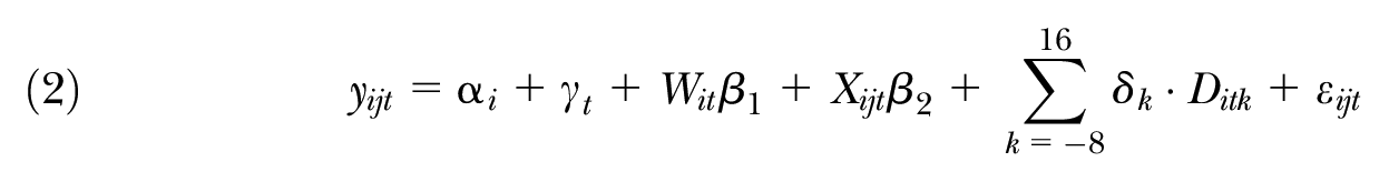
y_{i j t} = α_{i} + γ_{t} + W_{i t} β_{1} + X_{i j t} β_{2} + \sum_{k = - 8}^{16} δ_{k} \cdot D_{i t k} + ε_{i j t}

(2)

In Equation (2), y_ijt are the log of quarterly earnings for worker i in quarter t at firm j; α_i and γ_t are worker and year-quarter fixed effects, respectively; X_ijt includes a vector of two-digit NAICS code dummies for worker i’s layoff employer j (or the comparison worker’s primary employer) interacted with a vector of yearly indicators; and W_it is a vector of yearly indicators interacted with pre-displacement earnings (average of the 5–8 quarters before separation for treatment group, average of 2003 earnings for comparison group), allowing for the possibility that workers with different pre-earnings may have different trends over time. Covariate D_itk is an indicator that equals one if worker i is observed in quarter k relative to displacement in calendar-quarter t, and equals zero otherwise. In the final quarter of a displaced worker’s observed tenure with the layoff employer, k assumes the value zero. The δ_k term represents the baseline displacement effect on earnings in quarter k relative to separation. Because the within-worker residuals cannot be assumed to be independent across time, we cluster at the worker level. Last, because “Ashenfelter dips” (drops in earnings that precede displacement) can affect earnings despite displacement not having yet occurred, we allow the index k to assume negative values as low as −8. Since each displaced worker has at least three years of tenure, the “omitted category” for the treated sample includes earnings in quarters −12 ≤ k ≤−9.

To interpret δ_k as the causal effect of displacement on earnings, the parallel trends assumption—that displaced and non-displaced worker earnings would have followed the same trend in absence of treatment—must be met. According to Equation (2), the specified treatment begins eight quarters prior to displacement, so earnings between the two groups must be parallel in the third year prior to separation. Displaced workers, by definition, are highly tenured at the time of their layoff, so we require the comparison group of stably employed workers be similarly high-tenured.⁸ Even if the high-tenured workers in the comparison group are not comparable to the displaced sample along certain unobservables (such as ability or productivity), so long as the gap between the treatment and control workers is constant prior to treatment and would have remained constant absent displacement, the δ_k coefficients can be interpreted as causal.

Construction of Displaced and Comparison Samples

Because we use administrative data, we cannot explicitly identify the reason for a worker’s separation (quit, discharge for cause, etc.). Consistent with the displaced worker literature, we use separations during a mass layoff between 2002Q1 and 2008Q4 to identify workers who separate because of economic distress at the firm.⁹ Mass layoffs serve as a reliable proxy for causes of displacement because most workers who leave a firm during such a period do so involuntarily.

Following Davis and von Wachter (2011), we define a mass layoff as a 30% or more quarter-to-quarter reduction in a firm’s employment level. A firm shutdown is counted as a mass layoff. Because some firms exhibit many mass layoffs, we rank a firm’s four largest mass layoffs by percentage change during the relevant period (2002–2008) and assess only these four events to avoid overcounting. Further, as smaller firms are mathematically more likely to meet this 30% benchmark without a substantial change in absolute employment, we adhere to JLS’s practice of excluding firms with fewer than 50 employees from the sample of mass layoff firms.

Upon identifying the various dates of a firm’s mass layoffs, we define a displaced worker as someone satisfying the following conditions: The individual 1) is employed at the firm within a year prior to a given mass layoff, 2) is not employed at the firm the quarter after the mass layoff, 3) exhibits at least three years’ tenure at the layoff firm, 4) holds only one job at the time of job separation, and 5) earns at least minimum wage corresponding to 30 hours per week.¹⁰ While this definition closely aligns with JLS, we impose a tenure requirement of three years rather than the six years JLS used. This less stringent requirement, also followed by Davis and von Wachter (2011), allows us to study a greater number of displaced cohorts.¹¹ As a robustness check, we test the sensitivity of our estimates to a more common tenure requirement of six years at the layoff employer.

Further, because our research question—understanding the share of earnings losses attributable to loss of a firm pay premium—necessitates that a displaced worker will seek future employment, it does not make sense to study those who may drop out of the labor force altogether. As a baseline, we follow much of the displaced worker literature and require that all displaced workers in our sample stay somewhat attached to the labor force in the follow-up period, defined as exhibiting positive earnings in at least 25% of one’s post-displacement quarters.¹² In Appendix B, we explore sensitivity of our results to this requirement by conditioning on higher attachment (more post-displacement quarters of positive earnings). Given this sample restriction, our conclusions about displaced workers are conditional on labor force attachment.

Last, consistent with JLS and similar papers, we compare the outcomes of our displaced sample to a control group of workers who remain continuously employed. Traditionally, the literature has predominantly used a “never displaced” control group to isolate the portion of earnings potential that is destroyed when an individual involuntarily loses a specific job (Krolikowski 2018).

Descriptive Statistics

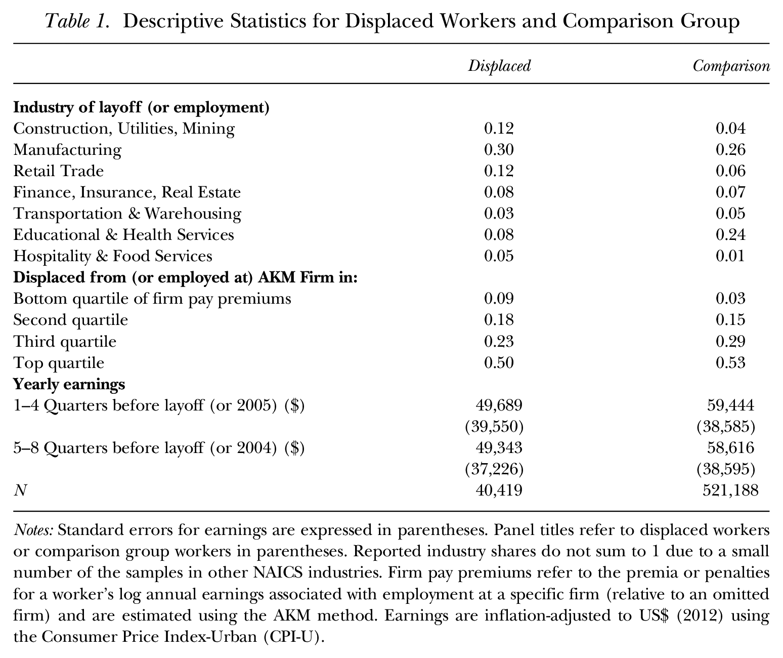
Table 1 summarizes key variables for the sample of workers displaced in Ohio between 2002Q1 and 2008Q4 and the stably employed comparison sample used in our difference-in-difference model. The comparison group, who are highly tenured at the same firm throughout the panel, outnumber the displaced workers by a ratio of 13:1. Such a large sample size for the comparison group is instrumental in producing the precise regression-adjusted estimates that will be presented in the Results section. Half of all comparison workers are employed in either manufacturing or education and health services, a combined share similar to the comparison group from Lachowska et al. (2020).

Table 1.

Descriptive Statistics for Displaced Workers and Comparison Group

	Displaced	Comparison
Industry of layoff (or employment)
Construction, Utilities, Mining	0.12	0.04
Manufacturing	0.30	0.26
Retail Trade	0.12	0.06
Finance, Insurance, Real Estate	0.08	0.07
Transportation & Warehousing	0.03	0.05
Educational & Health Services	0.08	0.24
Hospitality & Food Services	0.05	0.01
Displaced from (or employed at) AKM Firm in:
Bottom quartile of firm pay premiums	0.09	0.03
Second quartile	0.18	0.15
Third quartile	0.23	0.29
Top quartile	0.50	0.53
Yearly earnings
1–4 Quarters before layoff (or 2005) ($)	49,689 (39,550)	59,444 (38,585)
5–8 Quarters before layoff (or 2004) ($)	49,343 (37,226)	58,616 (38,595)
N	40,419	521,188

Notes: Standard errors for earnings are expressed in parentheses. Panel titles refer to displaced workers or comparison group workers in parentheses. Reported industry shares do not sum to 1 due to a small number of the samples in other NAICS industries. Firm pay premiums refer to the premia or penalties for a worker’s log annual earnings associated with employment at a specific firm (relative to an omitted firm) and are estimated using the AKM method. Earnings are inflation-adjusted to US$ (2012) using the Consumer Price Index-Urban (CPI-U).

A similar share of displaced and comparison workers come from the top quartile of firm-specific pay premiums, although a slightly larger share of displaced workers come from lower-quartile firms. The comparison group has significantly higher pre-layoff earnings (defined as 2004–2005 earnings, which is the median layoff time period) than the displaced sample, but we argue this will not threaten identification using the difference-in-difference strategy.

Table 1 also shows that 30% of the displaced worker sample were laid off from manufacturing firms, which is unsurprising given Ohio’s industrial base. The composition of displaced workers in the Ohio sample is similar to the primary displaced sample in Washington State from Lachowska et al. (2020) (28%). However, the manufacturing share contrasts with the displaced sample JLS analyzed from 1980s Pennsylvania that included many more from manufacturing (75%), while those analyzed by Couch and Placzek (2010) (early 2000s Connecticut) were less concentrated in manufacturing (16%).

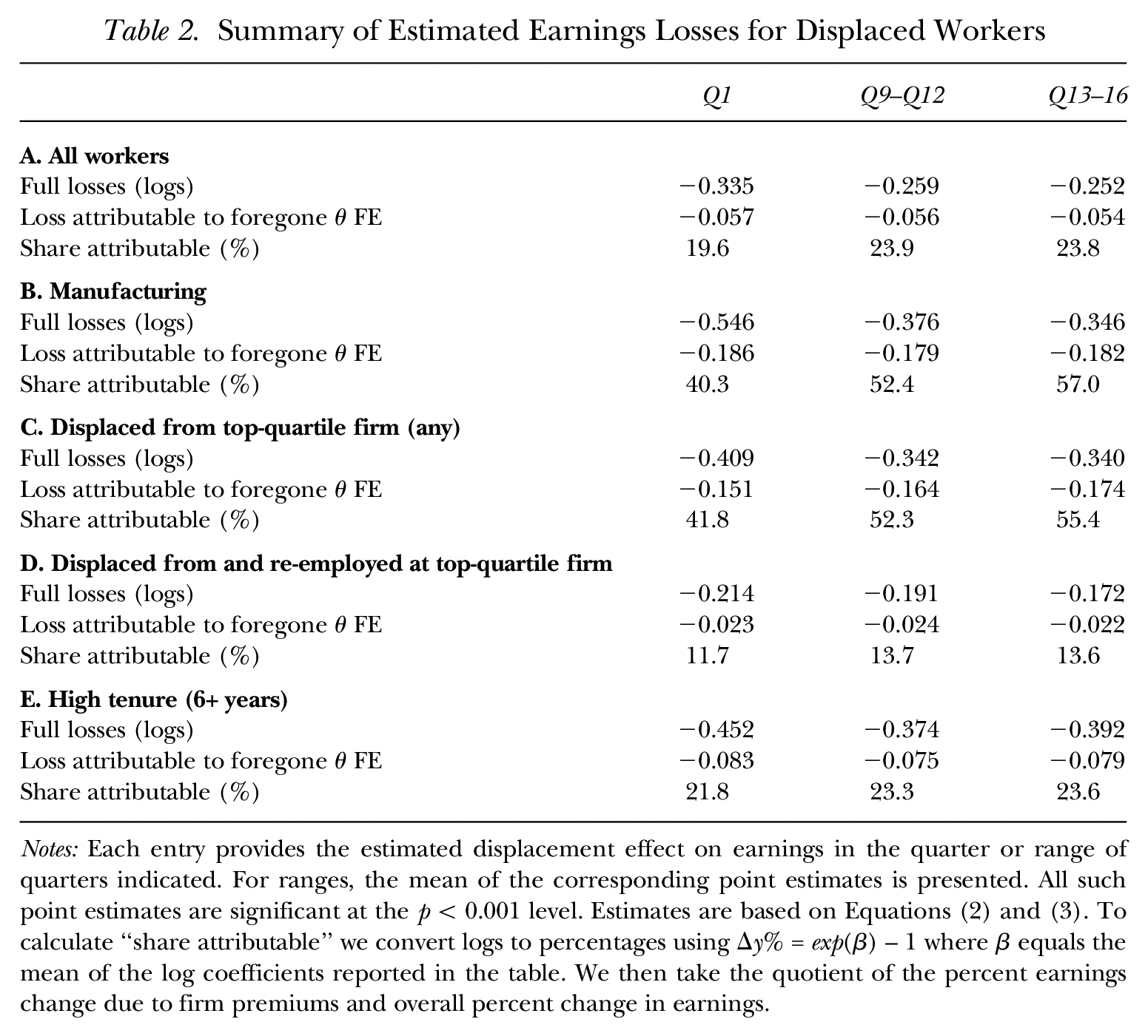
The bottom two panels of Table 1 (firm premium quartile and pre-displacement yearly earnings) show that the average displaced worker earned roughly $50,000 in the year before separation, and half of them separated from a firm in the top-quartile of employer pay premiums. These statistics are similar to those generated by Lachowska et al. (2020). The earnings of workers two years before displacement are only slightly lower than earnings the year before, indicating a relatively minimal Ashenfelter dip compared to the early displaced worker literature. Figure 1 likewise indicates no dip before displacement. This finding of a limited Ashenfelter dip is consistent with displaced worker earnings profiles of more recent work using administrative data by Hyman (2018) and Braxton, Herkenhoff, and Phillips (2020).

Figure 1.

Earnings Profile of Displaced and Non-Displaced Workers

To illustrate the validity of the parallel trends assumption in this context, we plot the earnings of displaced workers and the comparison group before and after their separation date (see Figure 1).¹³ From three years prior to displacement up to the date of separation, the mean quarterly earnings of the displaced and non-displaced cohorts follow the same common trend. Even before regression adjustment, the persistent earnings losses are apparent up to four years after displacement. This figure provides supporting evidence that if no such displacement occurred to the treated sample, the earnings of the two groups would have continued growing at the same pace, suggesting Equation (2) is well-identified.

JLS-AKM Model

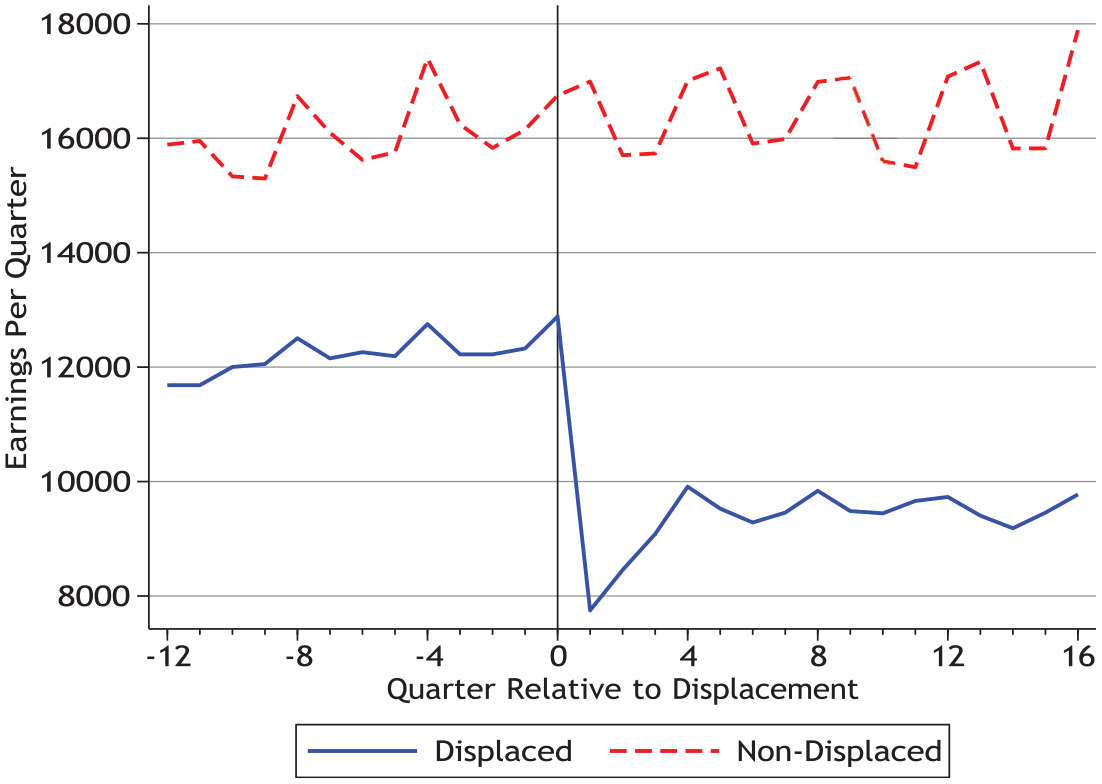
To assess the role of firm-specific pay premiums in the earnings losses of displaced workers, we follow Lachowska et al. (2020) and treat the previously estimated employer fixed effects ${\hat{θ}}_{j}$ as an additional outcome in the displacement process. We match the $\hat{θ}$ ’s obtained from estimating Equation (1) to the worker-quarter observations that correspond to the proper firm identifier in the displaced and comparison groups summarized in Table 1. Specifically, displaced worker i at firm j in year-quarter t is assigned a corresponding value for ${\hat{θ}}_{j (i, t)}$ —her firm-specific pay premium that partially determines earnings—which varies only when she switches employers. All individuals, including displaced workers, have a ${\hat{θ}}_{j (i, t)}$ for the entire panel while employed.¹⁴

We use these estimated firm effects as a left-hand side variable in the following regression, modeled after Equation (2):

{\hat{θ}}_{j (i, t)} = α_{i} + γ_{t} + W_{i t} β_{1} + X_{i j t} β_{2} + \sum_{k = - 8}^{16} ω_{k} \cdot D_{i t k} + ν_{i j t}

(3)

Note that the right-hand sides of Equations (2) and (3) are identical, meaning the same difference-in-difference reasoning applies. The parallel trends assumption for Equation (3) is particularly straightforward: Because the displaced sample is required to be employed at the same firm during the pre-treatment period (quarters 9 through 12 before layoff), then ${\hat{θ}}_{j}$ , which changes for worker i only when she moves firms, remains constant in the pre-period. Workers in the comparison group, who never change employers, possess a constant firm-specific pay premium throughout the panel.

The estimated ω_k’s are thus the effect of displacement on the firm-specific component of earnings for worker i in quarter k relative to displacement. In effect, each ω_k estimates

E [θ_{j} | α_{i}, γ_{t}, D_{i t k} = 1] - E [θ_{j} | α_{i}, γ_{t}, D_{i t k} = 0]

where D_itk equals one if a displaced worker is observed in a post-separation quarter, and zero if a displaced worker pre-separation or a stably employed worker is observed. A negative ω_k for positive values of k would provide evidence of lost employer-specific premiums. The quotient of the ω_k coefficient and δ_k from Equation (2) approximates the share of earnings losses attributable to lost firm fixed effects k quarters after displacement.¹⁵

Results

Estimates of Lost Earnings

The first row of panel A in Table 2 summarizes the estimates of short- and long-term earnings losses for the full sample of 40,419 Ohio workers displaced between 2002Q1 and 2008Q4. In the first full quarter after displacement, workers’ earnings decrease by 34 log points. Observations in which workers experience zero earnings for a quarter are dropped from the regression. This approach is because we seek to understand how forfeited firm premiums explain earnings losses, so we do not want to consider losses that result from working for no firm at all. Thus, the presented coefficients provide estimates of the effect of displacement conditional on employment.¹⁶ Because many who find re-employment in the quarter after displacement may work only a partial quarter, it is likely that this drastic drop is driven substantially by reduced work hours over the quarter. Of greater interest are long-run earnings effects, which we spend the remainder of the article examining.

Table 2.

Summary of Estimated Earnings Losses for Displaced Workers

	Q1	Q9–Q12	Q13–16
A. All workers
Full losses (logs)	−0.335	−0.259	−0.252
Loss attributable to foregone θ FE	−0.057	−0.056	−0.054
Share attributable (%)	19.6	23.9	23.8
B. Manufacturing
Full losses (logs)	−0.546	−0.376	−0.346
Loss attributable to foregone θ FE	−0.186	−0.179	−0.182
Share attributable (%)	40.3	52.4	57.0
C. Displaced from top-quartile firm (any)
Full losses (logs)	−0.409	−0.342	−0.340
Loss attributable to foregone θ FE	−0.151	−0.164	−0.174
Share attributable (%)	41.8	52.3	55.4
D. Displaced from and re-employed at top-quartile firm
Full losses (logs)	−0.214	−0.191	−0.172
Loss attributable to foregone θ FE	−0.023	−0.024	−0.022
Share attributable (%)	11.7	13.7	13.6
E. High tenure (6+ years)
Full losses (logs)	−0.452	−0.374	−0.392
Loss attributable to foregone θ FE	−0.083	−0.075	−0.079
Share attributable (%)	21.8	23.3	23.6

Notes: Each entry provides the estimated displacement effect on earnings in the quarter or range of quarters indicated. For ranges, the mean of the corresponding point estimates is presented. All such point estimates are significant at the p < 0.001 level. Estimates are based on Equations (2) and (3). To calculate “share attributable” we convert logs to percentages using Δy% = exp(β) – 1 where β equals the mean of the log coefficients reported in the table. We then take the quotient of the percent earnings change due to firm premiums and overall percent change in earnings.

Four years after displacement, workers earn approximately 25.2 log points less on average than they would have if they were not displaced.¹⁷ Converting log points to percentage terms, we estimate long-term earnings for displaced workers are about 22% less than their pre-displacement earnings [exp(−0.252) – 1]. Such estimates fall well within the bounds of the recent displaced worker literature.¹⁸ Figure 2 plots the baseline displaced worker earnings losses profile for up to four years after job loss.¹⁹ The short- and long-term effects of displacement are negative and highly significant. Noticeably, the causal effects of displacement on earnings relative to quarter of separation follow the familiar “dip, drop, and partial recovery” pattern. For robustness, we run Equation (2) without controlling for the level of a displaced worker’s pre-layoff earnings (see Table B.2). We find a nearly identical earnings profile and estimate earnings losses of 21%.

Figure 2.

Regression-Adjusted Estimates of Earnings Losses Due to Displacement

The magnitude of these long-run earnings loss estimates for Ohio workers are on the upper end of, but not outside, the bounds of previous literature. Jacobson, Lalonde, and Sullivan (1993a) documented losses on the order of 25%. Our estimates are somewhat larger than Lachowska et al. (2020) for Washington or Schmieder et al. (2023) for West Germany (15–16%), and they are significantly larger than those documented in Portugal by Raposo et al. (2021) (7%).

Also worth noting is that these long-run earnings losses for workers who separated between 2002Q1 and 2008Q4 are quite substantial given their time of displacement in the business cycle. Ohio’s unemployment rate²⁰ stayed below 6% for the majority of the 28 total quarters. However, the 2000’s expansion may be an exception to Davis and von Wachter's (2011) finding that long-run earnings losses of displaced workers are mitigated when the labor market is strong. The authors also noted that the 2003–2005 period—when US unemployment was below 6%—was an anomaly, as high-tenured men displaced during these years exhibited long-run earnings losses greater than those displaced at any other time in the previous quarter-century (including losses sustained by those displaced in the 1982 recession, when unemployment eclipsed 9%).

We conduct the same analysis on a subset of displaced workers that may experience earnings patterns that differ from the overall sample: those displaced from manufacturing. We are interested in manufacturing in particular because of our attractive setting to study the industry. During our layoff window from 2002 to 2008, the number of workers in manufacturing decreased drastically by 22% in Ohio compared to 11% nationally. Our time frame also coincides with the brunt of the post-WTO accession “China shock.” Rubber and glass manufacturing—among the most exposed industries to Chinese imports in the early 2000s, as detailed by Autor, Dorn, and Hanson (2013)—were heavily concentrated in Ohio.

Table 2, panel B summarizes earnings losses associated with displacement from manufacturing firms. These deficits are markedly larger than those of the rest of the sample. They exhibit 55 log point earnings losses in the first quarter after separation. Strikingly, even four years after displacement, they earn 29% (34.6 log points) less than they would have if they were not displaced, conditional on employment.²¹ These long-run estimates hover around the largest estimates in the literature for all displaced workers, which consistently measures losses between 15 and 30% in a diverse set of labor market contexts.

Estimated Losses Due to Firm Fixed Effects

According to Table 1, roughly half of displaced workers separate from firms in the top quartile of pay premiums and very few separate from the bottom quartile. If displaced workers are systematically re-employed by firms that offer a lower pay premium to all employees, then a portion of the earnings losses described in the Estimates of Lost Earnings section above can be explained by this downward transition to lower θ_j firms. We approach this question using model (3) equation.

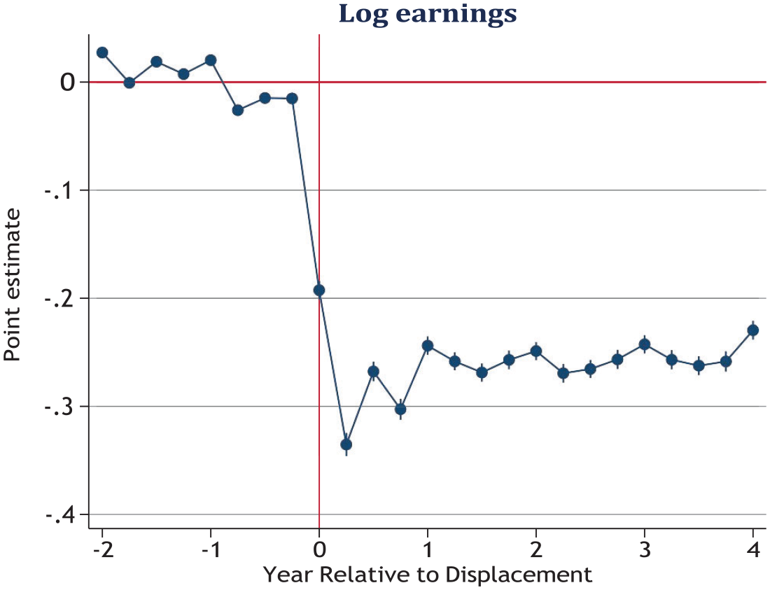
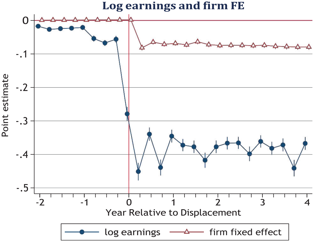
Figure 3 plots the estimated δ_k and ω_k from regression Equations (2) and (3) for quarter k relative to displacement, −8 ≤ k ≤ 16. These represent the estimated displacement effects on log earnings and employer-specific pay premiums, respectively. Results show that 16 quarters after displacement, average worker earnings are roughly five log points lower than they would be absent a layoff because of re-employment at a firm with a lower pay premium. The second row of panel A in Table 2 provides the average point estimates for the short- and long-term effects of displacement on the firm-specific component on earnings. We document that firm effects alone decrease long-run earnings for displaced workers by 5.4 log points.

Figure 3.

Estimated Displacement Losses Due to Foregone Employer Fixed Effects (FE)

We can calculate the share of losses explained by dividing the percentage earnings losses attributable to firm pay premiums by overall earnings deficits. These statistics are presented in the third rows of each panel of Table 2. For the overall sample, approximately 24% of a worker’s earnings deficits four years after displacement are attributable to employment at firms with lower pay premiums. Laid-off manufacturing employees can attribute more than half of their sizable long-run earnings losses to forfeited firm-specific pay premiums. Strikingly, the earnings deficits for displaced manufacturing employees deriving from loss of a favorable firm premium nearly match the magnitude for the overall earnings losses for the general sample. These results are consistent with Helm, Kügler, and Schönberg (2022), who likewise documented a large role for firm effects in displacement from manufacturing in Germany. Charts similar to Figure 3 for these two subsets of displaced workers, as well as tables of point estimates and standard errors, can be found in Appendix B (Figure B.5, Table B.5, and Table B.6).

Within manufacturing, we next explore subsectors that are heavily concentrated in Ohio. Specifically, we restrict our displaced and comparison samples to those laid off from (or employed in) NAICS three-digit sectors 325–327. These include producers of chemicals (including synthetic rubbers), rubber, plastic, and glass. Workers laid off from these narrow sectors account for 20% of our manufacturing sample (or 5% of our overall sample).²² Figure B.6 illustrates that when we restrict the sample to these “Ohio-specific” manufacturing sectors, the role for firm effects increases. Four years after displacement, earnings losses for these workers are around 38 log points, with 25 log points attributable to firm fixed effects. This finding means that for these workers, approximately 66% of losses are explained by firm fixed effects, compared to 57% for the manufacturing sector more broadly and 24% for the sample overall.

Our main results follow a practice of nearly all displaced worker articles using administrative data by conditioning that workers have positive earnings in 25% of post-displacement quarters (and positive earnings in at least one quarter of every post-layoff calendar year). As a robustness check on our finding that firm premiums explain one-quarter of overall earnings losses, we subject our sample to more stringent requirements of post-layoff attachment. While both the overall earnings losses and losses due to firm premiums shrink with more stringent requirements of 50% and 75% attachment, the share of losses attributable to firm effects remains remarkably stable around 25%. (Point estimates are provided in Appendix B, Table B.3, Figure B.3, and Figure B.4.)

Workers Displaced from Top AKM Quartile Firms

Given a large share of our sample is displaced from firms offering a top-quartile pay premium, we estimate Equations (2) and (3) on the subsample of displaced workers who lost a job from a top quartile firm and a comparison group of workers at such a firm. Their earnings losses are shown in Figure B.7a and summarized in Table 2, panel C. After four years, they earn 34 log points less than they would have absent a layoff. Not only are losses for these workers larger than for the overall sample but also deficits are greater in absolute terms, given they earn nearly $10,000 more per year pre-layoff.

Table 2, panel C, also suggests such workers intuitively have “more to lose” by separating from their employer: We attribute half of their total earnings deficits to loss of a favorable firm-specific pay premium. For this group, earnings are depressed by 15 to 16% by firm effects alone. The overall earnings deficits, losses due to firm premiums, and the share of losses due to premiums are all comparable to figures for the manufacturing subsample, even though two-thirds of this group separated from an industry other than manufacturing. This observation suggests the importance of firm pay premiums not being limited to manufacturing layoffs.

Roughly 25% of our displaced sample separates from high- ${\hat{θ}}_{j}$ (top-quartile) firms but finds re-employment at another top-quartile firm (see Appendix B, Figure B.2). Even for this “lucky” group of laid-off workers, displacement tends to lead to re-employment at lower-paying firms on average. Table 2, panel D, shows that these workers suffer 16 log point long-run earnings deficits. As expected, a smaller than average share (13%) is attributable to receiving a lower pay premium, but the firm effect of displacement still persists.²³

Sensitivity of Estimates to Sample Construction

The JLS-AKM framework necessarily involves many precise decisions about sample restrictions for both stages of estimation. Related studies that use UI administrative records from US states vary in how they construct their preferred displaced sample (Jacobson et al. 1993b; Couch and Placzek 2010; Ost, Pan, and Webber 2018; Lachowska et al. 2020). Further, researchers using the JLS-AKM framework can reasonably exclude workers designated as displaced from the sample to which AKM is applied. Thus, the resulting ${\hat{θ}}_{j}$ estimates from Equation (1)—and in turn, the share of firm premiums on earnings losses—may vary substantially with small adjustments in the sample restrictions.

We explore how our estimates change with constructions of different samples and if it could account for disagreement between past work on the role of firm rents. Fackler et al. (2021) and Schmieder et al. (2023) concluded that firm premiums are either the sole or overwhelming source of displaced worker earnings losses in Germany. Similar to our main result, Raposo et al. (2021) found that firm premiums explain approximately 27% of overall losses. Whereas Lachowska et al. (2020) found that for workers in Washington State during the Great Recession, firm effects depress long-run earnings by 1.5%, accounting for just 9% of overall losses.

AKM Sensitivity

As a robustness check, we adjust the construction of the economy-wide AKM sample to which Equation (1) is applied. As discussed earlier in the AKM Sample Construction section, AKM is typically estimated on the entire sample of workers and firms to maximize the size of the largest connected set. Because we use the estimates of ${\hat{θ}}_{j}$ for subsequent analysis, however, we drop post-layoff observations of displaced workers (but retain pre-layoff observations) from AKM under the argument that dropping displaced workers entirely could lead to skewed estimates of firm premiums ${\hat{θ}}_{j}$ by omitting workers with lower fixed effects. Another approach to this issue (as followed by Lachowska et al. 2020) is to go further and omit all displaced and comparison group worker-year observations from the sample which they estimate using AKM. Either approach could plausibly satisfy the AKM identifying assumptions. To assess how much this choice matters, we test the sensitivity of our estimates to alternative AKM sample construction.²⁴

We find that estimated losses due to firm premiums, and thus the share of overall deficits they explain, are sensitive to AKM sample selection. Figure 4 plots results from Ohio for firm premium losses using two different AKM sample constructions. Omitting comparison and displaced workers altogether reduces our estimated earnings losses attributable to firm premiums by as much as one-third. Because overall estimated earnings losses do not depend on firm fixed effects resulting from the AKM sample, the corresponding share explained by pay premiums likewise declines with the use of the alternative AKM sample, from 24% to 16%.

Figure 4.

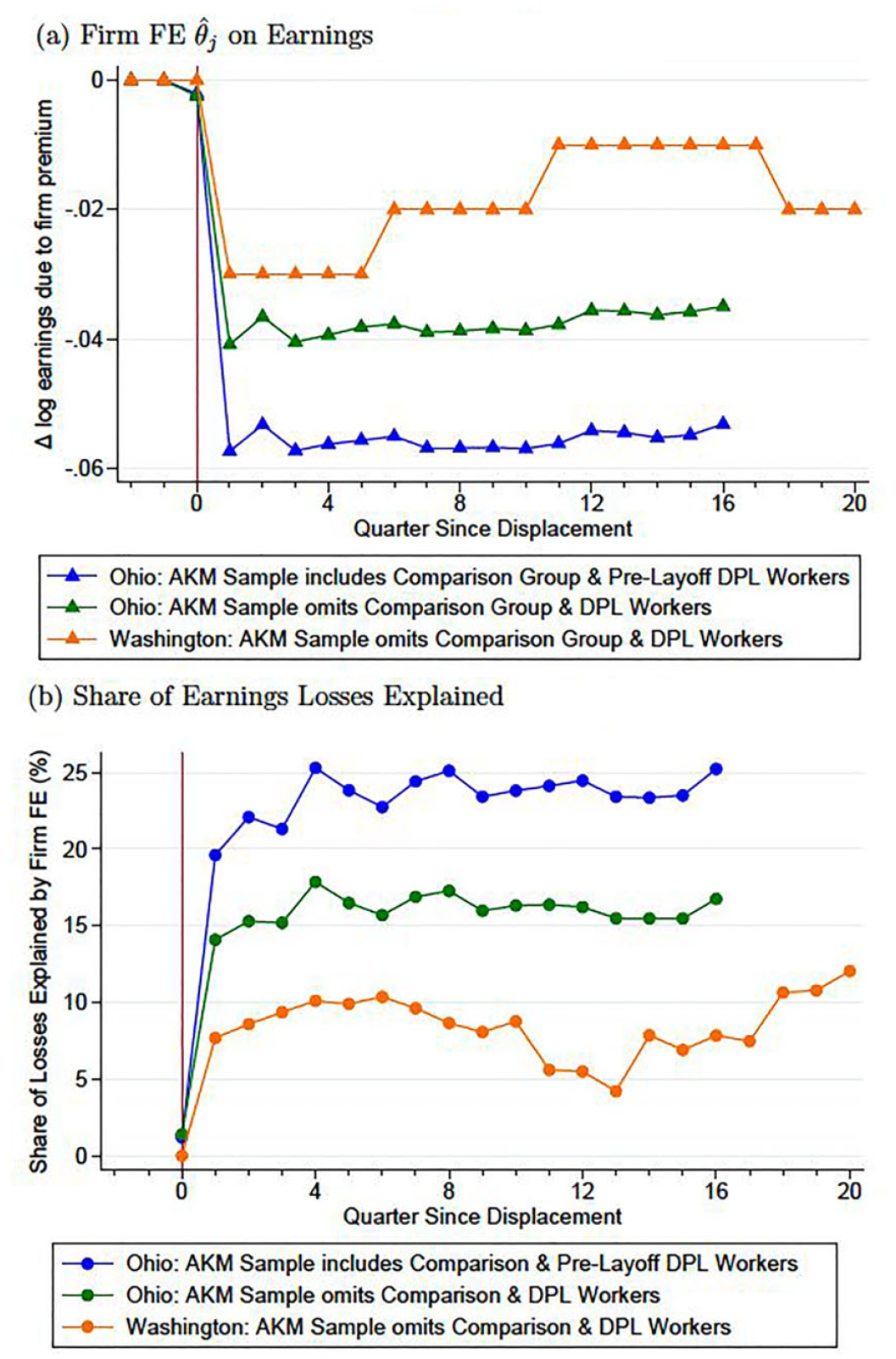
Earnings Losses Due to Foregone Firm Fixed Effects (FE) Based on AKM Sample Selection: Ohio and Washington Estimates

The sensitivity shown in Figure 4 suggests that when displaced and comparison workers are omitted from the AKM sample, either the estimated ${\hat{θ}}_{j}$ for layoff firms are lower, or estimated ${\hat{θ}}_{j}$ for firms that hire newly displaced workers are higher (or both). We find evidence for the former case. Estimated fixed effects for mass layoff employers are larger for our preferred AKM sample than for the alternative sample (see Appendix A). The same relationship holds for the difference between the estimated firm fixed effects of layoff firms and non-layoff firms. The result is robust to various definitions of “layoff firm.”²⁵

The reason for this sensitivity in estimated firm premiums to the AKM sample construction reflects the fact that displaced workers have lower estimated worker fixed effects ${\hat{α}}_{i}$ than do workers who remain at their firm after a layoff. Following Gulyas (2016), in Figure A.2 we present a binscatter of average change in a firm’s employment against the firm’s average worker quality for firms that rapidly contract. We find that firms that contract by 35% or more quarter-to-quarter experience a statistically significant increase in their average worker quality, suggesting the workers they shed had lower values of ${\hat{α}}_{i}$ . This dynamic has implications for estimation of ${\hat{θ}}_{j}$ for layoff firms in particular: When the AKM sample omits displaced workers entirely (rather than including their pre-layoff observations), estimated ${\hat{α}}_{i}$ ’s of incumbent workers are biased upward, thereby depressing the estimated firm premiums. While both sample constructions are valid for the JLS-AKM framework, we prefer our sample because estimation includes pre-layoff displaced workers, who have lower values of ${\hat{α}}_{i}$ . In any case, while this choice has non-trivial consequences for assessing the role of firm fixed effects in explaining earnings losses for displaced workers, it does not radically change the estimate.

Comparison to Previous Estimates

Our finding that firm rents explain only 24% of long-run earnings losses bolsters Lachowska et al.’s (2020) conclusion that such premiums are not the primary cause of earnings scarring for workers in the United States (just 9%). However, our estimates are more than twice as large as their results and suggest a more pronounced role for firm rents. A key difference in our empirical approach involves AKM construction as described above in the AKM Sensitivity section.²⁶ Adjusting the AKM sample attenuates our estimate in Lachowska et al.’s (2020) direction, as illustrated by Figure 4. The difference in AKM sample selection appears to account for roughly half the difference between our estimates and Lachowska et al.’s (2020). The difference in the other direction between our Ohio estimates and Schmieder et al.’s (2023) estimates from Germany are not explained by AKM sample or tenure requirements, however, because both articles follow the same sample construction.

Figure 5.

Estimated Displacement Effects on Earnings: Overall and Due to Foregone Employer Fixed Effects (FE); Six Years Tenure

Beyond the difference in AKM construction, important institutional factors likely explain the remaining difference in our estimates. For example, while all the workers in Lachowska et al. (2020) are displaced during the Great Recession, the bulk of workers in our study separate during a tight labor market. If losses resulting from forgone firm premiums are acyclical, such premiums may explain a relatively smaller share of overall losses during an economic downturn compared to an expansion because total earnings deficits are larger during a recession (Davis and von Wachter 2011). And yet, there are various reasons to believe displaced workers forfeit a different kind of firm premium over the business cycle. For example, large employers, which offer well-documented wage premiums (Brown and Medoff 1989; Bloom et al. 2018) and are less sensitive during economic downturns than their smaller counterparts (Gertler and Gilchrist 1994; Fort, Haltiwanger, Jarmin, and Miranda 2013), displace a greater share of all laid-off workers in business cycle peaks than in troughs.²⁷ Indeed, Schmieder et al. (2023) provided evidence that the magnitude of earnings losses deriving from firm premiums in Germany are countercyclical.

To investigate whether the business cycle may account for our estimates being moderately larger than those of Lachowska et al. (2020), we plot the average pay premium of layoff firms in Ohio against the state’s unemployment rate in Figure 6. Although most workers we analyze are displaced in a tight labor market, our layoff window extends to the eve of the Great Recession in 2008.²⁸ Both the unweighted and employment-weighted average pay premium of layoff firms in Ohio appear to drop as the labor market improves. 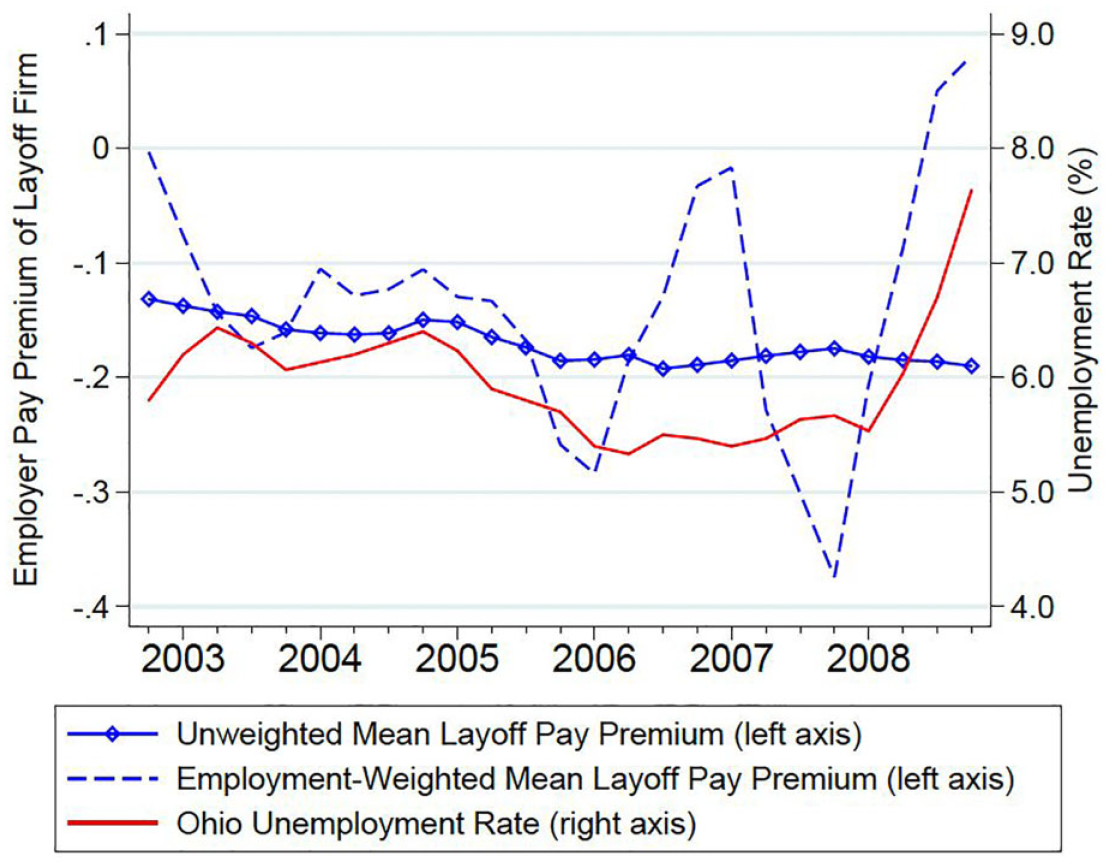But, as the unemployment rate spikes in 2008, the employment-weighted mean ${\hat{θ}}_{j}$ of layoff firms likewise rises markedly. If this series moves with the unemployment rate throughout the business cycle, it could suggest firm premiums would explain even more than one quarter of long-run earnings losses, rather than less. In other words, the difference in time periods between our analysis and Lachowska et al. (2020) does not appear to explain the larger estimates we find.

Figure 6.

Average Layoff Firm Premium and Ohio Unemployment Rate

Another possible explanation is the difference in industry mix between Ohio and Washington. While the share of workers who are displaced from manufacturing does not vary between the Ohio and Washington samples (27%), it may be that rubber, plastic, or glass manufacturing plants of Ohio confer a more generous pay premium than the types of manufacturers concentrated in Washington State. If manufacturing employees in Ohio forfeit a larger firm-specific wage premium than those in Washington, on average, this could explain at least part of the remaining gap between our estimates. While we believe Figure B.6 provides suggestive evidence for this claim, the fact we do not have access to the Washington data means we cannot answer this definitively.

Conclusion

Highly tenured displaced workers suffer large and persistent earnings losses many years after their initial separations, the sources of which have long been a puzzle for labor economists. We first verify that workers in Ohio displaced in the mid-2000s have similar experiences, earning 22% less than they otherwise would have four years after displacement. Losses are substantially larger for those shed from manufacturing firms. We then seek to address one potential driver of earnings scarring by showing that firm-specific pay premiums explain a meaningful share of overall displaced worker earnings losses in Ohio, although they are not the primary source. Specifically, we show long-run earnings of workers who lose their job in a mass layoff are lower by 5.3% due exclusively to the loss of a favorable firm pay premium. This finding accounts for 24% of long-run earnings losses. For those separating from manufacturing firms, premium forfeiture leads to earning losses of 17%, explaining more than half of long-run deficits.

Our preferred AKM sample construction includes pre-displacement earnings observations for displaced workers. On average, such workers have lower average worker fixed effects, such that excluding them completely from the AKM sample may understate the role of firm-specific rents. Indeed, we find that excluding these workers attenuates our estimate for the share of the earnings scar attributable to firm effects from 24 to 16%, accounting for roughly half the difference in the “share explained” estimates between our study and Lachowska et al. (2020).

We further explore the implications of differences in settings, comparing mid-2000s Ohio to Washington during the Great Recession. Data limitations prevent us from investigating how losses due to firm premiums change with fluctuations in the unemployment rate. Nonetheless, our data suggest such losses would, if anything, increase for workers laid off during a downturn, which is consistent with Schmieder et al.’s (2023) findings for Germany but does not help to explain our larger estimates than Lachowska et al. (2020). While both states displace a similar proportion of workers from the manufacturing sector, we provide suggestive evidence that firm fixed effects may play a particularly large role in some manufacturing subsectors that are more concentrated in Ohio. While our estimates for losses due to firm premiums and the share of overall deficits they explain are still more than twice as large as evidence from Washington, they are still broadly consistent with Lachowska et al.’s (2020) findings that firm premiums play a much smaller role in the United States than in Germany. Whether employer pay premiums explain one-sixth or one-quarter of long-run earnings losses, it implies other factors—among them, skill depreciation while unemployed, loss of seniority, and forfeiture of positive match effects—are all potential sources of the remaining share of the earnings scar.

Our analysis leaves several open questions for future work. In particular, it would be useful to further explore the role of match effects, particularly in settings where firm effects themselves play a larger role in earnings losses. Additional work is also needed to study how firm premiums in the United States change over the business cycle and how this could affect outcomes for workers who lose their job during an economic downturn. Workers laid off during a recession differ on numerous dimensions from those displaced during an expansion. The same is true for firms that shed workers at different points in the cycle. A framework such as JLS-AKM, which describes the cost of job loss, would ultimately want to account for such changes in worker and firm composition over the business cycle.

Supplemental Material

sj-pdf-1-ilr-10.1177_00197939241310124 – Supplemental material for The Firm’s Role in Displaced Workers’ Earnings Losses

Supplemental material, sj-pdf-1-ilr-10.1177_00197939241310124 for The Firm’s Role in Displaced Workers’ Earnings Losses by Brendan Moore and Judith Scott-Clayton in ILR Review

Footnotes

Acknowledgements

We thank Katharine Abraham, Michael Best, Carter Braxton, Bruce Fallick, Ben Hyman, Gregor Jarosch, Wilbert van der Klaauw, Marta Lachowska, Rasmus Lentz, Bentley MacLeod, Suresh Naidu, Christina Patterson, Jesse Rothstein, Aysegül Şahin, and Jim Spletzer for feedback on earlier drafts of this article. We gratefully acknowledge Lisa Neilson and the staff of the Ohio Education Research Center, who helped facilitate our use of the restricted data in this study.

ORCID iD

Brendan Moore

An Online Appendix is available at .

For general information or data and/or computer programs, please contact the corresponding author, Brendan Moore, at bdmoore@stanford.edu.

1

Graham, Kim, Li, and Qiu (2019) illustrated a specific mechanism for layoff risk involving firm premiums. Using data from the U.S. Census Bureau, the authors calculate the implied wage premium demanded by workers of a firm with a greater risk of bankruptcy, since highly leveraged firms are also more likely to shed employees.

2

Ohio Longitudinal Data Archive (OLDA) is a project of the Ohio Education Research Center (OERC) (http://www.oerc.osu.edu/oerc.osu.edu) and provides researchers with centralized access to administrative data. The OLDA is managed by The Ohio State University’s CHRR (https://chrr.osu.edu/chrr.osu.edu) in collaboration with Ohio’s state workforce and education agencies (http://www.ohioanalytics.gov/ohioanalytics.gov), with those agencies providing oversight and funding. For information on OLDA sponsors, see .

3

This constraint is typical for displaced worker papers that use administrative data. Although 10% of all displaced workers move as a result of their layoff (), we consider such individuals who leave the state as unattached to the labor force and exclude them from our analysis. If such individuals recoup more of their pre-layoff earnings or find re-employment at higher-paying firms than fellow displaced workers who stay put, our estimates of the magnitude of losses may be biased upward.

4

An estimated ${\hat{θ}}_{j}$ resulting from is constant for a given firm, thus θ could be applied a subscript of j alone. However, because Equation (1) describes worker i’s earnings in time t as a function of her employer’s pay premium, and recognizing workers change employers, we subscript θ with j as a function of i and t.

5

In the extreme case of no worker movement between firms during the panel, the connected set would have zero workers or firms. A connected set including roughly 90% of workers and firms is typical of other papers using the AKM model, such as Card, Heining, and Kline (2013), Card, Cardoso, Heining, and Kline (2018), and .

6

Including pre-displacement observations of displaced workers enables their work history to contribute to broader model estimation. This is the case even for the minority of displaced workers in the sample who do not switch firms prior to layoff (and thus do not contribute to identification of the firm fixed effect).

7

We distinguish between displaced workers’ wages from pre-layoff years and post-layoff years, including the former and excluding the latter in AKM estimation. The year of layoff is always excluded from AKM estimation. Given we do not document any Ashenfelter dip in earnings for the overall sample, concerns that a displacement effect could contaminate earnings in pre-layoff years in AKM are limited. An alternative approach would be to omit the entire year before the displacement year from the AKM estimation.

8

Specifically, a worker must be employed at the same firm for at least 56 of the observed 57 quarters to qualify for the comparison group.

9

Flaaen, Shapiro, and Sorkin (2019) examined the implications of assuming mass layoffs are a sound proxy for economic distress at the firms by matching administrative data sets with the Survey of Income and Program Participation (SIPP) and Longitudinal Employer Household Dynamics (LEHD), both of which contain worker-provided reasons for separations. The authors found that earning loss estimates using only survey responses are very close to those using only administrative data.

10

Quarterly earnings corresponding to the minimum wage (in 2014 inflation-adjusted dollars) is $2,163 in the quarter before displacement. This corresponds to earning $5.15/hour, Ohio’s minimum wage from 2002–2006, for 30 hours per week for one quarter.

11

A small share (8%) of our displaced sample suffer multiple displacements between 2002 and 2008. We analyze these workers’ first displacement and consider later layoffs a subsequent outcome of initial job loss.

12

This baseline sample restriction shrinks our displaced worker sample size by only 8%.

13

In , because the comparison group necessarily lack a separation date, we set the median quarter of displacement for the treated group as their date of separation. For the treated group, the date of separation varies for each displaced worker.

14

A very small share of displaced workers are unmatched to a ${\hat{θ}}_{j}$ because one of their employers (either the layoff or the destination firm) was not in the connected set used to estimate .

15

As will be discussed in the Results section, we prefer to translate the coefficients (in log points) to percentages and take their ratio. Although the difference is slight, it can be more meaningful for large magnitudes and more accurately reflects the desired quantity of interest—what share of earnings losses are due to forfeited firm premiums.

16

While we considered using the inverse hyperbolic sign or changing zero earnings to ones to avoid an undefined log(0) value, we opted against doing so because it would prevent constructing a “share attributable to firm fixed effects” comparisons like that in , which only makes sense when the mapping of quarterly earnings to quarterly firm-specific fixed effects is defined for all earnings.

17

Throughout the article, we refer to figures four years post-displacement to mean the average of the coefficients for quarters 13–16 relative to separation.

18

Lachowska et al. (2020) estimated long-run earnings losses of 15 log points (14%) whereas estimated 32 log points (27%). Both articles define the long run as five years rather than four.

19

A table of point estimates and standard errors for Figure 2 is found in , column (3). Column (1) of this table shows point estimates of the same regression without controlling for pre-earnings interacted with year dummies.

20

Aggregating monthly rates at a quarterly frequency.

21

Point estimates for the effect of displacement on earnings for all quarters are presented in .

22

According to the U.S. Bureau of Labor’s Quarterly Census of Employment and Wages, in 2005 these sectors accounted for just 5.7% of Washington’s manufacturing employment and 0.5% of total wage and salary employment.

23

Graphs of the total and firm effect losses for both of the “top-quartile” displaced groups are presented in .

24

The variance decomposition of log earnings is very similar across various AKM samples, as shown in .

25

compares estimated firm premiums by layoff status.

26

Our sample also differs from Lachowska et al. (2020) in that they impose longer tenure for displaced workers. In Figure 5 and we document this discrepancy is inconsequential for the “share explained” estimates, which are similar for samples with a minimum of three and six years of tenure.

27

According to the Job Openings and Labor Turnover Survey (JOLTS) Experimental Firm Size Class Statistics from the , firms with more than 500 employees accounted for 46% of all employee layoffs in 2017 as opposed to 36% in 2010.

28

We are unable to analyze multiple year cohorts of workers displaced in the Great Recession (2008–2010) using JLS-AKM because our follow-up period would be cut short of four years.

References

Abowd

John M.

Kramarz

Francis

Margolis

David N.

1999. High wage workers and high wage firms. Econometrica 67:251–333.

Anderson

Patricia M.

Meyer

Bruce D.

1997. Unemployment insurance takeup rates and the after-tax value of benefits. Quarterly Journal of Economics 112:913–37.

Autor

David

Dorn

David

Hanson

Gordon H.

2013. The China syndrome: Local labor market effects of import competition in the United States. American Economic Review 103:2121–68.

Bloom

Nick

Guvenen

Fatih

Smith

Ben S.

Song

Jae

von Wachter

Till

. 2018. The disappearing large-firm wage premium. AEA Papers and Proceedings 108:317–22.

Braxton

J. Carter

Herkenhoff

Kyle F.

Phillips

Gordon M.

2020. Can the unemployed borrow? Implications for public insurance. NBER Working Paper No. 27026. Cambridge, MA: National Bureau of Economic Research.

Bronars

Stephen G.

Famulari

Melissa

. 1997. Wage, tenure, and wage growth variation within and across establishments. Journal of Labor Economics 15:285–317.

Brown

Charles

Medoff

James

. 1989. The employer size-wage effect. Journal of Political Economy 97:1027–59.

Bureau of Labor Statistics, U.S. Department of Labor. 2018a. Current Population Survey Displaced Workers Supplement. Accessed August 16, 2019, https://www.bls.gov/news.release/disp.nr0.htm

Bureau of Labor Statistics, U.S. Department of Labor. 2018b. Experimental JOLTS Firm Size Class Statistics. Accessed July 14, 2019, https://www.bls.gov/jlt/jlt_ firmsize.htm

10.

Card

David

Cardoso

Ana Rute

Heining

Joerg

Kline

Patrick

. 2018. Firms and labor market inequality: Evidence and some theory. Journal of Labor Economics 36:S13–S70.

11.

Card

David

Heining

Joerg

Kline

Patrick

. 2013. Workplace heterogeneity and the rise of West German wage inequality. Quarterly Journal of Economics 128:967–1015.

12.

Couch

Kenneth A.

2001. Earnings losses and unemployment of displaced workers in Germany. Industrial and Labor Relations Review 54:559–72.

13.

Couch

Kenneth A.

Placzek

Dana W.

2010. Earnings losses of displaced workers revisited. American Economic Review 100:572–89.

14.

Davis

Steven J.

von Wachter

Till

. 2011. Recessions and the costs of job loss. Brookings Papers on Economic Activity 42:1–72.

15.

Di Addario

Sabrina

Kline

Patrick

Saggio

Raffaele

Sølvsten

Mikkel

. 2023. It ain’t where you’re from, it’s where you’re at: Hiring origins, firm heterogeneity, and wages. Journal of Econometrics 233:340–74.

16.

Fackler

Daniel

Mueller

Steffen

Stegmaier

Jens

. 2021. Explaining wage losses after job displacement: Employer size and lost firm wage premiums. Journal of the European Economic Association 19:2695–736.

17.

Flaaen

Aaron B.

Shapiro

Matthew D.

Sorkin

Isaac

. 2019. Reconsidering the consequences of worker displacements: Firm versus worker perspective. American Economic Journal: Macroeconomics 11:193–227.

18.

Fort

Teresa C.

Haltiwanger

John

Jarmin

Ron S.

Miranda

Javier

. 2013. How firms respond to business cycles: The role of firm age and firm size. IMF Economic Review 61:520–59.

19.

Gertler

Mark

Gilchrist

Simon

. 1994. Monetary policy, business cycles, and the behavior of small manufacturing firms. Quarterly Journal of Economics 109:309–40.

20.

Graham

John R.

Kim

Hyunseob

Qiu

Jiaping

. 2019. Employee costs of corporate bankruptcy. NBER Working Paper No. 25922. Cambridge, MA: National Bureau of Economic Research.

21.

Gulyas

Andreas

. 2016. Identifying labor market sorting with firm dynamics. Manuscript. University of Mannheim, Germany.

22.

Helm

Ines

Kügler

Alice

Schönberg

Uta

. 2022. Displacement effects in manufacturing. Manuscript. Department of Economics, Ludwig-Maximilian University of Munich, Germany.

23.

Huckfeldt

Christopher

. 2022. Understanding the scarring effect of recessions. American Economic Review 112:1273–310.

24.

Hyman

Benjamin G.

2018. Can displaced labor be retrained? Evidence from quasi-random assignment to trade adjustment assistance. January 10. Accessed at https://ssrn.com/abstract=3155386 or http://dx.doi.org/10.2139/ssrn.3155386

25.

Jacobson

Louis

LaLonde

Robert J.

Sullivan

Daniel

. 1993a. The Costs of Worker Dislocation. Kalamazoo, MI: W.E. Upjohn Institute for Employment Research. https://doi.org/10.17848/9780585282992

26.

Jacobson

Louis

LaLonde

Robert J.

Sullivan

Daniel

. 1993b. Earnings losses of displaced workers. American Economic Review 83(4):685–709.

27.

Jacobson

Louis

LaLonde

Robert J.

Sullivan

Daniel

. 2005. The impact of community college retraining on older displaced workers: Should we teach old dogs new tricks? Industrial and Labor Relations Review 58:398–415.

28.

Jarosch

Gregor

. 2023. Searching for job security and the consequences of job loss. Econometrica 91:903–42.

29.

Krolikowski

Pawel

. 2017. Job ladders and earnings of displaced workers. American Economic Journal: Macroeconomics 9:1–31.

30.

Krolikowski

Pawel

. 2018. Choosing a control group for displaced workers. ILR Review 71:1232–54.

31.

Lachowska

Marta

Mas

Alexandre

Woodbury

Stephen A.

2020. Sources of displaced workers’ long-term earnings losses. American Economic Review 110:3231–66.

32.

Lachowska

Marta

Sorkin

Isaac

Woodbury

Stephen A.

2023. Firms and unemployment insurance take-up. NBER Working Paper No. 30266. Cambridge, MA: National Bureau of Economic Research.

33.

Mortensen

Dale T.

Pissarides

Chris A.

1994. Job creation and job destruction in the theory of unemployment. Review of Economic Studies 61:397–415.

34.

Ost

Ben

Pan

Weixiang

Webber

Douglas

. 2018. The impact of mass layoffs on the educational investments of working college students. Labour Economics 51:1–12.

35.

Raposo

Pedro

Portugal

Pedro

Carneiro

Anabela

. 2021. The sources of the wage losses of displaced workers: The role of the reallocation of workers into firms, matches, and job titles. Journal of Human Resources 56:786–820.

36.

Schmieder

Johannes F.

von Wachter

Till

. 2010. Does wage persistence matter for employment fluctuations? Evidence from displaced workers. American Economic Journal: Applied Economics 2:1–21.

37.

Schmieder

Johannes F.

von Wachter

Till

Bender

Stefan

. 2010. The long-term impact of job displacement in Germany during the 1982 recession on earnings, income, and employment. IAB Discussion Paper 1/2010. Institut für Arbeitsmarkt- und Berufsforschung (IAB), Nürnberg Institute for Employment Research, Nuremberg, Germany.

38.

Schmieder

Johannes F.

von Wachter

Till

Heining

Jörg

. 2023. The costs of job displacement over the business cycle and its sources: Evidence from Germany. American Economic Review 113:1208–54.

39.

Song

Jae

Price

David J.

Guvenen

Faith

Bloom

Nicholas

von Wachter

Till

. 2018. Firming up inequality. Quarterly Journal of Economics 134:1–50.

40.

Sorkin

Isaac

. 2018. Ranking firms using revealed preference. Quarterly Journal of Economics 133:1331–93.

41.

von Wachter

Till M.

Song

Jae

Manchester

Joyce

. 2009. Long-term earnings losses due to mass layoffs during the 1982 recession: An analysis using US administrative data from 1974 to 2004. Unpublished Paper. Columbia University, New York.

Supplementary Material

Please find the following supplemental material available below.

For Open Access articles published under a Creative Commons License, all supplemental material carries the same license as the article it is associated with.

For non-Open Access articles published, all supplemental material carries a non-exclusive license, and permission requests for re-use of supplemental material or any part of supplemental material shall be sent directly to the copyright owner as specified in the copyright notice associated with the article.

0.00 MB

1.34 MB