Unpacking the relationship between child poverty rates and educational deprivation: The role of school social composition and public education spending

Abstract

This study examines the relationship between societal child poverty and students’ risk of educational deprivation and explores the underlying mechanisms. Analyzing PISA (Programme for International Student Assessment) 2018 data from 32 countries, we find a positive association that persists even after controlling for individual-level compositional differences. Public education spending, which is negatively associated with child poverty, partly explains this relationship; in other words, countries with higher child poverty rates do not offset the risk of educational deprivation through higher school funding. The main explanation, however, lies in school social composition: high-poverty countries have a larger number of schools with elevated shares of socially disadvantaged students, rather than a higher concentration of disadvantaged students in a few schools, as previous US research has assumed. Overall, our findings suggest that poverty at any level—individual, school, or national—harms children’s educational opportunities, and that schools alone cannot overcome educational deprivation.

Keywords

child poverty educational poverty cross-national comparison PISA public education spending school segregation

Introduction

Across the OECD (2024), nearly one in eight children lives in income poverty, with important cross-country differences. Among the countries included in our study, child poverty—defined as the share of children aged 0–17 living in households with equivalized disposable incomes below 50% of the national median¹—ranges from 3.6% in Finland to 24.7% in Romania (see “Data and methods” section, Table 1). Research shows that experiencing poverty during childhood has detrimental effects on various life outcomes, including health and wellbeing (Chzhen et al., 2021; Ponnet, 2014), cognitive development (Justice et al., 2019; McLoyd et al., 2017; Schoon et al., 2010), and educational achievement/attainment (Duncan et al., 1998; Murnane, 2007). While existing research on the impact of child poverty on educational achievement has predominantly focused on individual-level exposure (Engle and Black, 2008), the influence of prevailing child poverty at the national level remains underexplored (Hannum and Xie, 2017). A better understanding of how societal child poverty affects children’s educational outcomes, beyond their individual experience of poverty, would provide additional avenues for addressing low educational achievement. This is important because improvements in the national average achievement typically result from raising the “floor”—that is, reducing the proportion of low achievers—rather than from improvements among high performers only (OECD, 2016).

To our knowledge, only Condron et al. (2024) explicitly investigate the educational consequences of national child poverty rates, demonstrating that increases in child poverty within countries reduce the country’s (aggregated) academic achievement. However, because their study relies on country-level indicators, it cannot rule out the “simple” explanation that countries with higher child poverty rates have more children living in poverty, who are at greater risk of (very) low achievement. Moreover, the study examines neither why countries’ child poverty rates affect children’s learning outcomes nor whether high child poverty rates are only detrimental to poor children. The latter is particularly important because higher national levels of child poverty are associated with greater income inequality and residential segregation—factors linked to poorer overall educational outcomes (Chmielewski, 2019; Reardon et al., 2024; Solga, 2014; Wodtke et al., 2011; Workman, 2022, 2023). These conditions may hinder learning not only for poor children, but also for non-poor children through school- and classroom-level spillovers (Borgna et al., 2019; Condron, 2011; Merry, 2013; Orfield and Lee, 2005).

Against this background, our study focuses on the risk of educational deprivation as a qualitatively distinct form of low educational achievement rather than merely an educational disadvantage (see below). We propose and test two theoretically grounded—though not exhaustive—explanations for why national child poverty is associated with children’s risks of educational deprivation: differences in the social composition of schools and levels of public education spending. By examining these two plausible mechanisms, our cross-national study extends Condron et al.’s (2024) study and advances our understanding of how societal child poverty hinders educational outcomes. We test these mechanisms using the 2018 PISA (Programme for International Student Assessment) data from 32 countries and three‑level mixed‑effects linear probability models.

In doing so, our study makes four contributions. First, we conceptualize educational deprivation² as “the level of education that is insufficient for participating in labor markets or in social life” (Solga, 2014: 271; see also Allmendinger and Leibfried, 2003) and operationalize it as scoring below proficiency level 2, which PISA defines as the minimum level necessary for full participation in society. This definition encompasses both an absolute and a relative component. Absolute deprivation refers to an insufficient level of education or competence, while relative deprivation refers to having very low competence scores compared to the population average (Allmendinger and Leibfried, 2003). In absolute terms, PISA proficiency levels articulate substantive, qualitative skills. This aligns with the capabilities approach (Sen, 1990, 1999), which posits that basic literacy and numeracy are necessary functionings for minimally good lives. Students scoring below level 2 lack the basic competences needed for everyday life. For example, in mathematics, they cannot “interpret and recognize situations in contexts that require no more than direct inference” or “employ basic algorithms, formulas, procedures or conventions to solve problems involving whole numbers” (OECD, 2019: 92). Students below level 1—a threshold that we use in sensitivity analyses to denote extreme deprivation—cannot “answer questions involving familiar contexts where all relevant information is present and the questions are clearly defined,” nor can they “identify information and to carry out routine procedures according to direct instructions in explicit situations” (OECD, 2019: 92). Although PISA levels are based on these absolute performance benchmarks, they also partly capture a relative dimension because they are based on the distribution of students on a latent ability scale.³ The relative dimension refers to the literature on education as “positional good” (Shavit and Park, 2016), which posits that the value of educational attainment depends on one’s standing relative to others. Thus, educational deprivation occurs when one’s educational outcomes are insufficient to secure social or occupational positions required for full social, economic, and political participation.

Second, to rule out the “simple” explanation, we examine whether the association between societal child poverty and educational deprivation persists after accounting for the fact that countries with higher child poverty rates also have higher proportions of poor children (i.e. controlling for compositional differences)—a factor that was not considered by Condron et al. (2024).

Third, we investigate the extent to which school social composition explains the country-level association between societal child poverty and educational deprivation risks, and for whom. Schools with higher shares of disadvantaged students can negatively impact students’ learning conditions through various factors, including reduced peer support, fewer material resources, lower teacher quality and higher teacher turnover, lower teacher expectations, and an accumulation of social problems (Bischoff and Owens, 2019; Borgen, 2024; Granvik Saminathen et al., 2018; Herman and Kisfalusi, 2026; Langenkamp and Carbonaro, 2018; Murnane, 2007). Nieuwenhuis et al. (2021) find that exposure to high shares of economically disadvantaged students in schools (so-called high-poverty schools) is associated with lower educational attainment in France, and Hermann and Kisfalusi (2026) report lower reading scores for students at such schools in Hungary. Carbonaro et al. (2023), using longitudinal administrative data from North Carolina and focusing on achievement growth rather than levels, show that attending high-poverty schools reduces student achievement. Pit-ten Cate et al. (2026), using longitudinal data for Luxemburg, demonstrate that school social composition influences educational attainment by affecting the likelihood of being recommended for the academic track even when controlling for students’ prior academic achievement and social background. As a result of these direct and indirect impacts, studies for the United States (US) indicate that the negative association between regional income inequality and individual academic achievement is mediated by school social composition (Owens, 2018; Workman, 2022, 2023).⁴ However, this finding may reflect the high level of residential segregation in the US and may not apply to other countries (Musterd, 2005), as included in our study.

Moreover, it is an open question whether higher child poverty rates, mediated by school social composition, affect only poor children or all children. Who is affected depends on how the “additional” poor children in countries with higher child poverty rates are distributed across schools. Two hypothetical scenarios are possible. The “additional” poor students may be concentrated in a subset of high-poverty schools (as assumed by Workman, 2022)—due to residential segregation (as in the US), secondary school tracking (as in less residentially segregated Germany), or similar institutional mechanisms (Borgna et al., 2019). In this scenario, higher child poverty rates would predominantly affect poor children. Alternatively, higher child poverty rates may lead to more schools with higher proportions of poor students (compared with countries with lower child poverty rates), thereby worsening learning opportunities for all students. We therefore also examine how disadvantaged children are distributed across schools (i.e. the distributional patterns of school social composition) by national child poverty rates.

Fourth, we examine whether the level of public education spending—an understudied potential factor—shapes the relationship between societal child poverty and educational deprivation. Investing more resources in schools may improve learning, for example, through smaller class sizes, higher-quality teachers, or better school infrastructure (Rauscher et al., 2025). Conversely, if countries with higher child poverty rates allocate fewer resources to education, disparities in school quality could worsen (Chmielewski and Bell, 2024), which could partly explain an elevated risk of educational deprivation in these countries.

Previous research

There is strong evidence that child poverty harms educational opportunities. At the individual level, numerous studies document a moderate to strong relationship between children’s educational achievement and parental socioeconomic status (SES), education, income, and wealth (Duncan et al., 1998; Shanks, 2007; see meta-analysis by Sirin, 2005). At the national level, comparative studies show that countries with greater income inequality have lower average achievement in mathematics (Bodovski et al., 2017; Condron, 2011) and, to a lesser extent, in reading (Thorson and Gearhart, 2018), accounting for individual-level differences in SES. Using OECD data on socioeconomic conditions from the early 2000s together with PISA 2018, Merry et al. (2021) find that poorer national socioeconomic conditions, particularly child poverty, during early childhood are associated with lower national academic achievement in adolescence.

Regional studies report a positive relationship between regional relative poverty rates and low math achievement for several Italian and Spanish regions and some Australian, Belgian, and Canadian regions (Daniele, 2021), or between regional income inequality and achievement in math, but not in reading, in the US (Owens, 2018; Workman, 2022, 2023).⁵ Condron et al. (2024) were the first to examine whether national relative child poverty rates affect educational outcomes at the country level. Using pooled country-level data aggregated from PISA 2009, 2012, 2015, and 2018 for 40 countries, they find that as national child poverty increases: (a) average reading, math, and science competence scores decrease, (b) the share of low-achieving students increases, while (c) the share of high-achieving students decreases (for math only). As the authors acknowledge, they cannot control for every time-varying variable that may affect national educational achievement, but their two-way fixed effects estimates are reasonably close to causal estimates of the effect of national child poverty rates on national achievement levels. However, due to their analytical design—using country-level indicators and disregarding individual-level information (Condron et al., 2024: 856)—they were unable to account for compositional differences; that is, the fact that countries with higher child poverty rates simply have more poor children, who tend to have lower achievement levels. Moreover, they did not investigate the underlying mechanisms.

Workman’s (2022) study provides a nuanced analysis of processes underlying the association between income inequality and academic achievement across US regions, identifying social composition of schools as an important mediator. Workman (2022: 1) finds that the association between regional income inequality and children’s achievement decreases once controlling for the school social composition and attributes this decrease to “the clustering of disadvantaged students in high poverty schools/districts.” Similarly, the country comparison (using PISA 2018) by Finch and Hernández Finch (2022) finds that students attending schools with lower mean family SES achieve lower test scores in math and reading. The meta-analysis by Holzberger et al. (2020) supports this finding for mathematics (they did not examine reading). However, neither of the latter two studies include national income inequality or child poverty rates as contextual factors. Thus, it remains to be seen to what extent differences in the social composition of schools explain the relationship between child poverty rates and children’s educational achievement beyond the US—a context characterized by high levels of residential segregation, which strongly shape school social composition. The US findings may not be readily generalizable to less segregated national contexts. Moreover, the question of how exactly school segregation unfolds, including whether higher child poverty rates affect the educational achievement of all children or only those from low-SES backgrounds, remains under-theorized. We will address this issue in our study (see below).

Furthermore, although income inequality and measures of relative poverty are highly correlated, they are not identical (Karagiannaki, 2017). The Gini coefficient, used by Workman (2022), exhibits a weaker correlation with relative poverty (60% threshold) than measures that account for the degree of dispersion at the bottom of the distribution, such as the P50:P10 and the P90:P10 ratios (Karagiannaki, 2017: 11). Moreover, general relative poverty and child poverty are related but distinct measures. While child poverty rates are higher than adult poverty rates in the majority of OECD countries, in some cases children’s rates are lower than adults’ rates (OECD, 2024; Thévenon et al., 2018). These differences underscore the need to extend research on the relationship between income inequality and educational achievement by explicitly focusing on the impact of national child poverty rates.

Finally, a possible explanation for the observed relationship between national child poverty and low academic achievement is public spending on education. Studies show that countries with high income (and wealth) inequality tend to invest less in education (Epple and Romano, 1996; Goldin and Katz, 1997), and that lower public education spending is associated with lower average performance on achievement tests (Checchi et al., 2014; Finch and Hernández Finch, 2022; Tucker-Drob et al., 2014). To our knowledge, no study has yet jointly examined economic inequality, public education spending, and student achievement. It is important to study the impact of public education spending and school social composition on educational achievement together, because part of the observed spending effect may reflect differences in schools’ social environment rather than their economic resources (Condron and Roscigno, 2003).

Addressing the limitations of previous research and hypotheses

To address the limitations discussed above, we examine whether national child poverty rates are associated with children’s risk of educational deprivation once country differences in students’ poverty‑related characteristics are considered, and whether school social composition and public education spending help explain a substantial part of this relationship. To address these research questions, we apply the conceptual framework presented in Figure 1.

Figure 1.

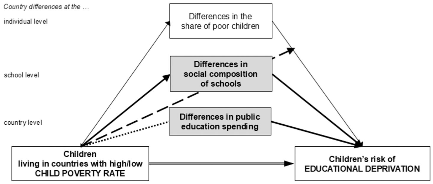
Conceptual framework summarizing the study’s research hypotheses on the relationship between child poverty rates and educational deprivation.

As a starting point, we hypothesize that national child poverty rates are positively associated with children’s risk of educational deprivation, even after accounting for cross-country differences in individual-level poverty risk factors (Hypothesis 1).

Second, we expect that lower public education spending partially explains the positive relationship between child poverty rates and educational deprivation (Hypothesis 2). We do not assert a causal relationship between child poverty rates and public education spending, but a correlation (as indicated by the dotted line in Figure 1; in our country sample: −0.479**, see Online Supplement, Table A2). One possible explanation is that weaker economic conditions increase child poverty and limit public resources, thus resulting in reduced social transfers (see definition of child poverty rates in the “Introduction” section) and lower public education spending (Busemeyer, 2007; Thévenon et al., 2018).⁶ To address this issue of potential confounding, we use spending as a percentage of GDP (like Ansell, 2008: 298) and control for GDP. Consistent with prior literature, we do, however, assume a directional effect from public education spending on educational outcomes, that is, lower public education spending is expected to increase the likelihood of educational deprivation (West and Nikolai, 2013).

Hypothesis 3 posits that part of the positive relationship between child poverty rates and educational deprivation is explained by country differences in school social composition. By definition, countries with higher child poverty rates have more disadvantaged (poor) students to distribute across schools, and—as already early addressed in the Coleman Report (Coleman et al., 1966) and supported by causal studies (e.g. Rumberger and Palardy, 2005)—a more disadvantaged social composition of schools tends to lower students’ academic achievement. However, whether school social composition in high-poverty countries affects all children or mainly those from disadvantaged families depends on how the “additional” poor children are distributed across schools (as indicated by the dashed arrow in Figure 1).

Figure 2 contrasts two different distribution scenarios. The “additional” poor students can be spread relatively proportionally across all schools (“proportional disadvantage” scenario), or they can be concentrated in a “few” high-poverty schools (“stronger concentration” scenario). To illustrate the difference between the two, consider two countries: country A has a child poverty rate of 10%, while country B’s rate is twice as high (20%). The PISA studies have shown that school segregation (between-school differences in their social composition) exists to some extent in all countries. Therefore, we posit some degree of school segregation in country A, with higher shares of poor children in schools in quintiles Q3–Q5. The left panel in Figure 2 assumes that country B’s “additional” 10 percentage points (pps) of poor children are distributed in such a way that schools in every quintile receive a higher proportion of poor children than in country A. Consequently, students in all quintiles in country B are more likely to have poor classmates than their counterparts in country A. Thus, both poor and non-poor students face a higher risk of educational deprivation in country B than in country A—that is why we call it the “proportional disadvantage” scenario.

Figure 2.

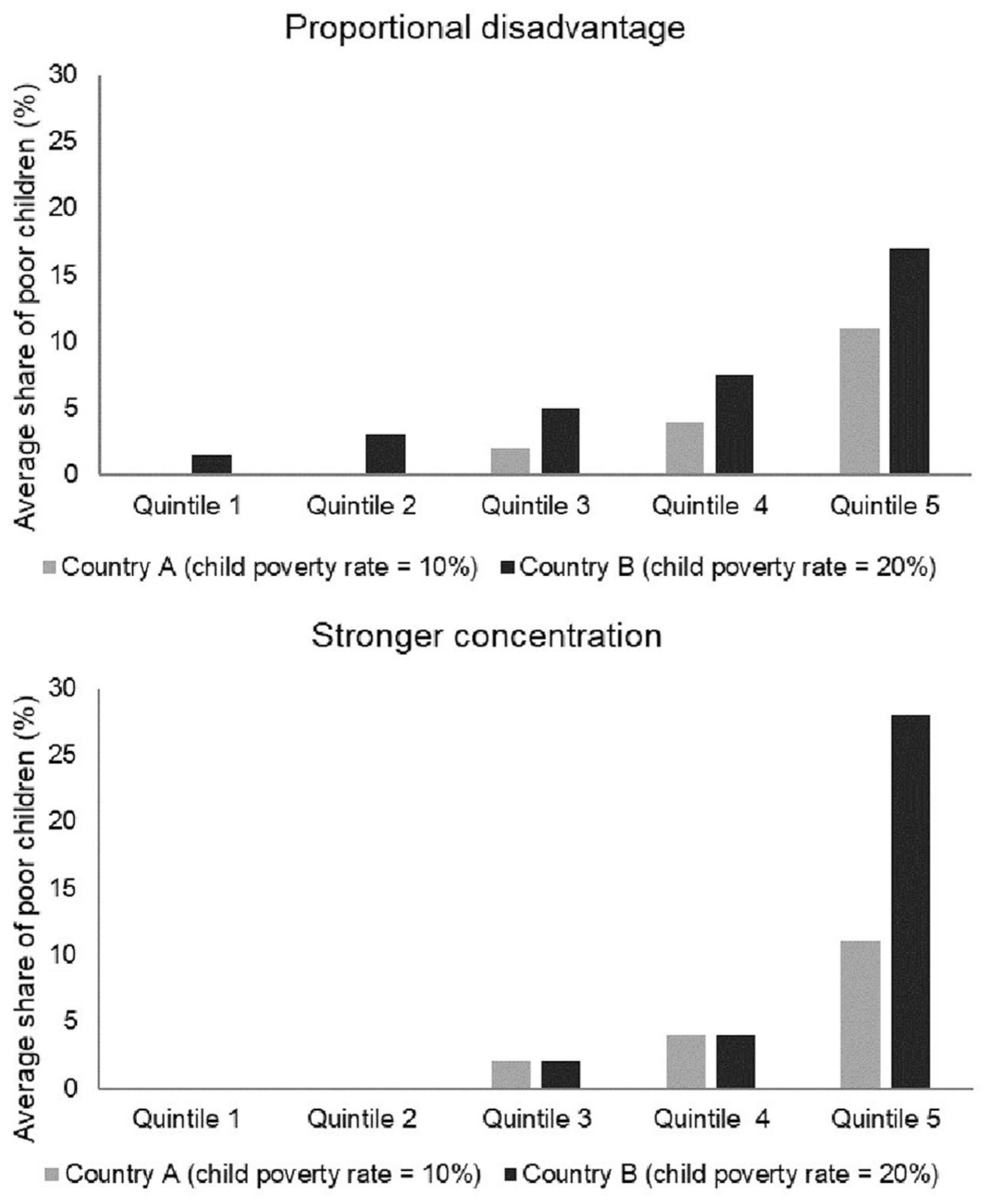
Stylized scenarios of differences in school social composition between countries with low and high child poverty rates.

The right panel in Figure 2 illustrates the alternative “stronger concentration” scenario. Here, the “additional” poor children in country B are distributed disproportionately across schools, with an even higher proportion of disadvantaged children in the poorest schools (quintiles Q4 and Q5). In this scenario, only poor children in country B are at a higher risk for educational deprivation than those in country A, while the risk for non-poor students (concentrated in quintiles Q1–Q3) remains almost the same. One reason to expect this pattern rather than “proportional disadvantage” is that social sorting between schools could be exacerbated if country B has external differentiation in secondary education (such as tracking between schools, as in Germany), or strong residential segregation (as in the US) (Borgna et al., 2019; Holtmann, 2016). Workman (2022) implicitly assumes that “stronger concentration” explains the positive association between regional income inequality and academic achievement in the US (without empirically testing it).

In sum, both distribution patterns are linked to higher overall levels of educational deprivation in country B, but they differ in whom they affect. The “stronger concentration” pattern mainly harms poor students, while the “proportional disadvantage” pattern increases the risk across all students. If high-poverty countries exhibit different distributional patterns (some proportional and some concentration), these opposing effects could cancel each other out in the analysis.

In the PISA data, students are nested within schools. Thus, we operationalize school social composition as the percentage of students from precarious households (see the “Data and methods” section). School composition effects may partly reflect neighborhood influences, particularly in countries with high residential segregation, such as the US (Burgess and Briggs, 2010). In less segregated contexts, such as Germany, schools in the same neighborhood can differ markedly in their social composition due to institutional tracking (i.e. due to sorting into different secondary school types) (Chmielewski, 2014). Regarding Hypothesis 3, the reason for school segregation—whether due to formal tracking or residential segregation—is less important. What matters is the extent to which students from different social backgrounds attend different schools.

Data and methods

Data and sample

To answer our research questions, we analyze PISA 2018 data from 32 countries.⁷ PISA assesses the competences of 15-year-old students in reading, mathematics, and science, providing internationally standardized test scores. Information about individual, family, and school background is collected via questionnaires from students and school officials. PISA samples are drawn using a two-stage stratified sampling procedure—first schools, then students. After excluding cases with missing information on the variables of interest (see below), our analysis sample comprises 228,874 students nested in 10,027 schools in 32 countries.

We use pre-pandemic PISA data (2018) rather than the most recent PISA 2022 wave. The COVID-19 pandemic generated large cross-national differences in school closures, remote learning, and home schooling. Consequently, PISA 2022 is not suitable for evaluating the school social composition mechanism, which rests on the assumption that child poverty rates are associated with differences in the learning and teaching environment within schools.

While Condron et al. (2024) pool data from several PISA waves, we decide against this longitudinal approach because, in our context, it would raise several methodological issues while adding little, given the limited over-time variation. First, since PISA scores are not vertically scaled, longitudinal analyses risk conflating substantive change with scale drift or framework differences, even when employing fixed-effects models (Contini and Cugnata, 2020). Second, the over-time variation in child poverty rates in our time frame is rather small. Using all pre-pandemic PISA waves from 2000 to 2018, our country panel dataset would cover the student assessments in the period from 1999 to 2017. A variance decomposition analysis of child poverty rates for our 32 countries over this period (345 country-years; data source: OECD.Stat) reveals that within-country variance is only 2.3% (corresponding to 8% of the overall variance), while the between-country variance is preponderant at 26.1% (corresponding to 92% of the overall variance).

Variables

Our dependent variable is children’s risk of educational deprivation. For our main analysis, we define educational deprivation as students scoring below PISA-defined proficiency level 2 (cut-off scores: 420 for math, 407 for reading, 410 for science; see Table 1). Since mathematics is more responsive to environmental influences than reading (see “Previous research” section), we use math as the primary educational outcome and reading and science for sensitivity checks. In additional analyses, we used students scoring below proficiency level 1 (cut-off scores: math 358, reading 335, science 335) as a measure of extreme educational poverty (see “Sensitivity analyses” section).

Table 1.

Descriptive statistics of country-level variables, sorted by child poverty rate.

Country	Child poverty rate	Public education spending	GDP per capita	Extent of educational deprivation: % children scoring below proficiency level 2
Country	(%)	(% of GDP)	(US$)	Mathematics	Reading	Science
Finland	3.6	3.59	47,570	13.3	12.8	11.9
Denmark	4.7	3.73	55,356	13.1	15.1	17.6
Slovenia	6.4	2.90	36,518	14.8	17.2	13.8
Czech Republic	6.8	2.44	38,843	19.2	20.1	18.0
Poland	6.8	2.77	29,609	12.5	13.6	12.6
Norway	8.0	4.66	64,589	17.7	18.5	20.1
Ireland	8.6	2.23	78,252	14.2	10.8	16.5
Sweden	9.3	3.86	51,948	17.6	17.8	18.1
Estonia	9.8	2.76	33,868	8.4	10.4	7.5
Hungary	9.9	2.61	29,496	24.6	25.1	23.9
Netherlands	9.9	3.03	55,090	14.8	23.5	19.7
Latvia	11.1	2.77	28,690	15.4	21.7	17.0
France	11.2	3.39	44,445	20.3	20.2	19.9
Germany	11.3	2.60	53,071	19.8	20.1	19.2
Canada	11.4	3.26	48,317	14.1	13.0	12.2
Austria	11.5	2.94	54,188	20.8	23.4	21.5
Slovak Republic	11.8	2.46	30,147	24.2	30.9	28.7
Switzerland	12.0	3.16	68,194	16.0	23.0	20.0
Portugal	12.2	3.55	33,045	22.5	19.5	18.6
Australia	12.5	3.23	50,759	21.5	19.1	18.3
United Kingdom	12.9	3.62	46,061	18.2	16.5	16.6
Luxembourg	13.9	2.54	114,863	26.9	28.7	26.4
Croatia	14.2	2.46	27,232	29.7	20.8	24.3
South Korea	14.2	3.03	40,957	13.7	14.3	13.6
Greece	15.9	2.56	28,605	34.5	29.8	31.3
New Zealand	17.6	3.19	41,994	20.4	18.4	17.6
Lithuania	18.4	2.26	33,762	24.5	24.0	21.3
Italy	18.7	2.77	41,951	23.2	22.3	25.2
Spain	19.6	2.63	39,601	23.1	–-	20.1
Bulgaria	20.2	1.79	21,458	44.8	47.1	46.8
United States	21.2	3.25	60,002	26.4	18.4	17.5
Romania	24.7	1.62	26,938	47.2	40.4	44.2
Mean	12.5	2.9	45,482	21.2	20.5	20.6
Standard deviation	4.9	0.6	18,184	8.5	8.5	8.1

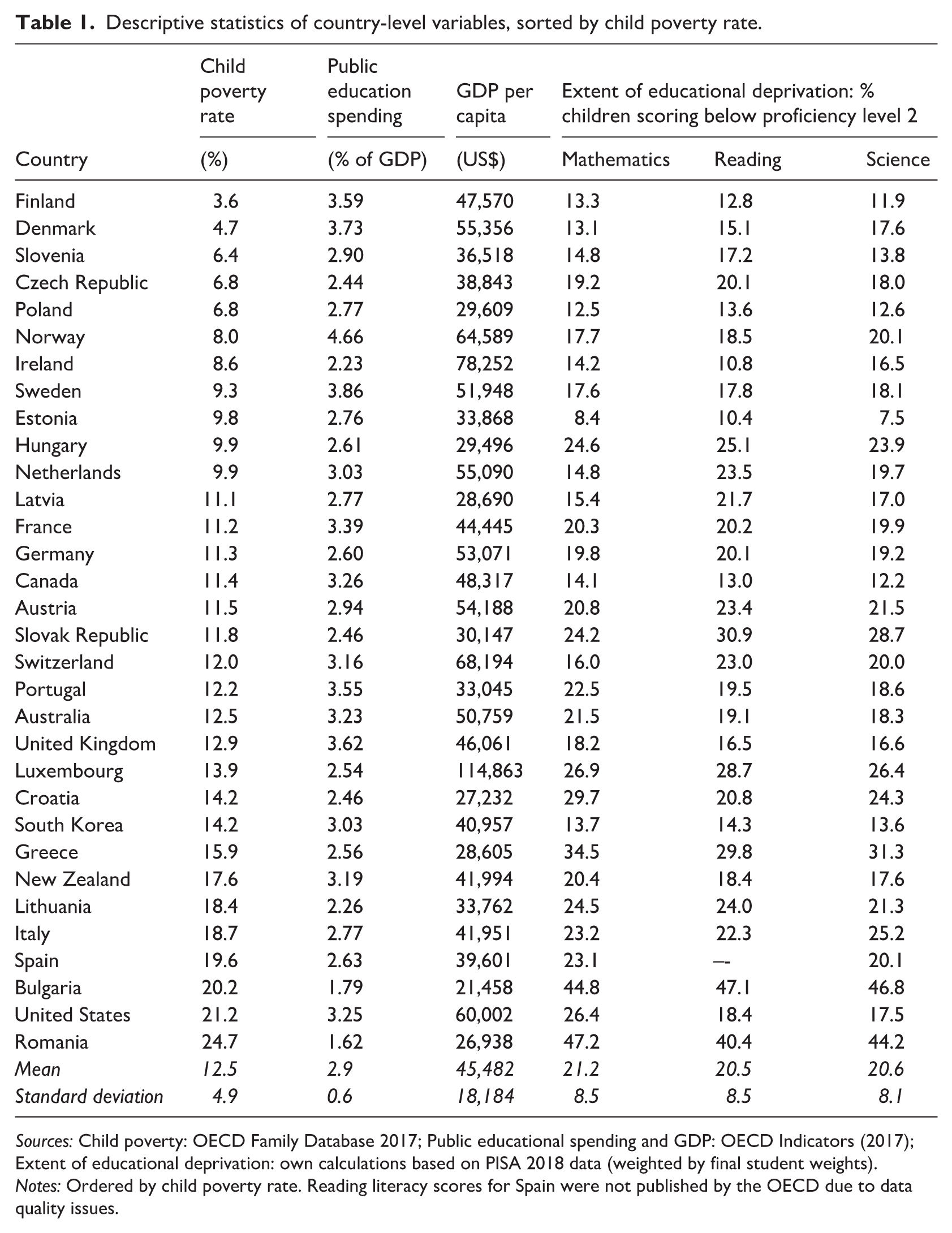
Sources: Child poverty: OECD Family Database 2017; Public educational spending and GDP: OECD Indicators (2017); Extent of educational deprivation: own calculations based on PISA 2018 data (weighted by final student weights).

Notes: Ordered by child poverty rate. Reading literacy scores for Spain were not published by the OECD due to data quality issues.

Our main country-level independent variable is the relative child poverty rate, measured as the percentage of individuals aged 0–17 living in households with an equivalized disposable income below 50% of the national median (the OECD poverty threshold). Relative income poverty indicates an income deemed insufficient for a decent standard of living in a given society, thereby placing individuals at risk of social exclusion. It captures poor children’s relative disadvantage in economic resources relevant to wellbeing and high educational achievement. We acknowledge that relative income poverty is only one facet of economic hardship, distinct from the other dimensions related to material deprivation and subjective financial stress (Schenck-Fontaine and Panico, 2019). Nevertheless, it is well-suited to this study’s objective and is the only measure readily available for comparing poverty across countries. Child poverty statistics are drawn from the OECD Family Database and refer to 2017, 1 year prior to the PISA assessment to ensure temporal precedence of the predictor (see Table 1). In the analyses, the variable is z-standardized (mean = 0, standard deviation (SD) = 1).

Ideally, given our focus, our analyses would have used child poverty rates for school‑aged children. These rates are unavailable, partly due to differences in the definition of “school age” across countries (e.g. differences in school starting ages and compulsory-education ages). We therefore conducted a sensitivity analysis using the country‑level share of 15-year-old students living in precarious households, estimated on the 2018 PISA sample, as a proxy for child poverty rates of school-aged children (see “Sensitivity analysis” section). The correlation between this share and the national child poverty rate is 0.675 (p < 0.01; see Online Supplement, Table A2).

To test Hypothesis 1—that the relationship between national child poverty and educational deprivation is not merely due to between-country differences in individual-level poverty risk (i.e. compositional differences)—we use the following individual-level variables:

- Precarious household conditions (categorical): very high precariousness = no employed parent; high precariousness = one parent not employed and the other in a low-skilled job (ISCO 9), both parents in low-skilled jobs, or one parent only: employed in a low-skilled job; reference category = at least one parent employed in a skilled job (ISCO 1–8).⁸

- Sometimes as a combined precariousness dummy variable: 1 = very high or high precariousness; 0 = having at least one parent employed in a skilled job (ISCO 1–8).

Because PISA lacks information on household income and because the validity and consistency of its home possession index has been questioned (Banerjee and Eryilmaz, 2024), we use parental employment status as a proxy for household economic conditions. Studies have shown that parental non-employment is the most important household-level determinant of child poverty (Thévenon et al., 2018: 30). In addition, employment in low-skilled jobs is a strong predictor of household poverty risk (Barbieri et al., 2024). Admittedly, ours is a rather conservative measure of precariousness—some families at risk of poverty are not classified as “poor” by our definition.

In all analyses, we include the precarious household conditions variable, as well as the following individual-level variables as controls: parental education (low = both parents without upper secondary education; medium = at least one parent with upper secondary education but neither with tertiary education; reference category, high = at least one parent with tertiary education), immigrant background (second-generation immigrant; first-generation immigrant; reference = otherwise, called “native”), and gender (female; reference = male).

To test Hypothesis 2, we use countries’ public education spending in 2017 as a percentage of GDP (again, measured 1 year prior to PISA 2018 to ensure temporal precedence). This includes spending on primary through post-secondary non-tertiary education (ISCED levels 1–4).⁹ Spending relative to GDP is a more comparable indicator than absolute spending because teacher salaries are a significant factor in spending and vary across countries (OECD, 2025). We also control for GDP per capita in 2017 to account for the fact that relative child poverty implies different levels of absolute deprivation in high- versus low-GDP contexts. Furthermore, higher GDP per capita is associated with higher per‑capita social expenditure, which may mitigate the effects of child poverty (Thévenon et al., 2018: 41). Descriptive statistics for both variables (drawn from OECD-Stat) are reported in Table 1.

Testing Hypothesis 3 requires operationalizing the school-level share of children at risk of poverty. We use two school-level variables computed from the PISA 2018 data:

- School share of students from precarious households: aggregation of the individual-level precariousness dummy variable at the school level (see above), z-standardized across countries to facilitate interpretation of the coefficients.

- Top‑quintile (Q5) school dummy variable: a binary indicator equal to 1 if the school is in the country’s 20% of schools with the highest share of students from precarious households (Q5), and 0 otherwise (Q1–Q4).

In additional analyses, we operationalize the school share of students from precarious households as a categorical variable with four levels: 0–4%, 4–7%, 7–12%, and over 12% (see “Sensitivity analyses” section). These cut-offs are based on the empirical distribution of the indicator: 4% is the average, 7% is the 75th percentile, and 12% is the 90% percentile.

Analytical strategy

To account for PISA’s two-stage sampling procedure, we estimate three-level mixed-effects linear probability models¹⁰ on the probability of being in educational deprivation as follows

Y_{i j k} = α_{0} + β_{k} X_{i j k} + γ W_{j k} + μ Z_{k} + u_{j k} + u_{k} + ε_{i j k}

where Y_ijk represents the probability of educational deprivation (defined as scoring below proficiency level 2 in the main analysis) in a given PISA competence domain; X_ijk is a vector of individual-level factors, which we allow to have different effects across countries (random slopes β_k); W_jk is a vector of school-level factors; Z_k is a vector of country-level factors; and u_jk and u_k are the random intercepts at the school and country level, respectively. The models were estimated in STATA 18 without sampling weights because weighted models failed to converge.¹¹ Our inferential goal is to estimate model-based conditional associations between student outcomes and covariates, rather than obtaining design-based descriptive population parameters. Prior research using PISA and similar large-scale assessments shows that unweighted multilevel models may affect variance component estimates but have negligible impact on fixed-effect coefficients, which are the focus of this study (Rutkowski et al., 2010). Moreover, when models include variables closely related to the sampling design (e.g. student and school characteristics), unweighted model-based inference remains consistent and interpretable (Gelman, 2007). Descriptive statistics and population-level summaries reported in the paper are weighted using final student weights.

We test our hypotheses by estimating a sequence of models. The null model (M0) and a model with only the individual-level variables (M1) show whether there is variance to be explained at the school and country levels. For Hypothesis 1, we estimate two models: M2a, which only includes the national child poverty rate and controls for GDP (M2a), and M2b, which adds individual-level precariousness and socio-demographic controls (see above). By comparing the child poverty rate coefficients in M2a and M2b, we assess whether cross-country compositional differences explain the correlation between child poverty and educational deprivation.

To test Hypothesis 2, we estimate a model that adds public education spending (M3a). We compare the child poverty rate coefficients in M3a and M2b to assess how much of the child poverty effect is explained by education spending. Model M3b includes random slopes for the individual-level controls, allowing their coefficients to vary across countries. Because random slopes demand more statistical power, we dichotomize the categorical individual-level control variables. Since M3a and M3b produce similar results, we use dummy control variables with random slopes in all subsequent models.

For Hypothesis 3, we estimate two models: M4a adds the school-level share of students from precarious households, while M4b further adds the top‑quintile (Q5) school dummy variable. Comparing the child poverty coefficient in M3b with those in M4a and M4b reveals the extent to which school social composition explains the observed association between child poverty rates and educational deprivation.

To investigate the nature of school social composition in high child poverty contexts (i.e. whether the “additional” poor students are concentrated or proportionally distributed across schools), we estimate two models: M5a includes the cross-level interaction between national child poverty and individual-level household precariousness, but it omits the school-level composition variables. If the “stronger concentration” pattern is predominant (i.e. national poverty mainly affects poor children), we expect a positive cross-level interaction and a near-zero baseline coefficient for national child poverty. In contrast, if the “proportional disadvantage” pattern predominates (i.e. also non-poor students are affected), we expect a positive baseline estimate for national child poverty, indicating in this model the educational deprivation risk for non-poor children in high-poverty countries (reference category). Model M5b adds the school-level variables to M5a. In a “stronger concentration” scenario, we should also observe a decline in the interaction coefficient when school social composition is included (M5b), suggesting that school segregation mediates the interaction effect. To complement our multivariate models, we also descriptively explore how students from economically precarious families are distributed across the different country-specific quintiles of household precariousness in schools, as well as how the shares of educationally deprived students from precarious and non-precarious households vary by national poverty rates. By doing so, we can explore whether high-poverty countries exhibit similar or different patterns in the distribution of additional poor students across schools.

Results

Child poverty is prevalent among the study’s high-income countries and, as shown in Figure 3, it positively correlates with educational deprivation (r = 0.675, p < 0.01, see Table A2, Online Supplement, for the other literacy domains).

Figure 3.

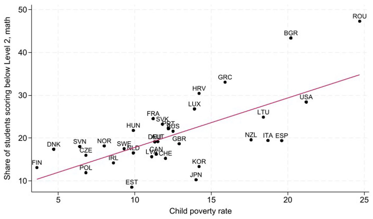
Scatterplot of educational deprivation by child poverty rate, at the country level.

Model M2a in Table 2 confirms this substantial association: a 1SD increase in the child poverty rate is associated with a 5.4 pp rise in educational deprivation—implying a 10.8 pp difference between low- and high-poverty countries. Comparing the intra-class correlation (ICC) of models M0 and M2a reveals that the unexplained variance at the country level is substantially reduced (from 5.1% to 2.8%) once child poverty rate enters as predictor.

Table 2.

Three-level mixed-effects linear probability models of educational deprivation (defined as scoring below math proficiency level 2).

	M0	M1	M2a	M2b	M3a	M3b	M4a	M4b	M5a	M5b
Individual-level variables
Precarious households (HH) (Ref.: at least one parent in skilled job)
a: Both parents employed in low-skilled jobs (ISCO 9), or one employed in a low-skilled job and the other not employed, or one parent only: employed in a low-skilled job		0.105**		0.105**	0.105**
b: No parent is employed		0.152**		0.152**	0.152**
Precarious HH dummy (a + b) (Ref.: at least one parent in skilled job)						0.120**	0.096**	0.096**	0.119**	0.095**
Parental education (Ref.: high)
Medium		0.107**		0.107**	0.107**
Low		0.019**		0.019**	0.019**
Low parental education dummy (Ref.: high or medium)						0.113**	0.106**	0.107**	0.113**	0.107**
Migration status (Ref.: native)
a: Second-generation immigrant		0.058**		0.058**	0.058**
b: First-generation immigrant		0.087**		0.087**	0.087**
Migration status dummy (a + b) (Ref.: native)						0.079**	0.077**	0.076**	0.079**	0.076**
Gender: Girls (Ref.: boys)		0.018**		0.018**	0.018**	0.020**	0.020**	0.021**	0.020**	0.021**
School-level variables
% of students from precarious HH at school (z-std.)							0.071**	0.059**		0.059**
School in Q5 (highest % of students from precarious HH) (Ref: schools in Q1-Q4)								0.045**		0.045**
Country-level variables
Child poverty rate (z-std.)			0.054**	0.049**	0.038**	0.040**	0.027*	0.029**	0.040**	0.029**
Public education spending as % of GDP (z-std.)					−0.023⁺	−0.019	−0.016	−0.016	−0.019	-0.016
GDP (z-std.)			−0.022⁺	−0.027*	−0.022⁺	−0.022*	−0.018⁺	−0.019⁺	−0.022*	-0.019 +
Cross-level interaction
Precarious HH dummy x child poverty (z-std.)									0.013⁺	0.014 +
Intra-class correlation
Country-level	0.051	0.050	0.028	0.028	0.026	0.021	0.019	0.019	0.022	0.019
School-level	0.254	0.234	0.236	0.216	0.215	0.211	0.172	0.172	0.211	0.172

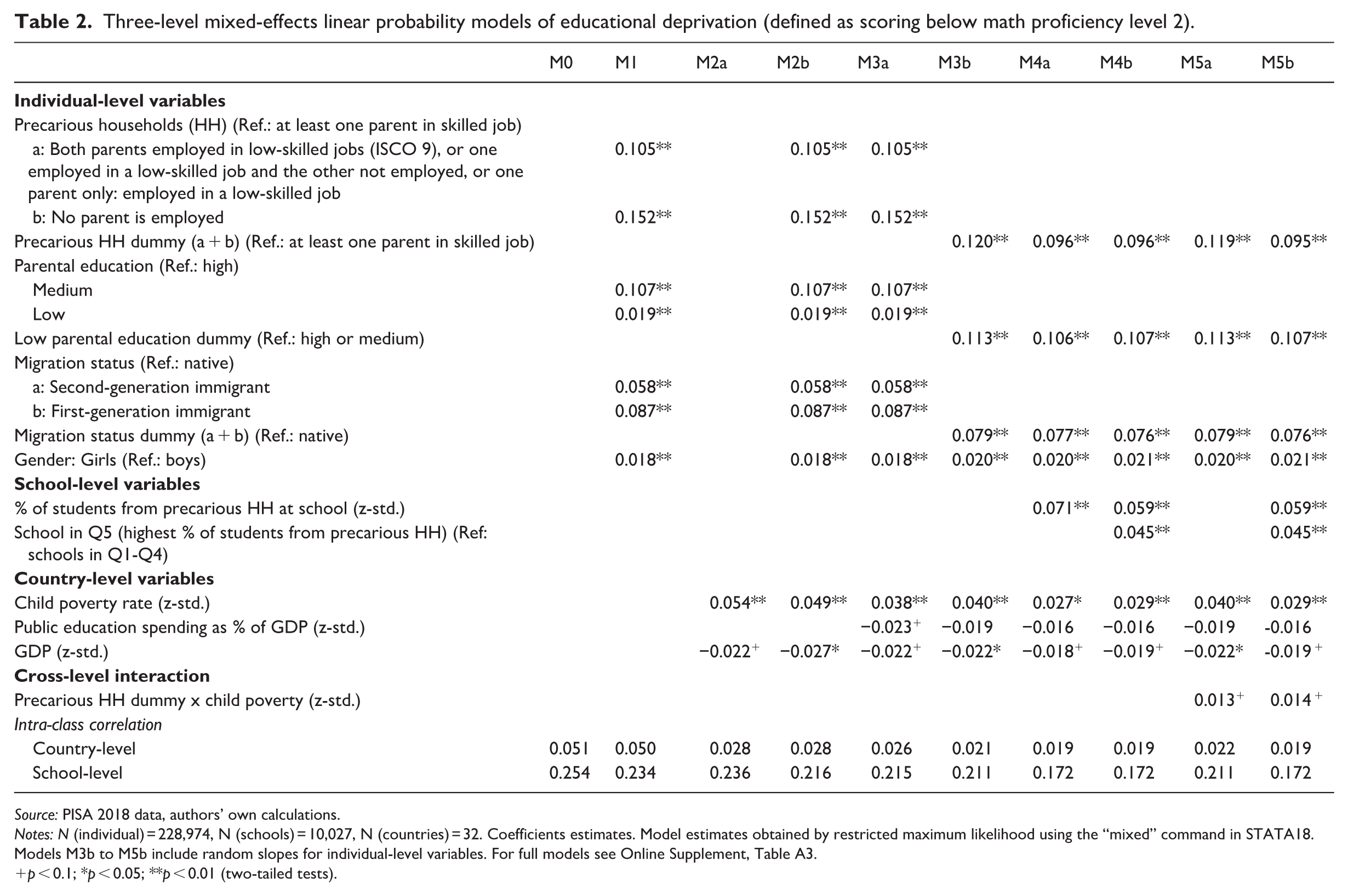
Source: PISA 2018 data, authors’ own calculations.

Notes: N (individual) = 228,974, N (schools) = 10,027, N (countries) = 32. Coefficients estimates. Model estimates obtained by restricted maximum likelihood using the “mixed” command in STATA18. Models M3b to M5b include random slopes for individual-level variables. For full models see Online Supplement, Table A3.

+p < 0.1; *p < 0.05; **p < 0.01 (two-tailed tests).

We now examine our three hypotheses concerning the factors that explain this relationship. Model M2b tests Hypothesis 1 by accounting for cross-country compositional differences. M2b shows that precarious household conditions and low parental education are strongly associated with a higher risk of educational deprivation. While the child poverty rate coefficient is reduced compared with M2a, it remains substantial at 4.9 pp (corresponding to a 9.8 pp difference between low- and high-poverty countries). This indicates that national child poverty rates exert an effect beyond compositional differences, supporting Hypothesis 1.

As expected, public education spending is negatively correlated with the child poverty rate (r = -0.479, p < 0.01; see Online Supplement, Table A2). Models M3a and M3b test Hypothesis 2. In both models, higher public education spending is associated with a lower risk of educational deprivation (about 2 pp for a 1-SD increase). However, the estimate only reaches the 10% significance level in M3a, and is not significant in M3b, which includes random slopes for the individual-level covariates. Accordingly, the unexplained variance at the country level is only marginally reduced (from 28% to 26%). The formal model comparison confirms a modest improvement of model fit once educational spending is included (see Online Supplement, Table A4). Importantly for our hypothesis, adding public education spending reduces the estimated effect of national child poverty from 4.9 pp (M2b) to 3.8 pp in M3a and 4 pp in M3b, consistent with Hypothesis 2.

Models M4a and M4b begin testing Hypothesis 3, which states that differences in school social composition partially mediate the child poverty-educational deprivation association. Consistent with this hypothesis, the child poverty coefficient in M4a is notably smaller than in M3a and M3b. In line with US findings (Workman, 2022), our findings are consistent with the interpretation that school social composition is a key mediating mechanism through which higher child poverty rates increase the risk of educational deprivation.¹² It is also worth noting that the two school composition coefficients are positive and statistically significant, even when estimated jointly (M4b): A 1-SD increase in the share of students from precarious households raises children’s risk of educational deprivation by about 6 pp (equivalent to a 12 pp difference between schools with low vs high shares of precarious families). In addition, attending a school in the poorest national quintile (Q5) increases the risk by 4.5 pp relative to students attending schools in quintiles Q1–Q4. Including variables accounting for school social composition differences significantly reduces the unexplained variance at both the country level (from 2.6% to 1.9%) and the school level (from 21.0% to 17.2%; see also the formal model comparison in Online Supplement, Table A4).

To explore the nature of school social composition related to our two scenarios for the distribution of “additional” poor children across schools, we estimated M5a and M5b. Both models include a cross-level interaction between national child poverty rates and the individual-level household precariousness: M5a includes only this interaction, while M5b additionally includes the school-level variables. The interaction coefficients are positive but small and reach only marginal significance (p < 0.10); correspondingly, including the cross-level interactions does not improve model fit (see Online Supplement, Table A4). In M5a, the interaction suggests that, compared with low-poverty countries, children from precarious households in high-poverty countries are about 2.6 pp (−1 SD vs +1 SD) more likely to experience educational deprivation than their non-precarious counterparts. Furthermore, the child poverty coefficient indicates that children from non-precarious families are 8 pp more likely to experience educational deprivation in high-poverty countries than in low-poverty countries. When school composition is included (M5b), the interaction coefficient remains unchanged, but the child poverty coefficient declines substantially.

Figure 4 graphically displays the predicted probabilities for the estimated interactions between precarious household conditions and national child poverty rates of M5a and M5b. The figure shows that as national child poverty increases, children’ risk of educational deprivation increases for both “poor” and “non-poor” students in a similar way, as evidenced by the rather parallel trends. In addition, we see that school social composition partially explains these higher risks, as the predicted probabilities are lower in M5b than in M5a. These estimates are consistent with the descriptive findings shown in Table 3 that the share of educationally deprived students is higher in countries with greater child poverty, not only among children from precarious households (correlation r = 0.503, p < 0.001), but also, markedly, among children from non-precarious households (correlation r = 0.709, p < 0.001).

Figure 4.

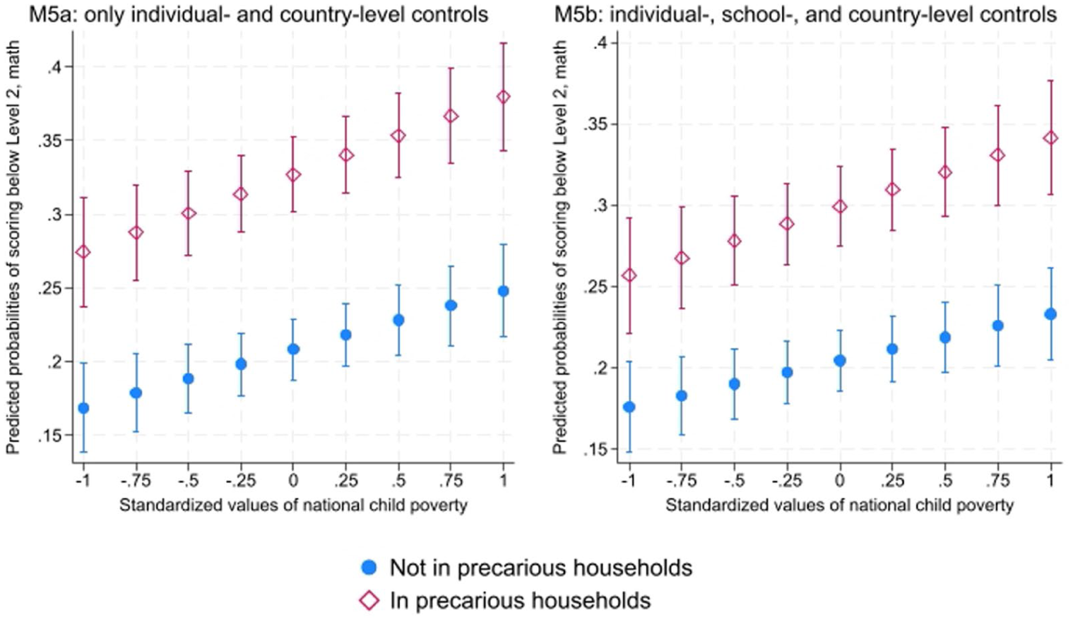
Predicted probabilities of educational deprivation by precarious household conditions (dummy variable) and national child poverty rates.

Table 3.

Quintiles’ average shares of students from economically precarious families in school and educational deprivation by family background (in %).

Country	Child poverty rate	Quintiles’ average share of students					% of educationally deprived
		from precarious households in schools					students from
		Q1	Q2	Q3	Q4	Q5	precarious HH	non-precarious HH
Finland	3.6	0.0	0.0	0.0	3.5	6.9	34.8	11.1
Denmark	4.7	0.0	0.0	3.2	4.4	11.0	35.0	11.5
Slovenia	6.4	0.0	0.0	0.0	3.7	10.5	31.7	13.5
Czech Rep.	6.8	0.0	0.0	0.0	3.7	11.6	51.4	17.3
Poland	6.8	0.0	0.0	0.0	3.5	8.5	25.5	10.9
Norway	8.0	0.0	0.0	0.0	4.1	8.6	40.6	15.6
Ireland	8.6	0.0	0.0	2.7	3.9	8.8	31.0	12.3
Sweden	9.3	0.0	0.0	0.0	3.6	9.9	39.7	14.2
Estonia	9.8	0.0	0.0	0.0	3.0	10.9	22.8	7.1
Hungary	9.9	0.0	0.0	0.0	3.7	18.9	68.6	21.0
Netherlands	9.9	0.0	0.0	2.7	3.9	9.8	27.8	12.1
Latvia	11.1	0.0	0.0	0.0	5.1	14.8	30.0	12.3
France	11.2	0.0	3.1	3.5	7.3	19.4	46.0	16.4
Germany	11.3	0.0	0.0	3.6	4.5	13.3	46.9	15.7
Canada	11.4	0.0	2.6	3.2	5.4	14.3	28.4	11.6
Austria	11.5	0.0	0.0	3.1	4.7	14.2	47.8	17.2
Slovakia	11.8	0.0	0.0	0.0	3.8	18.8	59.8	19.8
Switzerland	12.0	0.0	0.0	3.2	5.2	11.8	37.8	13.0
Portugal	12.2	0.0	0.0	3.7	6.8	17.2	53.7	19.4
Australia	12.5	0.0	0.0	0.0	5.2	13.7	41.0	19.4
United Kingdom	12.9	0.0	0.0	3.3	5.2	13.3	39.3	15.2
Luxembourg	13.9	0.6	2.2	3.8	6.5	10.7	50.6	24.0
Japan	14.0	0.0	0.0	2.9	3.2	6.4	0.2	0.1
Croatia	14.2	0.0	2.4	2.6	4.3	8.6	57.3	27.8
South Korea	14.2	0.0	2.6	2.8	6.3	12.4	25.5	12.1
Greece	15.9	0.0	3.0	4.0	7.2	17.2	55.4	31.3
New Zealand	17.6	0.0	1.4	2.5	5.3	12.3	50.2	17.6
Lithuania	18.4	0.0	0.0	3.3	4.7	16.1	51.2	20.7
Italy	18.7	0.0	3.4	4.2	7.2	19.4	46.7	20.3
Spain	19.6	0.0	3.0	6.0	9.3	16.1	42.5	20.4
Bulgaria	20.2	0.0	0.0	3.6	8.4	30.9	69.8	37.4
US	21.2	0.0	2.8	3.5	6.4	13.5	46.4	23.2
Romania	24.7	0.4	3.1	6.7	14.5	30.3	77.8	42.3
Corr. with child poverty rate		0.297⁺	0.601 **	0.705 **	0.760 **	0.643 **	0.503 **	0.709 **

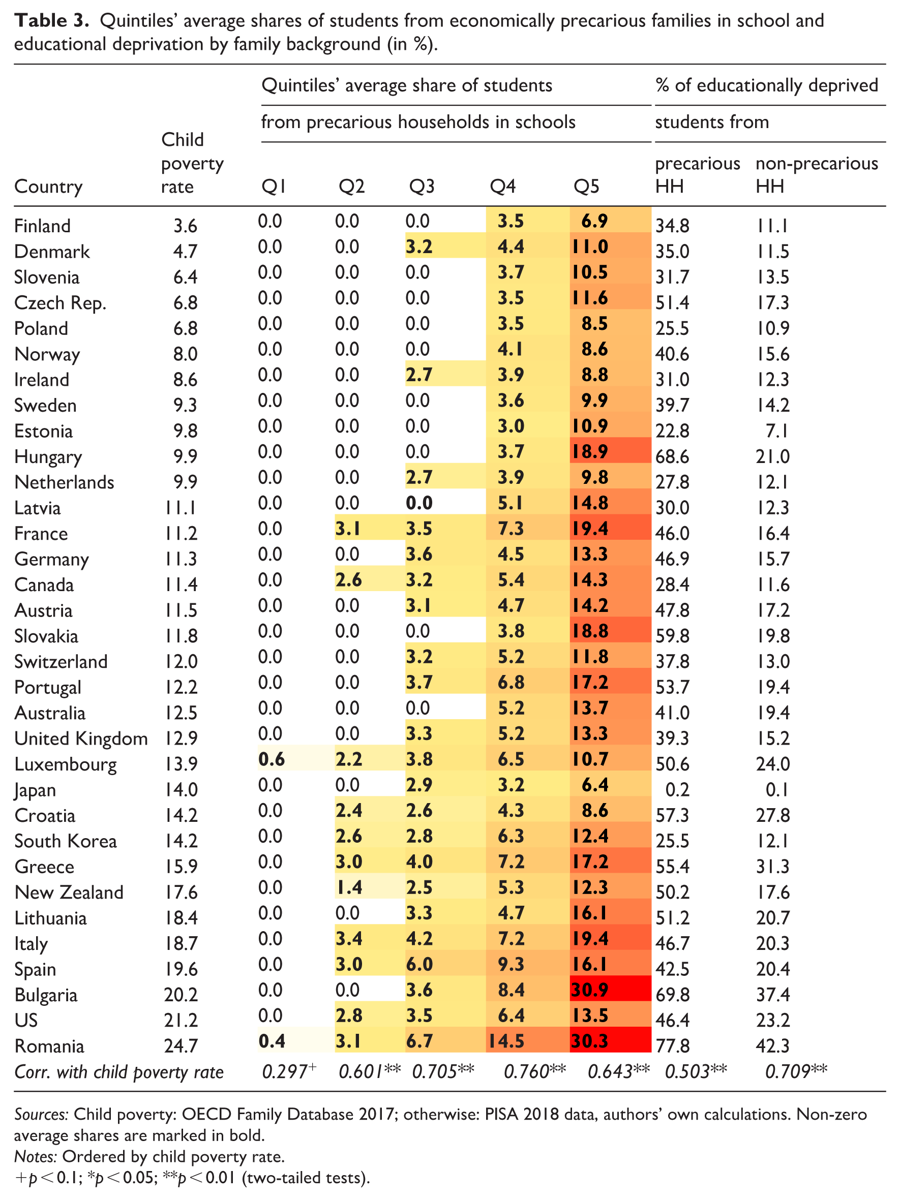
Sources: Child poverty: OECD Family Database 2017; otherwise: PISA 2018 data, authors’ own calculations. Non-zero average shares are marked in bold.

Notes: Ordered by child poverty rate.

p < 0.1; *p < 0.05; **p < 0.01 (two-tailed tests).

Together, these findings indicate that high levels of national child poverty affect not only children from precarious households but also have spillover effects on children from non-precarious households through exposure to disadvantaged peers. This suggests that “proportional disadvantage” is the predominant pattern in high-poverty countries rather than “stronger concentration.”

Table 3 supports this conclusion. It presents a heat map of the average share of children from precarious households by school quintile for each country, displaying descriptively how the “additional” poor children are distributed across schools in higher-poverty countries. The map reveals that a high concentration of disadvantaged students in high-poverty schools (Q5) is not confined to high-poverty countries. In fact, in most low-poverty countries (below 10% child poverty), poor children are almost exclusively concentrated in low-poverty schools (Q4 and Q5). By contrast, in most high-poverty countries (above 15%), poor children are distributed across nearly all quintiles, except Q1. Countries with mean child poverty rates (10–15%) occupy an intermediate position: poor children are mostly found in medium- to high-poverty schools (Q3–Q5), that is, in 60% of schools. These distributional patterns are more consistent with the “proportional disadvantage” than with the “stronger concentration” scenario.

Sensitivity analyses

The results presented so far concern mathematical literacy. Previous research finds that math is more sensitive to income inequality than reading (see “Previous research” section). One explanation is that reading competences are largely shaped at a very early age, while math competences are more responsive to environmental factors, including schooling, at later ages (Farkas and Beron, 2004; Little et al., 2021; Lonigan et al., 2000). Workman (2022) suggests a further explanation: in high-inequality regions/countries, high-SES parents intensify the support of their children’s academic development, particularly in reading—potentially offsetting for them the negative effects of national income inequality on reading achievement. This interpretation is in line with Condron et al.’s (2024) findings that national child poverty reduces the share of high-achieving students in math but not in other subjects.

To explore domain differences, we rerun our model sequence for reading and science (see Online Supplement, Tables A6 and A7). Model M2a shows that the child poverty effect is slightly weaker for reading and science than for math: the difference between high- and low-poverty countries in educational deprivation is 8.8 (= 2*4.4) pp in reading and 8.4 pp in science, compared with 10.8 pp in math. Crucially, the overall pattern of results is consistent across the three domains: adding individual-level controls (M2b) reduces, but does not eliminate, the child poverty effect (supporting Hypothesis 1); adding public education spending (M3a) further reduces the child poverty effect (supporting Hypothesis 2); and adding school-level social composition variables (M4a/M4b) decreases the child poverty effect further (supporting Hypothesis 3).

Thus far, we have defined educational deprivation as scoring below PISA proficiency level 2. We also re-estimated all models using a more restrictive definition: scoring of below proficiency level 1 (extreme educational deprivation) (see Online Supplement, Tables A8 to A10). The results using this definition largely support the three hypotheses. The coefficients for national child poverty are smaller than in the level 2 specification, likely because, by definition, the prevalence of scoring below level 1 is lower (as is also reflected by the intercept estimates).

Furthermore, we address the potential nonlinearity of the school composition variable by re-estimating model M4a using four categories for the share of students from precarious households (for the definition see “Data and methods” section). The results indicate that very low shares of poor students (up to 4%) are not associated with increased risks of educational deprivation, while medium shares of 4–7% and 7–12% lead to increases of about 5.5 pp and 4.8 pp, respectively. High shares (above 12%) are associated with the greatest increase (14.4 pp). Thus, while a high concentration of poor students in school is particularly harmful, the effects of social school composition are already visible—and substantially almost linear—at lower levels of concentration. Since the reduction in the child poverty rate estimate is the same when including this categorical variable as when including the school composition variables of the main analysis, this again strengthens our conclusion that it “proportional disadvantage” rather than “stronger concentration” is the main explanation.

To address potential measurement error of our national child poverty indicator, which covers all children aged 0–17 rather than only school children (see “Data and methods” section), we reran all our analyses using the share of 15-year-old students from precarious households, as estimated from the 2018 PISA sample, as the main country-level predictor. These results largely confirm those of our main models (see Online Supplement, Table A12).

Finally, to rule out the possibility that our results are driven by single outlier countries, we re-estimated our main models M3b and M4b excluding one country at a time. The results proved to be highly stable to this inclusion/exclusion exercise (see Online Supplement, Figures A1 and A2).

Discussion and conclusion

Comparative research on cross-national differences in educational achievement and inequality has traditionally focused on education system characteristics. Recently, scholars have begun examining how broader societal conditions—such as income inequality at the national or regional level—relate to levels and social disparities in educational outcomes (see Borgna et al., 2019, for a review). Our study contributes to this literature on the social embeddedness of schooling and education by investigating whether national child poverty rates influence children’s risk of experiencing educational deprivation in advanced economies, using PISA 2018 data. Societal child poverty is one of the non-school factors that has received relatively little attention (see Hannum and Xie, 2017, for a review). To date, only the country-level study by Condron et al. (2024) has explicitly examined the role of national child poverty, providing compelling evidence that it affects academic achievement. Building on their findings, our study aims to unpack two possible mechanisms underlying this relationship: the patterns of school social composition in contexts of high child poverty and public education spending.

Our analyses reveal a positive and substantial association between national child poverty rates and children’s risk of educational deprivation. This association only modestly decreases when accounting for individual-level measures of parental precariousness, indicating that societal child poverty independently shapes educational outcomes. Our study provides evidence that lower public education spending is associated with higher educational deprivation and reduces the positive correlation between the national child poverty rate and educational deprivation. This suggests that high-poverty countries do not compensate for their children’s higher risk of low educational achievement. On the contrary, they tend to allocate fewer resources to schools.

Furthermore, our analyses show that accounting for the share of students from economically precarious households in schools (a proxy for concentration of poverty at the school level) substantially reduces the effect size of the national child poverty rate. Hence, school social composition explains a substantial part of the association between child poverty and educational deprivation, resonating with findings from the US (Workman, 2022). Importantly, the mediating role of school social composition persists net of public education spending. To our knowledge, this is the first cross-national study to test for spending and school segregation simultaneously.

Our study also contributes to a better understanding of the nature of school segregation in societal contexts of high(er) child poverty. Our analyses provide fairly compelling evidence that societal child poverty harms both poor and non-poor children because the “additional” poor children are spread across schools—challenging the assumption that higher child poverty necessarily produces intensified segregation (Workman, 2022). Our results suggest that, at least within our country sample, the “additional” poor children of high-poverty countries are dispersed across schools, following a “proportional disadvantage” pattern. This leads to spillover effects of disadvantageous school environments to non-poor children.

In sum, our study identifies two pathways through which societal child poverty translates into educational inequality by linking a macro indicator (national child poverty) to both a macro-level (public education spending) and a meso‑level (school social composition) mechanism, which together shape individual outcomes (i.e. children’s risk of educational deprivation). This advances theories of stratification and segregation by demonstrating that national economic conditions influence the social organization of schools, thereby structuring peer environments, resource distribution, and children’s educational opportunities.

Our findings have clear policy implications. First, they underscore the substantial societal costs of child poverty. Poverty at any level—individual, school, and national—elevates children’s risk of educational deprivation. Second, although public education spending could in principle mitigate these harms, high-poverty countries are currently not compensating for them through school funding, as they tend to invest less in education, not more.

Third, financial resources alone are not enough; interventions that address school social composition and segregation are also required. Countries with high societal child poverty rates have more schools that are challenged by the impoverished situation of poor children, producing spillovers that also harm their non-poor schoolmates. Thus, reducing educational deprivation requires both targeted compensatory funding (i.e. increased public education spending focused on schools with a high concentration of poor students) and measures to reduce school segregation, such as housing policies that reduce residential segregation and institutional de-tracking reforms in order to limit early sorting. Finally, and importantly, our results underscore the social embeddedness of schooling. Schools alone cannot reduce educational deprivation in countries with a high proportion of children living in poverty. Therefore, addressing child poverty directly by increasing families’ economic resources and improving parents’ labor market opportunities is also essential (Solga, 2014).

Although our study is comprehensive in terms of competence domains and levels of educational deprivation, several limitations suggest fruitful directions for future research. First, its cross-sectional design precludes establishing causal relationships. Future work could exploit longitudinal data, policy reforms, or quasi-experimental designs to identify causal effects. Second, PISA does not provide information on household income or direct measures of child poverty at the individual or school level, so we had to rely on proxies for poverty risk, such as parental employment precariousness. Where possible, linking PISA to administrative income records or using survey data with direct household income would reduce measurement error and concerns about omitted variables. Third, our analysis of public education spending does not capture inequities in the allocation of resources across schools within countries—a critical issue highlighted by UNICEF (2023). This is challenging to address in cross-nationally comparative research due to data limitations (Chmielewski and Bell, 2024). Consequently, we are likely to underestimate the importance of targeted public education spending. Fourth, even after accounting for spending and school social composition, the child poverty coefficient remains statistically significant and substantively meaningful in our full models. This indicates that further mechanisms are likely involved. Future research should investigate additional pathways. Despite these limitations, our study complements the findings by Condron et al. (2024) by elucidating plausible meso- and macro-level mechanisms linking national child poverty to educational deprivation.

Supplemental Material

sj-docx-1-cos-10.1177_00207152261454241 – Supplemental material for Unpacking the relationship between child poverty rates and educational deprivation: The role of school social composition and public education spending

Supplemental material, sj-docx-1-cos-10.1177_00207152261454241 for Unpacking the relationship between child poverty rates and educational deprivation: The role of school social composition and public education spending by Camilla Borgna, Martina Dieckhoff and Heike Solga in International Journal of Comparative Sociology

Footnotes

Acknowledgements

We thank the editor and reviewers of the journal, as well as the participants of the AAM/HIS/NEPS Colloquium at the WZB—Berlin Social Science Center, of the ESPAnet 2025 Conference in Milan of the German Sociological Association Conference 2025 in Duisburg and of the 2026 RC28 Spring Meeting in Sevilla for their valuable feedback.

ORCID iDs

Camilla Borgna

Martina Dieckhoff

Funding

The authors received no financial support for the research, authorship, and/or publication of this article.

Declaration of conflicting interests

The authors declared no potential conflicts of interest with respect to the research, authorship, and/or publication of this article.

Supplemental material

Supplemental material for this article is available online.

Notes

References

Agasisti

Longobardi

Prete

, et al. (2021) The relevance of educational poverty in Europe: Determinants and remedies. Journal of Policy Modeling 43(3): 692–709.

Allmendinger

Leibfried

(2003) Education and the welfare state. Journal of European Social Policy 13(1): 63–81.

Ansell

(2008) Traders, teachers, and tyrants: Democracy, globalization, and public investment in education. International Organization 62(2): 289–322.

Banerjee

Eryilmaz

(2024) A critical evaluation of the validity of socioeconomic measures used in PISA. International Journal of Comparative Education and Development 26(4): 342–375.

Barbieri

Cutuli

Scherer

(2024) In-work poverty in Western Europe. European Societies 26(4): 1232–1264.

Bischoff

Owens

(2019) The segregation of opportunity: Social and financial resources in the educational contexts of lower- and higher-income children, 1990–2014. Demography 56: 1635–1664.

Bodovski

Byun

S-Y

Chykina

, et al. (2017) Searching for the golden model of education: Cross-national analysis of math achievement. Compare 47(5): 722–741.

Borgen

(2024) It’s not all about the peers: Reintroducing school context to the school segregation literature. Acta Sociologica 67(1): 66–87.

Borgna

Brzinsky-Fay

Dieckhoff

, et al. (2019) Beyond schools: The social embeddedness of educational inequality. In: Becker

(ed.) Research Handbook on the Sociology of Education. Edward Elgar, pp.575–589.

10.

Burgess

Briggs

(2010) School assignment, school choice and social mobility. Economics of Education Review 29(4): 639–649.

11.

Busemeyer

(2007) Determinants of public education spending in 21 OECD democracies, 1980–2001. Journal of European Public Policy 14(4): 582–610.

12.

Carbonaro

Lauen

Levy

(2023) Does cumulative exposure to high-poverty schools widen test-score inequality? Sociology of Education 96(2): 81–103.

13.

Checchi

Van de Werfhorst

Braga

, et al. (2014) The policy response to educational inequalities. In: Salverda

Nolan

Checchi

, et al. (eds) Changing Inequalities in Rich Countries. Oxford University Press, pp.294–327.

14.

Chmielewski

(2014) An international comparison of achievement inequality in within- and between-school tracking systems. American Journal of Education 120: 293–324.

15.

Chmielewski

(2019) The Global Increase in the Socioeconomic Achievement Gap, 1964 to 2015. American Sociological Review 84(3): 517–544.

16.

Chmielewski

Bell

(2024) Cross-national socioeconomic inequality and educational policy. In: Berends

Schneider

Lamb

(eds) The Sage Handbook of Sociology of Education. Sage, pp.327–342.

17.

Chzhen

Howarth

Main

(2021) Deprivation and intra-family conflict. Journal of Marriage and Family 84: 121–140.

18.

Coleman

Campbell

Hobson

, et al. (1966) Equality of Educational Opportunity. U.S. Department of Health, Education, and Welfare, Office of Education.

19.

Condron

(2011) Egalitarianism and educational excellence. Educational Researcher 40(2): 47–55.

20.

Condron

Roscigno

(2003) Disparities within: Unequal spending and achievement in an urban school district. Sociology of Education 76(1): 18–36.

21.

Condron

Merry

Samard

, et al. (2024) Child poverty and academic skills at the national level: A longitudinal analysis of four waves of PISA. International Journal of Comparative Sociology 66(6): 849–868.

22.

Contini

Cugnata

(2020) Does early tracking affect learning inequalities? Revisiting difference-in-differences modeling strategies with international assessments. Large-scale Assessments in Education 8(1): 14.

23.

Daniele

(2021) Socioeconomic inequality and regional disparities in educational achievement: The role of relative poverty. Intelligence 84: 101515.

24.

Duncan

Yeung

Brooks-Gunn

, et al. (1998) How much does childhood poverty affect the life chances of children? American Sociological Review 63(3): 406–423.

25.

Engle

Black

(2008) The effect of poverty on child development and educational outcomes. Annals of the New York Academy of Sciences 1136: 243–256.

26.

Epple

Romano

(1996) Ends against the middle: Determining public service provision when there are private alternatives. Journal of Public Economics 62(3): 297–325.

27.

Farkas

Beron

(2004) The detailed age trajectory of oral vocabulary knowledge: Differences by class and race. Social Science Research 33: 464–497.

28.

Finch

Hernández Finch

(2022) The relationship of national, school, and student socioeconomic status with academic achievement. Frontiers in Education 7: 857451.

29.

Gelman

(2007) Struggles with survey weighting and regression modeling. Statistical Science 22(2): 153–164.

30.

Giddens

(1998) The Third Way: The Renewal of Social Democracy. Polity Press.

31.

Goldin

Katz

(1997) Why the United States led in education. NBER Working Paper no. w6144. NBER.

32.

Granvik Saminathen

Brolin Låftman

Almquist

, et al. (2018) Effective schools, school segregation, and the link with school achievement. School Effectiveness and School Improvement 29(3): 464–484.

33.

Hannum

Xie

(2017) Education. In: Brady

Burton

(eds) Oxford Handbook of the Social Sciences of Poverty. Oxford University Press, pp.462–485.

34.

Hermann

Kisfalusi

(2026) School segregation, student achievement, and educational attainment in Hungary. International Journal of Comparative Sociology 67(1): 69–94.

35.

Holtmann

(2016) Excellence through equality of opportunity. In: Blossfeld

Buchholz

Skopek

, et al. (eds) Models of Secondary Education and Social Inequality. Edward Elgar, pp.61–76.

36.

Holzberger

Reinhold

Lüdtke

, et al. (2020) A meta-analysis on the relationship between school characteristics and student outcomes in science and math. Studies in Science Education 56(1): 1–34.

37.

Justice

Jiang

Purtell

, et al. (2019) Conditions of poverty, parent–child interactions, and toddlers’ early language skills in low-income families. Maternal and Child Health Journal 23: 971–978.

38.

Karagiannaki

(2017) The empirical relationship between income poverty and income inequality in rich and middle-income countries. CASE Paper 206. Center for Analysis of Social Exclusion.

39.

Langenkamp

Carbonaro

(2018) How school socioeconomic status affects achievement growth across school transitions in early educational careers. Sociology of Education 91(4): 358–378.

40.

Little

Lonigan

Phillips

(2021) Differential patterns of growth in reading and math skills during elementary school. Journal of Educational Psychology 113(3): 462–476.

41.

Lonigan

Burgess

Anthony

(2000) Development of emergent literacy and early reading skills in preschool children. Developmental Psychology 36: 596–613.

42.

McLoyd

Jocson

Williams

(2017) Linking poverty and children’s development. In: Brady

Burton

(eds) Oxford Handbook of the Social Sciences of Poverty. Oxford University Press, pp.141–167.

43.

Merry

(2013) Tracing the U.S. deficit in PISA reading skills to early childhood. Sociology of Education 86: 234–252.

44.

Merry

Condron

Torres

(2021) A comparative analysis of early childhood socioeconomic conditions and educational achievement 15 years later. International Journal of Comparative Sociology 61(6): 389–411.

45.

Murnane

(2007) Improving the education of children living in poverty. Future Child 7: 161–182.

46.

Musterd

(2005) Social and ethnic segregation in Europe: Levels, causes, and effects. Journal of Urban Affairs 27: 331–348.

47.

Nieuwenhuis

Kleinepier

Van Ham

(2021) The role of exposure to neighborhood and school poverty in understanding educational attainment. Journal of Youth and Adolescence 50: 872–892.

48.

Nikolai

(2011) Towards social investment? Patterns of public policy in the OECD world. In: Morel

Palier

Palme

(eds) Towards a Social Investment Welfare State? Bristol University Press, pp.91–116.

49.

OECD (2016) Low-Performing Students: Why they Fall Behind and How to Help Them Succeed. OECD Publishing.

50.

OECD (2019) PISA 2018 Assessment and Analytical Framework. OECD Publishing.

51.

OECD (2024) Child Poverty CO2.2. OECD Family Database. Available at: https://webfs.oecd.org/els-com/Family_Database/CO_2_2_Child_Poverty.pdf (accessed 4 April 2025).

52.

OECD (2025) How Are countries balancing teaching staff compensation with broader education investment? Education Indicators in Focus no. 89. OECD Publishing.

53.

Orfield

Lee

(2005) Why Segregation Matters: Poverty and Educational Inequality. The Civil Rights Project, UCLA. Available at: https://escholarship.org/uc/item/4xr8z4wb (accessed 26 December 2024).

54.

Owens

(2018) Income segregation between school districts and inequality in students’ achievement. Sociology of Education 91(1): 1–27.

55.

Pit-ten Cate

Kroezen

Ottenbacher

, et al. (2026) The long-term impact of socioeconomic school composition on inequalities in track placement and student achievement growth in Luxembourg. International Journal of Comparative Sociology 67(1): 137–174.

56.

Ponnet

(2014) Financial stress, parent functioning and adolescent problem behavior. Journal of Youth and Adolescence 43: 1752–1769.

57.

Rauscher

Mellon

Hodgman

(2025) School spending and student achievement: Mechanisms. Policy Insights from the Behavioral and Brain Sciences 12(2): 171–176.

58.

Reardon

Weathers

Fahle

, et al. (2024) Is separate still unequal? New evidence on school segregation and racial academic achievement gaps. American Sociological Review 89(6): 971–1010.

59.

Rumberger

Palardy

(2005) Does segregation still matter? Teachers College Record 107(9): 1999–2045.

60.

Rutkowski

Gonzalez

Joncas

, et al. (2010) International large-scale assessment data: Issues in secondary analysis and reporting. Educational Researcher 39(2): 142–151.

61.

Schenck-Fontaine

Panico

(2019) Many kinds of poverty: Three dimensions of economic hardship, their combinations, and children’s behavior problems. Demography 56(6): 2279–2305.

62.

Schoon

Hope

Ross

, et al. (2010) Family hardship and children’s development. Longitudinal and Life Course Studies 1: 209–222.

63.

Sen

(1990) Development as capability expansion. In: Griffin

Knight

(eds) Human Development and the International Development Strategy for the 1990S. Palgrave Macmillan, pp.41–58.

64.

Sen

(1999) Commodities and Capabilities. Oxford University Press.

65.

Shanks

(2007) The impacts of household wealth on child development. Journal of Poverty 11(2): 93–116.

66.

Shavit

Park

(2016) Introduction to the special issue: Education as a positional good. Research in Social Stratification and Mobility 43(1): 1–5.

67.

Sirin

(2005) Socioeconomic status and academic achievement: A meta-analytic review of research. Review of Educational Research 75(3): 417–453.

68.

Solga

(2014) Education, economic inequality, and the promises of the social investment state. Socio-economic Review 12(2): 269–297.

69.

Thévenon

Manfredi

Govind

, et al. (2018) Child poverty in the OECD: Trends, determinants and policies to tackle it. OECD Social, Employment and Migration Working Papers, no. 218. OECD Publishing.

70.

Thorson

Gearhart

(2018) The adverse effects of economic inequality on educational outcomes: An examination of PISA scores, 2000–2015. World Affairs 181: 286–306.

71.

Tucker-Drob

Cheung

Briley

(2014) Gross domestic product, science interest, and science achievement. Psychological Science 25(11): 2047–2057.

72.

UNICEF (2023) Transforming Education with Equitable Financing. UNICEF.

73.

West

Nikolai

(2013) Welfare regimes and education regimes: Equality of opportunity and expenditure in the EU (and US). Journal of Social Policy 42(3): 469–493.

74.

Wodtke

Harding

Elwert

(2011) Neighborhood effects in temporal perspective. American Sociological Review 76(5): 713–736.

75.

Workman

(2022) Inequality begets inequality: Income inequality and socioeconomic achievement gradients across the United States. Social Science Research 107: 102744.

76.

Workman

(2023) Income inequality and student achievement: Trends among US States (1992–2019). Educational Review 75(5): 871–893.

Supplementary Material

Please find the following supplemental material available below.

For Open Access articles published under a Creative Commons License, all supplemental material carries the same license as the article it is associated with.

For non-Open Access articles published, all supplemental material carries a non-exclusive license, and permission requests for re-use of supplemental material or any part of supplemental material shall be sent directly to the copyright owner as specified in the copyright notice associated with the article.

0.00 MB

0.22 MB