Circuit analysis using the node-impedance method

Abstract

Circuit analysis is essential for studying other more specialized areas of electrical engineering. Traditional tools of analysis include the mesh current method and the node voltage method; however, neither approach is universally applicable to all circuit configurations. In this work, we introduce the node-impedance method as a comprehensive framework for electric circuit analysis. This method serves as an effective alternative to classical techniques and, in many practical situations, offers a more straightforward implementation. The node-impedance method is applicable to all types of circuits without additional steps. By knowing in advance the transfer gain between nodes, the method facilitates the systematic construction of the signal-flow graph. The proposed method can be used to solve simple and complex circuits, calculate transfer functions, and solve feedback circuits containing one or more loops. From a pedagogical perspective, the node-impedance method is particularly valuable, as it provides insight into the circuit topology uncovers non-obvious interconnections between nodes, and reveals hidden feedback loops.

Keywords

circuit analysis driving-point impedance transfer function feedback undergraduate teaching

Introduction

Circuit analysis is a fundamental skill, learned by students in their first year of an Electrical Engineering program. Traditional tools of analysis include the mesh current method and the node voltage method. The mesh current method is best suited to circuits containing voltage sources, whereas nodal analysis is best suited to circuits excited by current sources. The modified nodal analysis (MNA) is an extension of nodal analysis, which not only solves for the node voltages but also uses some branch currents as the unknown parameters.¹ In principle, any circuit can be solved by using MNA. However, the resulting equations contain redundancy, making computer-based solution methods essential.

A number of studies used signal-flow graphs for circuit analysis. A flow graph is a directed graph in which nodes represent system variables, while the edges (or branches) represent the connections between nodes.² An algorithm, known as Mason's rule, is used for calculating the transfer gain between two nodes.³ It has been demonstrated that the topological structure of a flow graph depends only upon the algebraic structure of the set of equations.⁴ For an overview of signal flow analysis for feedback networks.⁵ A method that uses both current and voltage graphs for the symbolic analysis of circuits containing active elements has been presented.⁶ Circuits with feedback can be analyzed, first by taking small-signal Thevenin and Norton equivalent circuits to remove feedback, and then by constructing the circuit signal-flow graph.⁷ Thevenin and Norton equivalent circuits were utilized to model the loading effects of the feedback network before forming the signal-flow graph and solving the resulting circuit equations.^8,9

Some works rely on the concept of driving-point impedance (DPI) to analyze electrical networks. To determine the DPI at a given port, the port is excited with a 1-A AC current source, and the resulting voltage across the port terminals is measured. The DPI of a specific node can be defined by taking the reference node as ground. Both feedback and non-feedback circuits were analyzed by computing the DPI and then using the current-divider and the voltage-divider equations to calculate currents and voltages.⁹ The unknown potential of a node can be calculated by taking the product of the short-circuit current and the DPI of that node.¹⁰ A different application of the DPI concept was presented.¹¹ A cut is done close to the output node at a point in the external feedback path. Then two sources are applied: one driving the feedback network and the other driving the load and the amplifier output. One source is set to magnitude one and the other is zeroed. Then the excitation pattern is switched. This way four currents are generated, and from those the loop gain can be calculated. The method is suitable for circuits with bilateral feedback. Using the concept of DPI the circuit transposition theorem was proved using signal-flow graphs.¹² A form of graphs that are optimum for a quick “hand-and-paper” analysis of circuits containing ideal op amps was proposed.¹³

As mentioned earlier, traditional circuit analysis techniques rely on either mesh currents or nodal voltages as the primary variables, which makes them unsuitable for certain classes of circuits. Approaches based on signal-flow graphs use both voltage and current as variables; however, formulating the appropriate equations is not straightforward. Considerable experience is needed to construct a signal-flow graph that is manageable and efficient to analyze.

This paper introduces a new circuit analysis method founded on the concept of node impedance, which is fundamentally different from the DPI approach. The central objective is to establish a procedure that directly yields node transfer gains (transmission coefficients) in a clear and systematic way. Once derived, the resulting equations can be solved by hand for relatively simple circuits or by using computer power for more complex configurations.

Theoretical foundation of the method

The concept of node impedance

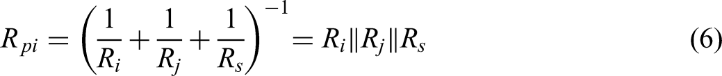
The concept of node impedance is central to the implementation of the node-impedance method. The node impedance is defined as the impedance “seen” at a specific node when all sources are turned off and all other nodes are connected to ground. It is important to note that the node impedance differs from the DPI of the same node measured with respect to ground. When measuring DPI, there is no requirement to connect all other nodes to ground and disable controlled sources. It will be demonstrated that the node impedance helps in determining the transfer gain between two nodes. As an example, consider the circuit shown in Fig. 1.

Figure 1.

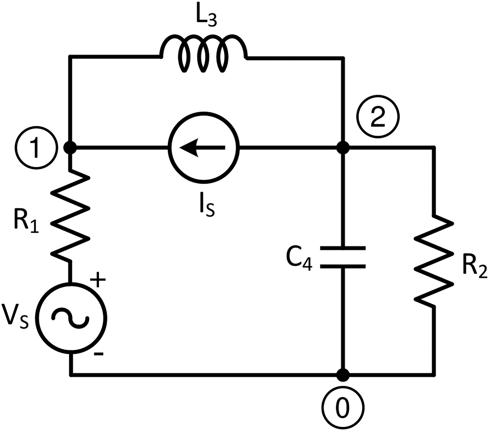
Circuit to demonstrate the concept of node impedance. The reference node is labeled 0.

According to the definition given in the previous paragraph the node impedances for nodes 1 and 2 are

Z_{p 1} = R_{1} ‖ j ω L_{3} Z_{p 2} = R_{2} ‖ j ω L_{3} ‖ \frac{1}{j ω C_{4}}

(1)

where the operator ‖ denotes the parallel combination of the impedances involved. The node impedance matrix is a diagonal matrix containing the impedances of all nodes. The node impedance matrix for the circuit of fig. 1 is as follows:

Z_{p} = [\begin{matrix} Z_{p 1} & 0 \\ 0 & Z_{p 2} \end{matrix}]

(2)

General expression for the transfer gain between two nodes

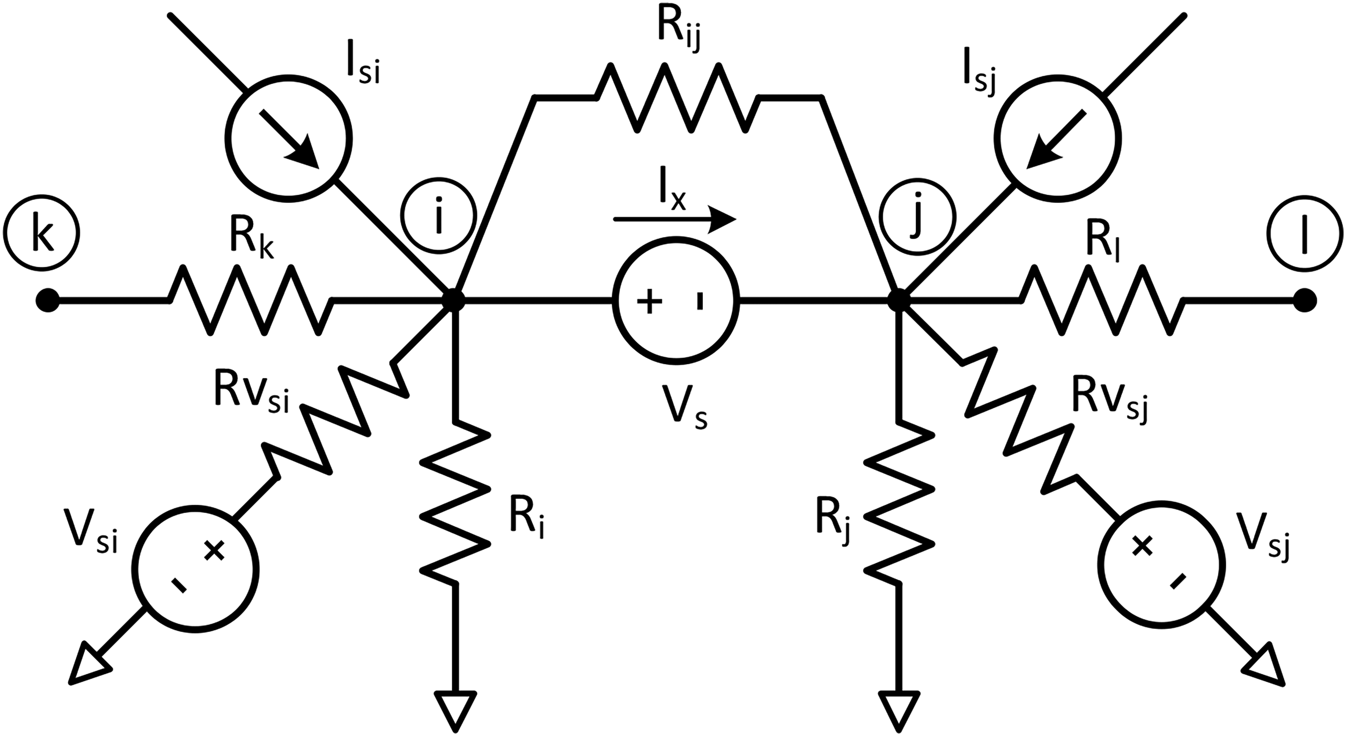
In this paragraph, the relation between the branch impedances and the transmission coefficient from one node to another will be established. Consider the following part of a circuit, depicting nodes i, j, associating elements R_i, R_j, R_s and sources I_s, V_s.

Kirchhoff's current law for node i is written as

Fig 2.

\frac{E_{i} - E_{j}}{R_{j}} + \frac{E_{i}}{R_{i}} + \frac{E_{i} - V_{s}}{R_{s}} - I_{s} = 0

(3)

Figure 2.

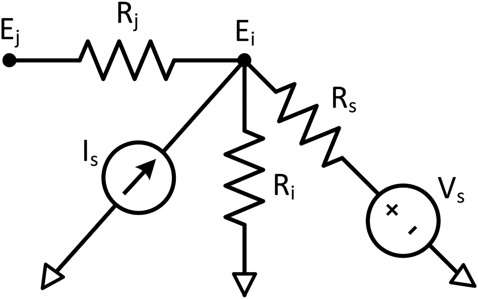
Circuit for the derivation of transfer-gain between nodes.

We may rewrite eqn (3) as

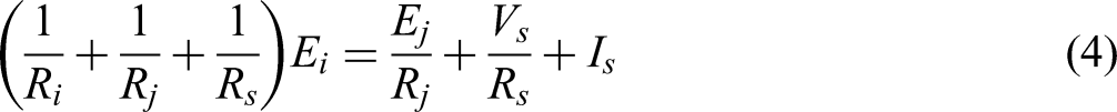
(\frac{1}{R_{i}} + \frac{1}{R_{j}} + \frac{1}{R_{s}}) E_{i} = \frac{E_{j}}{R_{j}} + \frac{V_{s}}{R_{s}} + I_{s}

(4)

Using the concept of node impedance, eqn (4) can be written in a more compact form as follows:

E_{i} = \frac{R_{p i}}{R_{j}} E_{j} + \frac{R_{p i}}{R_{s}} V_{s} + R_{p i} I_{s}

(5)

where the node impedance R_pi for node i is

R_{p i} = {(\frac{1}{R_{i}} + \frac{1}{R_{j}} + \frac{1}{R_{s}})}^{- 1} = R_{i} ‖ R_{j} ‖ R_{s}

(6)

that is the parallel combination of resistors R_i, R_j, R_s. From expression 5, we see that node j contributes a gain R_pi/R_j to node i, while voltage source V_s contributes a gain R_pi/R_s. In general, the gain from any other node to node i is the node impedance R_pi divided by the impedance connecting the two nodes (transfer impedance). For a current source I_s the gain is simply R_pi; thus, for current sources, the gain equals the node impedance. These rules apply for any node and also apply for controlled voltage and current sources. It should be obvious from the above analysis that an ideal voltage source with zero internal resistance accepts no return signals from adjacent nodes.

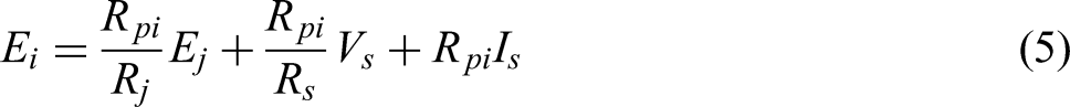
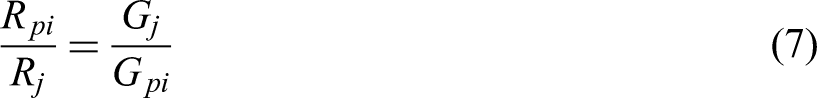
The resistances ratio R_pi/R_j can alternatively be written as a ratio of conductances.

\frac{R_{p i}}{R_{j}} = \frac{G_{j}}{G_{p i}}

(7)

where the node conductance is defined as

G_{p} = G_{i} + G_{j} + G_{s} = \frac{1}{R_{i}} + \frac{1}{R_{j}} + \frac{1}{R_{s}},

(8)

with all sources disabled and the other nodes connected to ground. In this work, we will use the form that employs resistances.

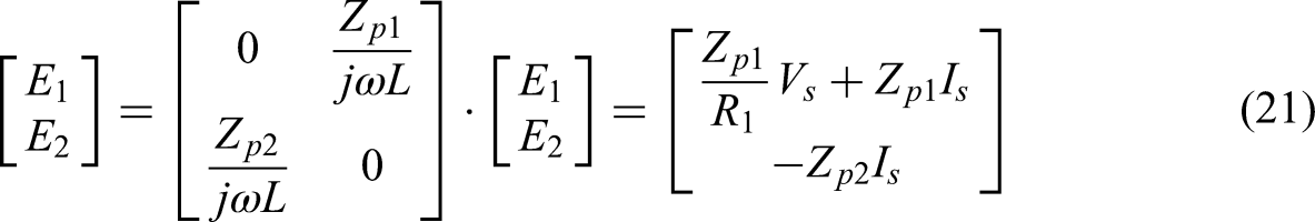
Relation between the node-impedance method and the node-voltage method

The node-voltage method is a well-established method. The equations are a generalization of the Ohm's law and the general form of them is

Y_{n} E = J_{s}

(9)

where Y_n is the node admittance matrix

E is the node voltages matrix

J_s is the node current source vector

The general form of the node-impedance equations is

E = T E + S

(10)

where T denotes the transmission coefficient matrix, also referred to as the transfer gain matrix

S denotes the sources matrix

The solution of eqns (10) is

E = (I - T)^{- 1} \cdot S

(11)

where I is the identity matrix of dimensions n x n. Equation (11) offers a general method for solving the node-impedance equations and it will be used extensively in the following sections.

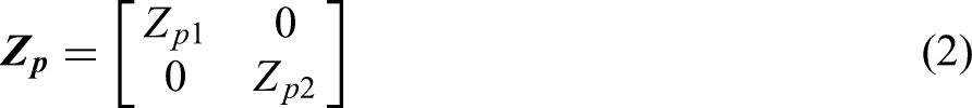
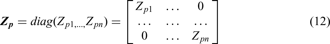
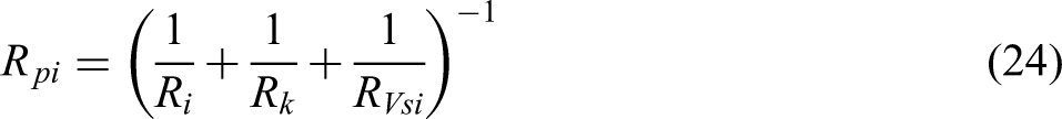
At this point, it is helpful to establish the relation between the node-voltage equations and the node-impedance equations. First, we introduce the node impedance matrix Z _p , defined as the diagonal matrix that contains all node impedances

Z_{p} = d i a g (Z_{p 1, \dots,} Z_{p n}) = [\begin{matrix} Z_{p 1} & \dots & 0 \\ \dots & \dots & \dots \\ 0 & \dots & Z_{p n} \end{matrix}]

(12)

It is easy to show that the following relation between S and J_s holds

S = Z_{p} J_{s}

(13)

Solve eqn (9) for E to get

E = Y_{n}^{- 1} J_{s}

(14)

Similarly, solve eqn (10) for E to get

E = (I - T)^{- 1} S

(15)

where I as usual is the identity matrix. Combining eqns (14) and (15) we get

Y_{n}^{- 1} J_{s} = (I - T)^{- 1} S

(16)

and substituting S from eqn (13)

Y_{n}^{- 1} J_{s} = (I - T)^{- 1} Z_{p} J_{s}

(17)

Equation (17) can be solved for the node admittance matrix.

Y_{n} = Z_{p}^{- 1} (I - T)

(18)

Therefore, the set of equations relating the node-voltage method to the node-impedance method is:

Y_{n} = Z_{p}^{- 1} (I - T) J_{s} = Z_{p}^{- 1} S

(19)

Alternatively, eqns (19) can be written in the form:

T = I - Z_{p} Y_{n} S = Z_{p} J_{s}

(20)

We conclude that the sets [ T , S ] and [ Y_n , J_s ] are connected through a linear transformation. In most practical cases, the equations relating T and S have a simpler form than those relating Y_n and J_s .

Solution of electric circuits with the node-impedance method

In this section, we will focus on the practical application of the method, presenting a series of examples that encompass a broad range of electrical circuits.

Circuits with independent voltage sources that have non-zero internal impedance

Consider again the circuit of Fig. 1 where R₁ = 5 Ω, R₂ = 8 Ω, L₃ = 6 H, C₄ = 0.25 F, V_s = 20cost, I_s = 0.5cos(t + 45^o). Based on the theoretical framework presented in the previous paragraph, the circuit's signal-flow graph can be directly constructed by inspection, as the transfer gain between nodes is known (Fig. 3).

Figure 3.

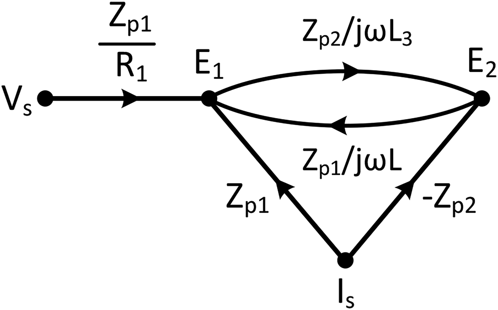
Signal-flow graph of the circuit of Fig. 1.

The node-impedance equations for the signal-flow graph of Fig. 3 in matrix form are

[\begin{matrix} E_{1} \\ E_{2} \end{matrix}] = [\begin{matrix} 0 & \frac{Z_{p 1}}{j ω L} \\ \frac{Z_{p 2}}{j ω L} & 0 \end{matrix}] \cdot [\begin{matrix} E_{1} \\ E_{2} \end{matrix}] = [\begin{matrix} \frac{Z_{p 1}}{R_{1}} V_{s} + Z_{p 1} I_{s} \\ - Z_{p 2} I_{s} \end{matrix}]

(21)

where the node impedances Z_p₁, Z_p₂ are taken from eqn (1). Substituting the values and solving the system using Eq. 11 we get

E_{1} = 9.758 ∠ {49.2}^{o} V E_{2} = 11.088 ∠ - {91.9}^{o} V

(22)

The time domain expressions for the voltages are e₁(t) = 9.758cos(t + 49.2^o), e₂(t) = 11.088cos(t–91.9^o).

Circuits that have an ideal voltage source floating between two nodes

When an ideal voltage source is present between two nodes, the gain from one node to the other becomes indeterminate because the source branch has zero impedance. To address this, one approach is to introduce a small fictitious branch resistance r, solve the circuit, and then take the limit as r → 0. Another way of getting around the problem is to use the source-shifting technique, where the ideal voltage source is transferred to all adjacent branches. If the branch receiving the shifted source has impedance, the gain is well-defined. If it contains a current source, the voltage source is effectively absorbed by the current source. Both methods are valid, but here we will demonstrate a way to handle the problem directly. Consider the following part of a circuit, where the ideal voltage source V_s is connected between nodes i and j, with several other elements connected to either node i or node j (Fig. 4).

Figure 4.

An ideal voltage source is connected between nodes i and j (floating voltage source).

Writing the equations for nodes i, j, summing them and solving for the potential E_i of node i we get

E_{i} = - \frac{R_{p i}}{R_{p j}} E_{j} + \frac{R_{p i}}{R_{k}} E_{k} + \frac{R_{p i}}{R_{l}} E_{l} + \frac{R_{p i}}{R_{V s i}} V_{s i} + \frac{R_{p i}}{R_{V s j}} V_{s j} + R_{p i} I_{s i} + R_{p i} I_{s j}

(23)

where the impedance of node i is

R_{p i} = {(\frac{1}{R_{i}} + \frac{1}{R_{k}} + \frac{1}{R_{V s i}})}^{- 1}

(24)

From eqn (23) we conclude that all nearby nodes and sources contribute some gain to node i. In addition, the ideal voltage source V_s imposes the limitation

E_{i} - E_{j} = V_{s} \to E_{j} = E_{i} - V_{s}

(25)

Elements that are common in nodes i and j, such as the resistance R_ij, do not appear in eqn (23) and hence they do not contribute to the gain. The circuit shown in Fig. 4 is fairly general; in specific applications, some components may be missing. The signal-flow graph is shown in Fig. 5. Most edges end up to node i. The gains for node j are either 1 or −1.

Figure 5.

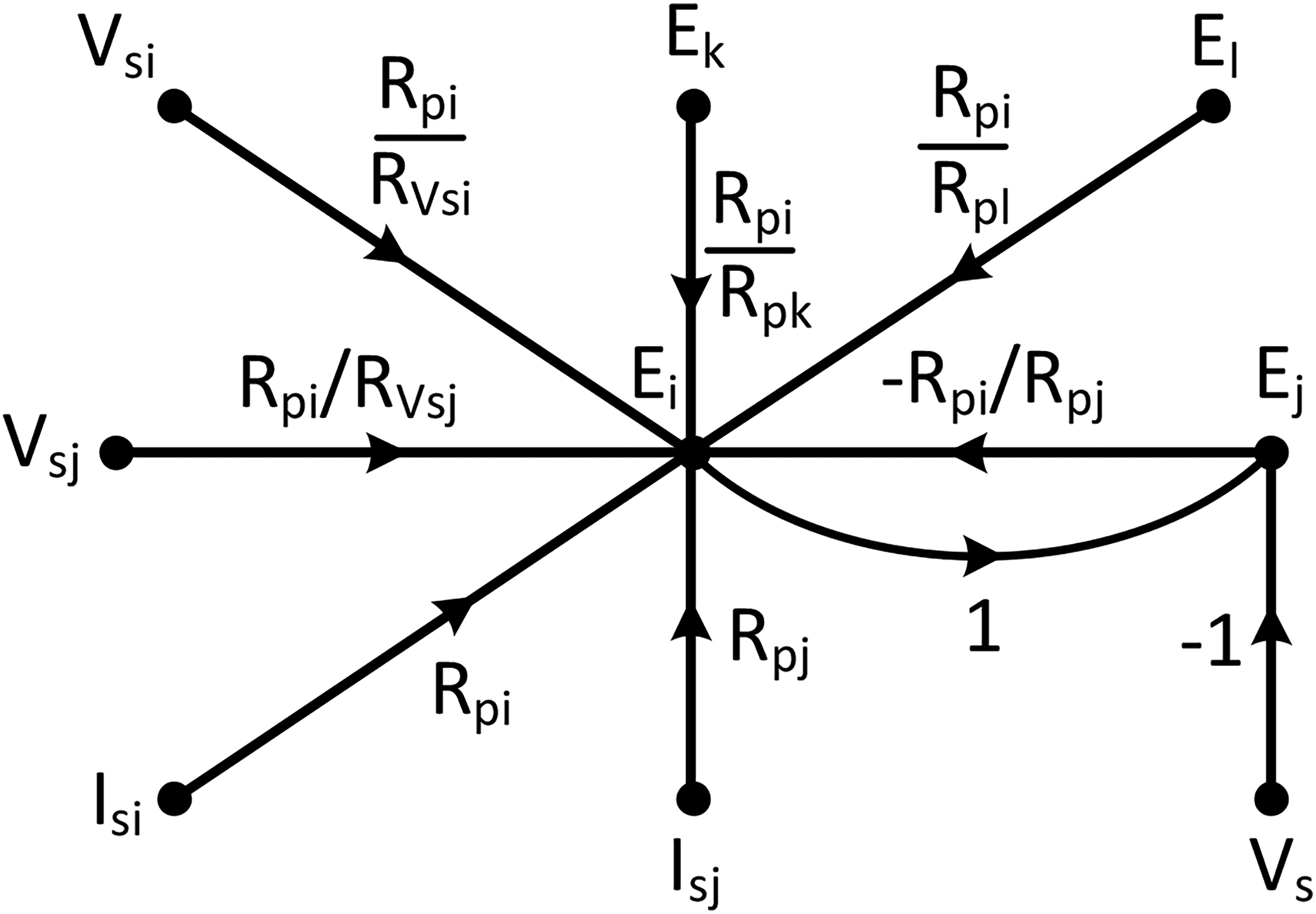
Signal-flow graph of the circuit in Fig. 4.

As a practical example, consider the circuit shown on the left-hand side of Fig. 6. The signal-flow graph can be constructed directly by inspection and is illustrated on the right-hand side of the figure. Node 2 and the current sources contribute gain to node 1. The gain from node 1 to node 2 is unity, while the gain from source V_s to the same node is −1. The equations describing the signal-flow graph are as follows

E_{1} = - \frac{R_{p 1}}{R_{p 2}} E_{2} + R_{p 1} I_{s 1} - R_{p 1} I_{s 2} E_{2} = E_{1} - V_{s}

(26)

where R_p₁ = R₁, R_p₂ = R₂. Solving for the node voltages, we get E₁ = 8.33 V, E₂ = 3.33 V.

Figure 6.

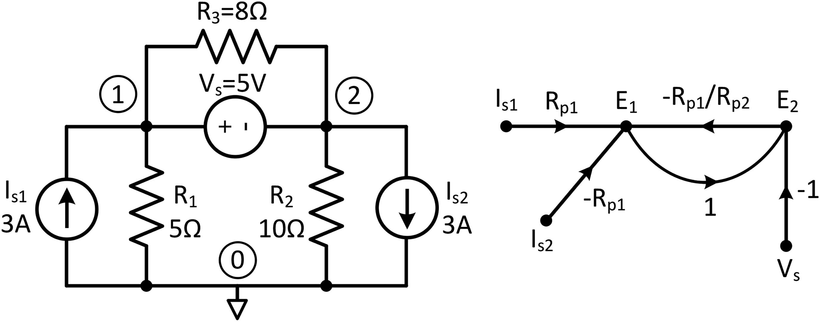
Simple circuit with a floating ideal voltage source.

Calculation of transfer functions with the proposed method

With the node-impedance method, it is relatively easy to calculate transfer functions either in numeric or in symbolic form. As an example, consider the circuit of Fig. 7. The transfer function H(s) = V_o(s)/V_i(s) will be derived following the principles laid out in the previous paragraphs.

Figure 7.

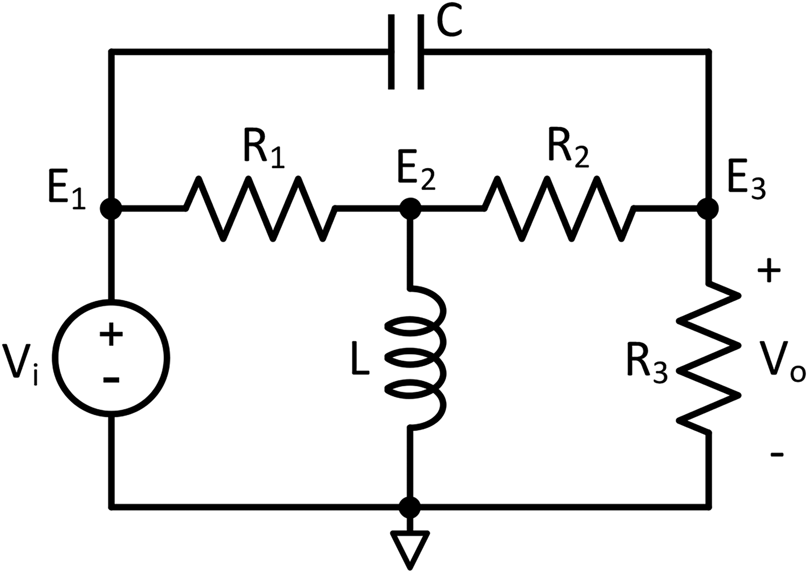
A second order circuit for which the transfer function V_o(s)/V_i(s) is to be determined.

We label the nodes as E₁, E₂, E₃, noting that node E₃ coincides with the output node. The signal-flow graph of the circuit is constructed by inspection, Fig. 8.

Figure 8.

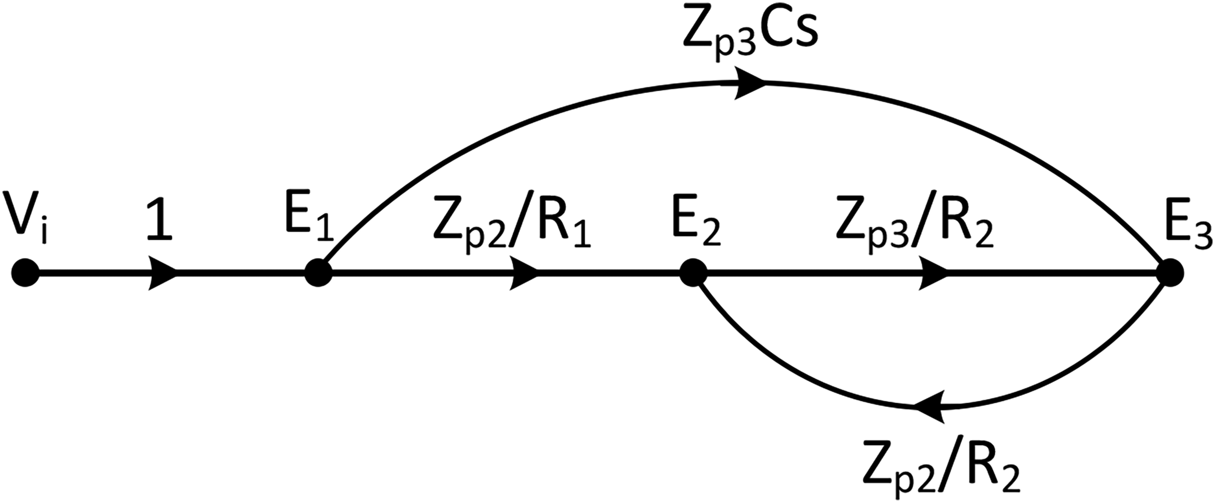
Signal flow graph of the circuit of Fig. 7.

The node impedances are given by the expressions:

Z_{p 1} = R_{1} ‖ \frac{1}{C s} Z_{p 2} = R_{1} ‖ R_{2} ‖ L s Z_{p 3} = R_{2} ‖ R_{3} ‖ \frac{1}{C s}

(27)

Because the signal-flow graph is relatively simple we may use the Mason's algorithm to calculate the gain from V_i to V_o (node 3). There is a single loop L₁ in the graph—from E₂ to E₃ and back to E₂—that is used to form the system determinant Δ as follows:

L_{1} = \frac{Z_{p 2} Z_{p 3}}{R_{2}^{2}} Δ = 1 - L_{1}

(28)

When moving from V_i to E₃ two possible direct paths exist with gains

P_{1} = \frac{Z_{p 2} Z_{p 3}}{R_{1} R_{2}} P_{2} = Z_{p 3} C s

(29)

According to Mason's rule the transfer function is computed as

H (s) = \frac{E_{3} (s)}{V_{i} (s)} = \frac{V_{o} (s)}{V_{i} (s)} = \frac{P_{1} + P_{2}}{Δ}

(30)

By substituting the relative expressions in eqn (30) we get

H (s) = \frac{R_{3} (R_{1} + R_{2}) L C s^{2} + R_{3} (L + R_{1} R_{2} C) s}{R_{3} (R_{1} + R_{2}) L C s^{2} + [(R_{1} + R_{2} + R_{3}) L + R_{1} R_{2} R_{3} C] s + R_{1} (R_{2} + R_{3})}

(31)

Solving circuits with feedback

Circuits that employ feedback, either negative or positive, are more difficult to solve because of the many different signal paths and the return of signals from output to input. Another difficulty arises when we attempt to break the loop; it is a non-trivial task to correctly load the amplifier when the feedback path is opened. By use of the node-impedance method, there is no need to open the loop or assume that the open-loop amplifier and the feedback network are both unilateral. Furthermore, the node-impedance method can solve circuits with multiple feedback loops with no additional effort.

The operational amplifier (op amp) is an electronic device for which the application of feedback is essential for its stable operation. In Fig. 9, two models for the op amp relevant to the application of the node-impedance method are given. The model on the left-hand side is for an op amp with finite voltage gain A, infinite input impedance and zero output impedance. The model on the right-hand side is for an ideal op amp with infinite gain. To ensure that the relation V₊ = V₋ holds a self-loop with gain 1 is added at the output node. The output of an op amp is considered an ideal voltage source; therefore, it accepts no return signals.

Figure 9.

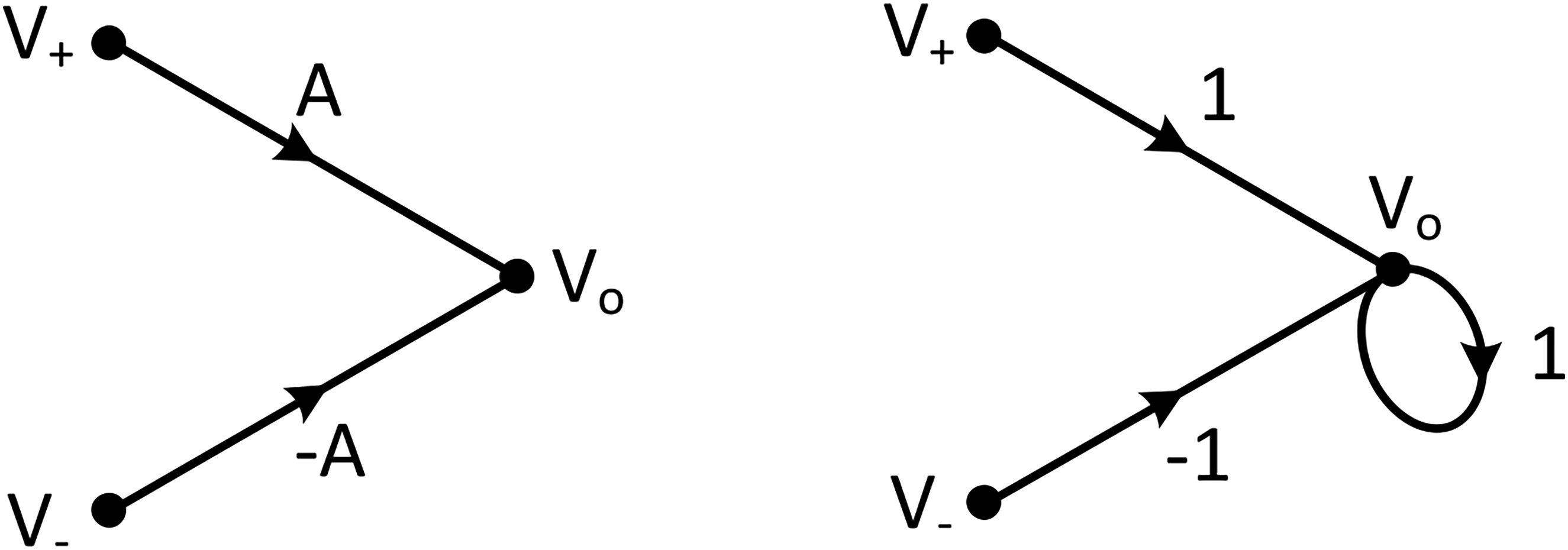
Two possible signal-flow graphs for the operational amplifier. Left: op amp with finite gain A. Right: op amp with infinite gain.

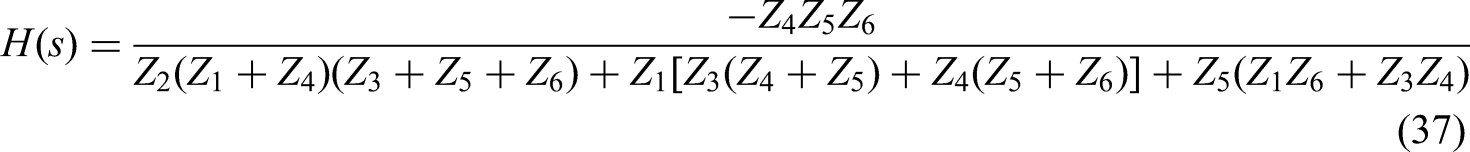
In Fig. 10, a circuit with three feedback loops is depicted where Z₁ – Z₆ are generic impedances. The op-amp is used in its inverting configuration. The aim is to calculate the transfer function H(s) = V_o(s)/V_i(s). The ideal op-amp model with infinite gain of Fig. 9 will be used. The node impedances are given by the expressions:

Z_{p 2} = Z_{1} ‖ Z_{2} ‖ Z_{4} Z_{p 3} = Z_{2} ‖ Z_{3} ‖ Z_{5}

(32)

Z_{p 4} = Z_{3} ‖ Z_{6} Z_{p o} = Z_{4} ‖ Z_{5} ‖ Z_{6}

(33)

where the operator

‖

denotes the parallel combination of the respective impedances.

Figure 10.

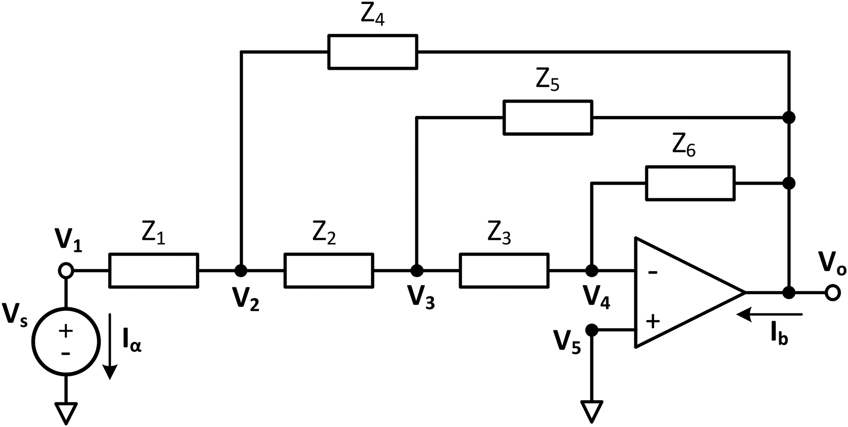
Three feedback loops control the voltage gain of the above circuit. Only the inverting input of the op amp is used, the non-inverting input is connected to ground.

The signal-flow graph is formed by inspection, keeping in mind that the op amp accepts no return signals at its output. We also note that the non-inverting input being grounded contributes no signal to the output and therefore can be omitted.

In Fig. 11 the transmission coefficients are:

a = \frac{Z_{p 1}}{Z_{1}} b = \frac{Z_{p 2}}{Z_{2}} c = \frac{Z_{p 1}}{Z_{2}} d = \frac{Z_{p 3}}{Z_{3}}

(34)

e = \frac{Z_{p 2}}{Z_{3}} f = \frac{Z_{p 2}}{Z_{5}} g = \frac{Z_{p 3}}{Z_{6}} h = \frac{Z_{p 1}}{Z_{4}}

(35)

Figure 11.

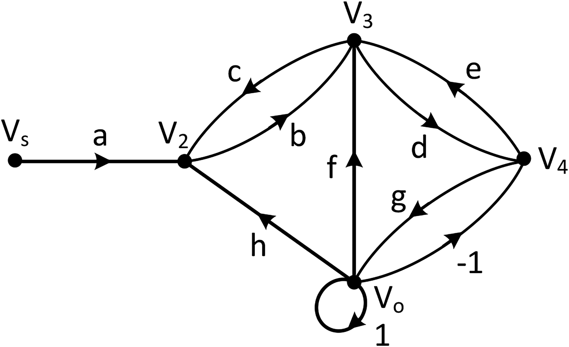
Signal-flow graph for the multiple-loop feedback circuit shown in Fig. 10.

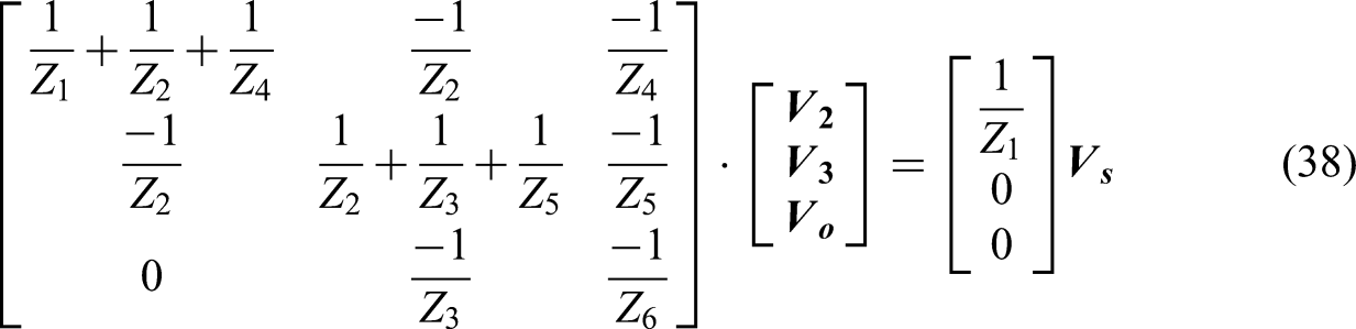
The circuit's equations in matrix form are as follows:

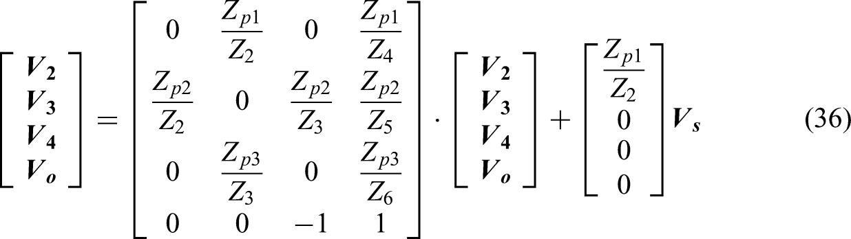
[\begin{matrix} V_{2} \\ V_{3} \\ \begin{matrix} V_{4} \\ V_{o} \end{matrix} \end{matrix}] = [\begin{matrix} 0 & \frac{Z_{p 1}}{Z_{2}} & 0 & \frac{Z_{p 1}}{Z_{4}} \\ \frac{Z_{p 2}}{Z_{2}} & 0 & \frac{Z_{p 2}}{Z_{3}} & \frac{Z_{p 2}}{Z_{5}} \\ 0 & \frac{Z_{p 3}}{Z_{3}} & 0 & \frac{Z_{p 3}}{Z_{6}} \\ 0 & 0 & - 1 & 1 \end{matrix}] \cdot [\begin{matrix} V_{2} \\ V_{3} \\ \begin{matrix} V_{4} \\ V_{o} \end{matrix} \end{matrix}] + [\begin{matrix} \frac{Z_{p 1}}{Z_{2}} \\ 0 \\ \begin{matrix} 0 \\ 0 \end{matrix} \end{matrix}] V_{s}

(36)

Using eqn (11) and solving for V_o(s) we get the desired transfer function.

H (s) = \frac{- Z_{4} Z_{5} Z_{6}}{Z_{2} (Z_{1} + Z_{4}) (Z_{3} + Z_{5} + Z_{6}) + Z_{1} [Z_{3} (Z_{4} + Z_{5}) + Z_{4} (Z_{5} + Z_{6})] + Z_{5} (Z_{1} Z_{6} + Z_{3} Z_{4})}

(37)

At this point, it is instructive to compare the proposed method with the node-voltage method. The node-voltage equations in matrix form are given below

[\begin{matrix} \frac{1}{Z_{1}} + \frac{1}{Z_{2}} + \frac{1}{Z_{4}} & \frac{- 1}{Z_{2}} & \frac{- 1}{Z_{4}} \\ \frac{- 1}{Z_{2}} & \frac{1}{Z_{2}} + \frac{1}{Z_{3}} + \frac{1}{Z_{5}} & \frac{- 1}{Z_{5}} \\ 0 & \frac{- 1}{Z_{3}} & \frac{- 1}{Z_{6}} \end{matrix}] \cdot [\begin{matrix} V_{2} \\ V_{3} \\ V_{o} \end{matrix}] = [\begin{matrix} \frac{1}{Z_{1}} \\ 0 \\ 0 \end{matrix}] V_{s}

(38)

Equations (38) are no more complex than eqns (36); however, they cannot be obtained directly by circuit inspection. Instead, the node equations must first be written out explicitly. Then a simplification can be made by recognizing that, due to the virtual ground, the potential of node 4 is equal to ground. Students inexperienced in circuit analysis tend to make mistakes in this process.

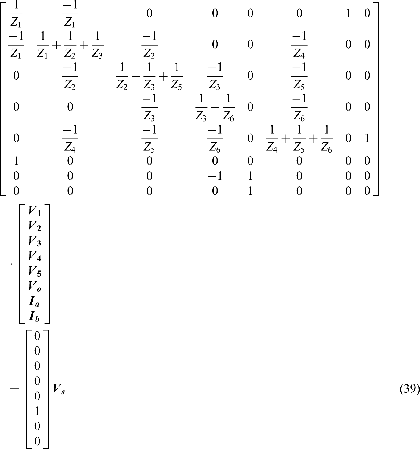
Finally, the MNA equations are given in matrix form (Eqs. 39). In addition to the node voltages, the MNA also uses the current I_α for the ideal voltage source and the current I_b for the output of the op-amp, i.e., a total number of 8 variables. As mentioned earlier, the MNA contains some redundancy. Because each element has its own “stamp” the equations can be written directly. The solution is only possible with the help of a computer.

[\begin{matrix} \frac{1}{Z_{1}} & \frac{- 1}{Z_{1}} & 0 & 0 & 0 & 0 & 1 & 0 \\ \frac{- 1}{Z_{1}} & \frac{1}{Z_{1}} + \frac{1}{Z_{2}} + \frac{1}{Z_{3}} & \frac{- 1}{Z_{2}} & 0 & 0 & \frac{- 1}{Z_{4}} & 0 & 0 \\ 0 & \frac{- 1}{Z_{2}} & \frac{1}{Z_{2}} + \frac{1}{Z_{3}} + \frac{1}{Z_{5}} & \frac{- 1}{Z_{3}} & 0 & \frac{- 1}{Z_{5}} & 0 & 0 \\ 0 & 0 & \frac{- 1}{Z_{3}} & \frac{1}{Z_{3}} + \frac{1}{Z_{6}} & 0 & \frac{- 1}{Z_{6}} & 0 & 0 \\ 0 & \frac{- 1}{Z_{4}} & \frac{- 1}{Z_{5}} & \frac{- 1}{Z_{6}} & 0 & \frac{1}{Z_{4}} + \frac{1}{Z_{5}} + \frac{1}{Z_{6}} & 0 & 1 \\ 1 & 0 & 0 & 0 & 0 & 0 & 0 & 0 \\ 0 & 0 & 0 & - 1 & 1 & 0 & 0 & 0 \\ 0 & 0 & 0 & 0 & 1 & 0 & 0 & 0 \end{matrix}] \cdot [\begin{matrix} V_{1} \\ V_{2} \\ V_{3} \\ V_{4} \\ V_{5} \\ V_{o} \\ I_{a} \\ I_{b} \end{matrix}] = [\begin{matrix} 0 \\ 0 \\ 0 \\ 0 \\ 0 \\ 1 \\ 0 \\ 0 \end{matrix}] V_{s}

(39)

Conclusion and future work

The node-impedance method has been proposed as an alternative to traditional methods of circuit analysis. It is capable of solving a wide range of problems with no additional steps and minimal complication. The transfer gains between nodes, automatically generated by this method, facilitate the construction of the signal-flow graph. Applications include solving all types of circuits in DC, AC or the s domain, the calculation of transfer functions and solving circuits with feedback.

The method has been used in class for the last 5 years with positive results. Students familiarize themselves quickly with the particularities of the method and are able to write down the equations of complicated circuits.

The method's ability to solve circuits with more than one feedback loops has been demonstrated; however, more work is under way in this direction to compute the return ratio, the loop gain and other metrics specific to circuits using feedback. In addition, more work needs to be done to handle circuits containing mutual inductances and ideal transformers.

Footnotes

Acknowledgements

The author gratefully acknowledges the anonymous reviewers whose precise and constructive comments significantly improved the final version of the paper.

ORCID iD

Spyros Loutridis

Funding

The author received no financial support for the research, authorship, and/or publication of this article.

Declaration of conflicting interests

The author declared no potential conflicts of interest with respect to the research, authorship, and/or publication of this article.

References

Ruehli

Brennan

. The modified nodal approach to network analysis. IEEE Trans. Circuits Syst 1975; 22: 505–509.

Shannon

. The theory and design of linear differential equation machines. Report, Fire Control of the US National Defense Research Committee: Report no 411, Section D-2 January 1942.

Mason

. Feedback theory - some properties of signal flow graphs. Proceedings of the IRE 1953; 41: 1144–1156.

Coates

. Flow-Graph solutions of linear algebraic equations. IRE Trans. on Circuit Theory 1959; 6: 170–187.

Choma

. Signal flow analysis of feedback networks. IEEE Trans. on Circuits and Systems 1990; 37: 455–363.

Grimbleby

. Symbolic analysis of circuits containing active elements. Electronic Letters 1981; 17: 754–756.

Leach

. On the application of Thevenin and Norton equivalent circuits and signal flow graphs to the small-signal analysis of active circuits. IEEE Trans. on Circuits and Systems 1996; 43: 885–893.

Jung

Song

Cressler

. Systematic Methodology for Applying Mason’s Signal Flow Graph to Analysis of Feedback Circuits. In: 2014 IEEE International Symposium on Circuits and Systems (ISCAS 2014), Melbourne, Australia, 01-05 June 2014, pp.2421–2424. IEEE.

Kelly

. Electronic circuit analysis and design by driving-point impedance techniques. IEEE Trans. on Education 1970; 13: 154–167.

10.

Asamoah

. Analysis and design of analogue electronic circuits using DPI methods – part 1. Int. J. Electr. Eng. Educ 1991; 28: 174–182.

11.

Ochoa

. Loop Gain in Feedback Circuits: A Unified Theory Using Driving Point Impedance. In: 2013 IEEE 56th International Midwest Symposium on Circuits and Systems (MWSCAS), Columbus, OH, USA, August 4-7, 2013, pp.612–615. IEEE.

12.

Schmid

. Circuit Transposition Using Signal-Flow Graphs. In: 2002 IEEE International Symposium on Circuits and Systems. Proceedings (Cat. No.02CH37353). Phoenix-Scottsdale, 26-29 May 2002, paper no. 0-7803-7448-7/02.

13.

Biolek

Biolková

. Flow Graphs Suitable for Teaching Circuit Analysis. In: AEE’ 05: Proceedings of the 4th WSEAS International Conference on Applications of Electrical Engineering, March 13-15, 2005, pp.33–35. WSEAS.