Comparison between experimental and theoretical results using Cuntze’s “failure mode concept” model for composites under triaxial loadings—Part B of the second world-wide failure exercise

Abstract

This paper represents a comparison between the predictions of Cuntze’s Failure Theory, referred to as ‘failure mode concept model, and experimental results provided in Part B of the second World-Wide Failure Exercise. The results covered 12 test cases, involving an isotropic matrix material, 7 UD laminas and 4 multi-directional laminates subjected to 3D states of stress. The UD lamina data, needed for the validation of the failure mode concept-based UD strength conditions, were broadly applicable, whereas the laminate data could only partly serve for model verification because some test cases show some discrepancies. Also, there was a lack of test data in some of the test cases and it is concluded that there is a need to obtain more representative test data. Nevertheless, a good mapping could be achieved by the applied strength conditions dedicated to the specific test case.

Keywords

UD-lamina failure conditions tri-axial stressing hydrostatic compression multi-directional laminates non-linear behaviour

Introduction

Proving the capability of the tri-axial failure mode concept (FMC) theory requires realistic, well-evaluated and well-understood experimental data. In an attempt to achieve that, the author has made a contribution to Part A of the second World-Wide Failure Exercise (WWFE-II), Part A, with the aim of assessing the capability of the FMC model for predicting failure in composite laminates under tri-axial stresses, see Reference [3]. In the present paper, and as a contribution to Part B of the WWFE-II, the author and originator of the FMC makes a comparison between the theoretical predictions for 12 different test cases (TC) and experimental results provided by the organisers of the WWFE-II.^4,5

The paper starts with providing a description of the experimental data provided and their origin. Comments are then made about the usefulness of the data and the testing techniques used to generate the experiments. The correlation between the theory and the experiments is then described.

It was found that it was necessary to modify the Mohr-Coulomb required material friction parameter (not provided, had to be estimated in Part A) in order to capture trends exhibited by the experimental results. Also, the matrix model was improved despite the fact that the matrix data seems not to exhibit a 2ndTg-effect. Finally, first with the delivery of the Part B test data, an average stress–strain curve could be determined, which is required to accurately perform the TC2, TC3 and TC4 analyses.

Cuntze’s failure mode concept-based failure theory

General

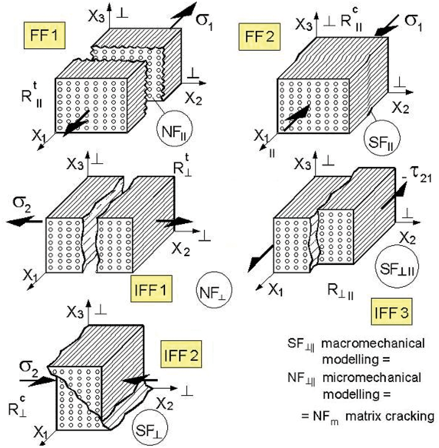
The model (see References [3,6]) involves the following: (a) proposing appropriate non-linear stress–strain curves for the UD lamina before and after occurrence of initial failure (interfibre-failure [IFF]), (b) taking into account the effect of pressure on mechanical properties and (c) incorporating five failure distinct modes (two fibre-failure (FF) and three IFF, see Figures 1 and 2), into a single equation.

Figure 1.

Tri-axial state of stress, acting at a matrix material and a UD material cube. For lamina coordinate and fibre orientation angle, see second World-Wide Failure Exercise (WWFE-II) Part A.³

Figure 2.

Failure mode concept (FMC) view of the fracture types of brittle transversely isotropic UD material.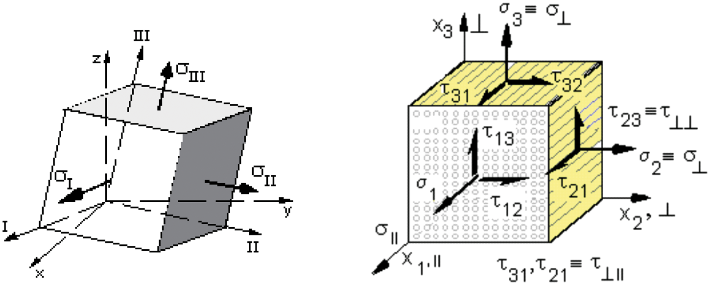

For the UD material element, Figure 1 depicts the 3D state of stress ${σ} = (σ_{1}, σ_{2}, σ_{3}, τ_{23}, τ_{31}, τ_{21})^{T}$ . Because of the symmetries of the transversely-isotropic UD material, only five basic strengths and five elasticity properties are needed. Therefore, the characterisation of strength requires the measurement of five independent basic lamina strengths (in brackets the US denotation):

– $R_{| |}^{t}$ (= $X^{t}$ ) and $R_{| |}^{c}$ (= $X^{c}$ ) as tensile and compressive strength parallel to the fibres;

– $R_{⊥}^{t}$ (= $Y^{t}$ ) and $R_{⊥}^{c}$ (= $Y^{c}$ ) as tensile strength and compressive strength transversal to the fibre direction); and

– $R_{⊥ | |}$ (=S) as in-plane shear strength.

Fibre orientation is defined as positive when the angle is measured from the x direction to fibre direction (x₁).

Hence, a full non-linear failure analysis of 3D states of stress is understood here to involve four distinct parts:

Failure conditions to assess multi-axial states of stress (see Figure 1),

Non-linear stress–strain curves of the UD lamina material as input (see Part A),

Non-linear coding for obtaining a realistic response of the laminate and

Incorporation of the effects of the ‘hydrostatic pressure’.

Assumptions for modelling in the WWFE-II

Key features of the FMC, published in WWFE-II, Part A, are listed in Table 1. In order to be able to apply these features to solve problems involving triaxial loadings, the following assumptions have been considered:

– Pore-free material, specimen surfaces polished and well sealed

– Fibre volume content is constant ( $V_{f} = 60$ %)

– Perfect bonding between adjacent layers is assumed here, neglecting layer waviness and edge effects

– The incorporation of the effects of the 2ndTg shift on the behaviour of a lamina has been carried out through the use of suitable micro-mechanical equations.

– A linear relationship is used to describe the softening (decrease of the slope) of the modulus and the shear strength of the matrix as a function of pressure.

– The UD lamina is assumed to be transversely isotropic and behaves in a brittle manner. This matches with Part A and the provided UD test data

– The fracture type, referred to as normal fracture (NF) or shear fracture (SF) in Figure 2, depends on the model level: For IFF3, the fracture type may be an NF (constituent micro-level) or a SF (lamina macro-level).

Table 1.

Main features of the failure mode concept (FMC) and associated non-linear analysis

• Each mode represents one theoretically independent failure mechanism and one piece of the complete failure surface (surface of the failure body or so-called limit surface)

• Each failure mechanism is represented by one failure condition. One failure mechanism is governed by one basic strength and therefore has a clearly defined equivalent stress σ_eq and a material stressing effort Eff to be used at least in the (non-linear) progressive damage analysis

• An invariant formulation of a failure condition – in order to achieve a beneficial scalar formulation considering the material's symmetries – is possible

• For each mode one material stressing effort can be determined, displaying, where the design key has to be turned and linking highest material stressing effort to highest risk

• The invariant term in the failure condition can be related to a physical mechanism observed, when it causes a volume change or a shape change of the solid material element or ‘internal friction’

• Curve-fitting of the course of test data is only permitted in each pure regime of a failure condition

• Rounding-off in mode interaction zones is performed by a spring model. This means a rounding-off of adjacent mode failure curves (partial surfaces) in their interaction zone which is leading again to a global failure curve (surface), or in other words, to a ‘single surface failure description‘, such as with Tsai/Wu, however, without its well-known shortcoming

• Failure mode identification is mandatory for a progressive failure analysis in order to know how the lamina has failed. This makes a clear degradation of the elastic moduli possible.

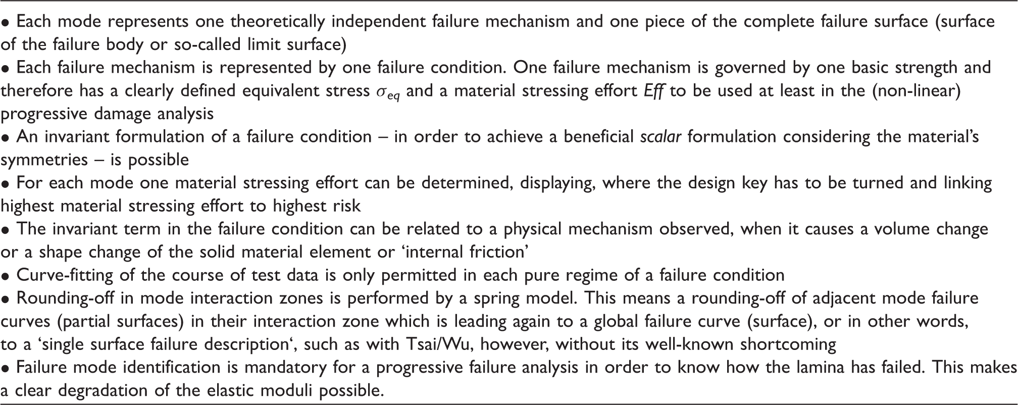
Details of possible refinements of the analysis and changes in modelling

FMC-based failure conditions and non-linear analysis

Due to a change in the given matrix behaviour (Part A: information yielding; B: information fracture), matrix modelling was changed from ductile to semi-brittle behaviour.

The non-linear analysis used here is the same as in Part A, where a secant-modulus procedure was adopted. A simple MathCad 13 code was used.

Re-work of the matrix model in ultra-high compression domain

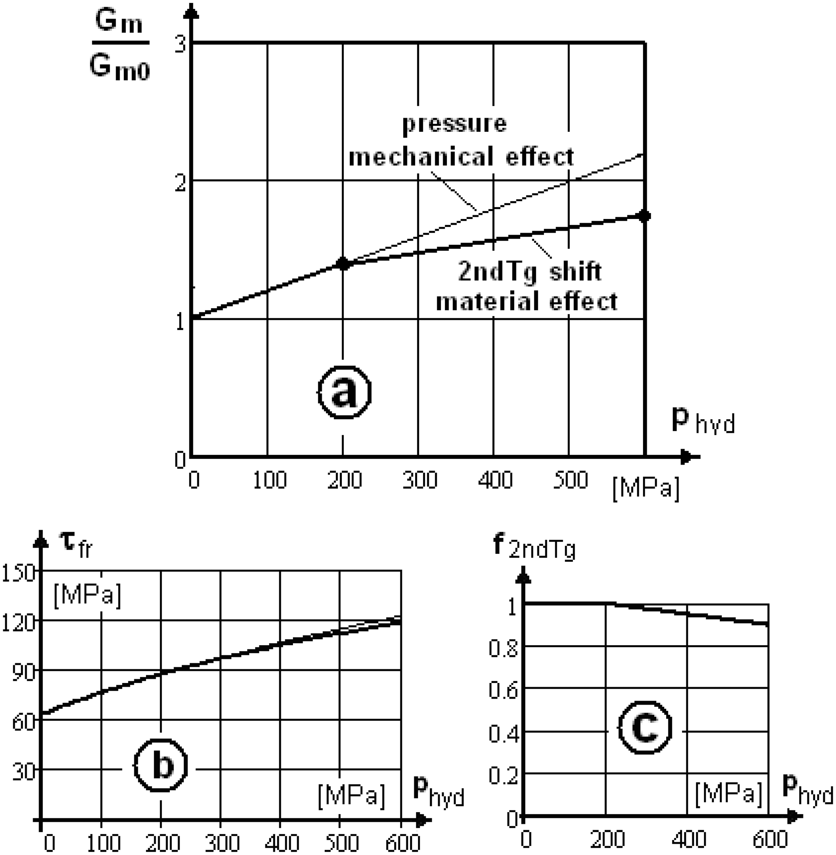
Considering elastic stiffness, from the various cited references a semi-empirical approach can be constructed on basis of previously published test results for the shear modulus, References [7, Figure 5; 8]. The kinked curve in Figure 3 can be fitted with a bi-linear manner function (series spring model) as follows:

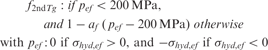
\begin{matrix} f_{2 nd Tg} : if p_{ef} < 200 MPa, \\ and 1 - a_{f} (p_{ef} - 200 MPa) otherwise \end{matrix}

(1)

with $p_{ef}$ : 0 if $σ_{hyd, ef} > 0$ , and $- σ_{hyd, ef}$ if $σ_{hyd, ef} < 0$

with $a_{f}$ as fitting parameter, representing the decay of the slope in Figure 3, and the reduction factor $f_{2 nd Tg}$ . The effect on the moduli at room conditions can be tackled by

G_{m} = G_{m 0} \cdot f_{2 nd Tg} with G_{m 0} = E_{m 0} / (2 + 2 \cdot ν_{m 0}) .

(2)

Figure 3.

(a) 2ndTg shift effect: Dependence of the matrix shear modulus on p _hyd . Assumption for PR319: knee point 200 MPa at ratio 1.4; final point 600 MPa at ratio 1.75, see Reference [15]). (b) Distribution of fracture stress. (c) Decay function $f_{2 nd Tg}$ due to 2ndTg shift.

Figure 5.

TC1: Tri-axial compressive failure stress curve $σ_{x, fr} (σ_{y} = σ_{z})$ of the MY750 epoxy resin matrix. ${\bar{R}} = ({\bar{R}}_{t}, {\bar{R}}_{c})^{T} = (80, 120)^{T} MPa, R_{τ} = 54 MPa, b_{τ}^{c} = 0.18 .$ R_tt, (R_ttt) = bi-axial (tri-axial) tensile strength. Open failure surface.

To be inserted into this equation is the effective hydrostatic stress $σ_{hyd, ef}$ in the constrained matrix material point at the envisaged critical location within the embedded constrained lamina. The decay of the slope of stiffness and ‘strength’ in the ultra-high hydrostatic domain was tackled in Part A by a blind preliminary approach which used the mean stress in the matrix material as effective hydrostatic stress $σ_{hyd, ef} = I_{1} / 3 = - p_{hyd, ef}$ . This had to be refined in order to tackle the usually different normal stresses. Hence, the approach was changed in Part B to the equations (3) as improved engineering approach to capture the 2ndTg-effect

σ_{ef, m} = max (σ_{1, m}, σ_{2}, σ_{3}) .

(3a)

In the case of tri-axial and lateral bi-axial compression ( $σ_{2}, σ_{3}$ ) of a lamina, the state of stress $σ_{1, m}$ in the fibre-constrained matrix has to be used. It is generated because the stiff fibres prevent a free matrix elongation and build up an effective hydrostatic compression stress in the matrix. Micro-mechanical equilibrium leads to the relationship

σ_{1, m} = - σ_{f} \cdot V_{f} / (1 - V_{f}) = - ɛ_{1} \cdot E_{| |} \cdot V_{f}^{2} / (1 - V_{f})

(3b)

employing

σ_{f} = ɛ_{1} \cdot E_{| |} \cdot V_{f}

. The mathematically highest stress is effective. Both quantities,

σ_{ef, m}

and

σ_{1, m}

, are sign-dependent. This means, pressure is inserted as a negative value and a hydrostatic tensile stress as a positive value. Unfortunately, the author could not validate the equations (3) by the provided test information.

Transfer to UD stiffnesses and UD strengths

For the UD material, the 2ndTg-effect will differ from that which is obtained for the pure matrix, the effect is usually minor. However in the TC, lacking of knowledge for the UD materials, the strength reduction factor $f_{2 nd Tg}$ might be simply transferred from the matrix to the multi-axial UD fracture stresses.

‘Strength’ decrease and ‘healing’

According to the usual failure condition $σ_{eq} ({σ}) / \bar{R} = 1$ , the load-carrying capacity can formally increase with a ‘lower’ $σ_{eq}$ -value and with a higher strength $\bar{R}$ . Therefore, the beneficial multi-axial pressure-based lowering of the equivalent stress $σ_{eq}$ should be not mixed up with an increase of a measured material property $\bar{R}$ .

With respect to a ‘healing’ of the ‘diffuse’ micro-cracking situation, the effect of pressure is inherent in the lamina and the laminate high pressure test data (e.g. TC 2). It needs to be separately modelled, whenever applicable.

Consideration of in-situ effect of the embedded lamina

Properties used as input (see e.g. Reference [9]) for the analysis are test results from isolated UD lamina specimens such as a tensile coupon. They are load-controlled derived and results of weakest link type, whereas the in-situ behaviour of an embedded UD lamina is deformation-controlled and therefore of redundant type. This fact shows up that a good mapping of the course of ‘isolated UD test data’ does not involve the full information necessary for a qualified post-IFF analysis of laminates, which consist of a stack of embedded laminas.

Brief descriptions of test cases and comments on Part B test data provided

Description of test specimens

In this paper, an attempt is made to validate a theoretical model of the reality by some experimental realisations of the reality. To accomplish this, 12 challenging TC are provided by the WWFE-II organisers⁵ involving (see Table 4 in Part A):

Epoxy material under a tri-axial state of stress

0° unidirectional lamina under various tri-axial states of stress

[0/90]_s, [±45/90/0]_s, [±35]_s multi-directional laminates under various tri-axial states of stress and through-thickness loadings and

three stress–strain curves for

– 0° unidirectional laminas under various tri-axial states of stress

– [±35]_s laminates under a tri-axial state of stress and

– [0/90]_s laminates under through-thickness compression.

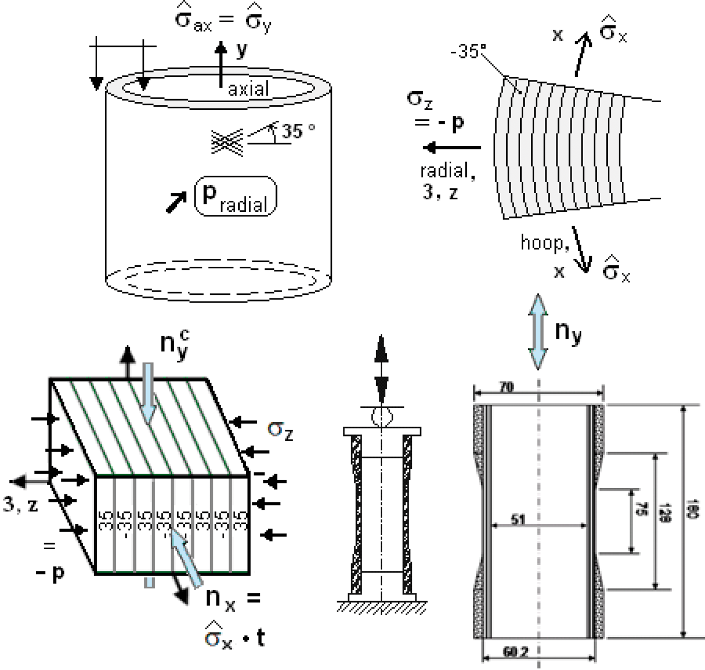
Different shapes of the test specimens were used in the experiments. These are as follows:

For TC1, a solid cylinder specimen

For TC 2,3,4,8,9: thick-walled tubes,

For TC5: a rectangular block,

For TC6,7: dog-bone-shaped machined specimens from pultruded rods,

For TC10,11 waisted (dog-bone shaped) tubes milled from a laminate block and

For C12: waisted solid laminate specimen.

Test results for TC2 and TC3, obtained from 0° pin-wound tubes, were also provided by the organisers. However, these results cannot be used (see Annex 5) for the validation of the UD strength conditions, just the data from the hoop-wound tubes are applicable.

Above variations in test specimens (manufacture etc.) have different effects on the quality of the validation. In total, nine different tri-axial failure domain envelopes and three stress–strain curves have to be correlated.

Comments on experimental input

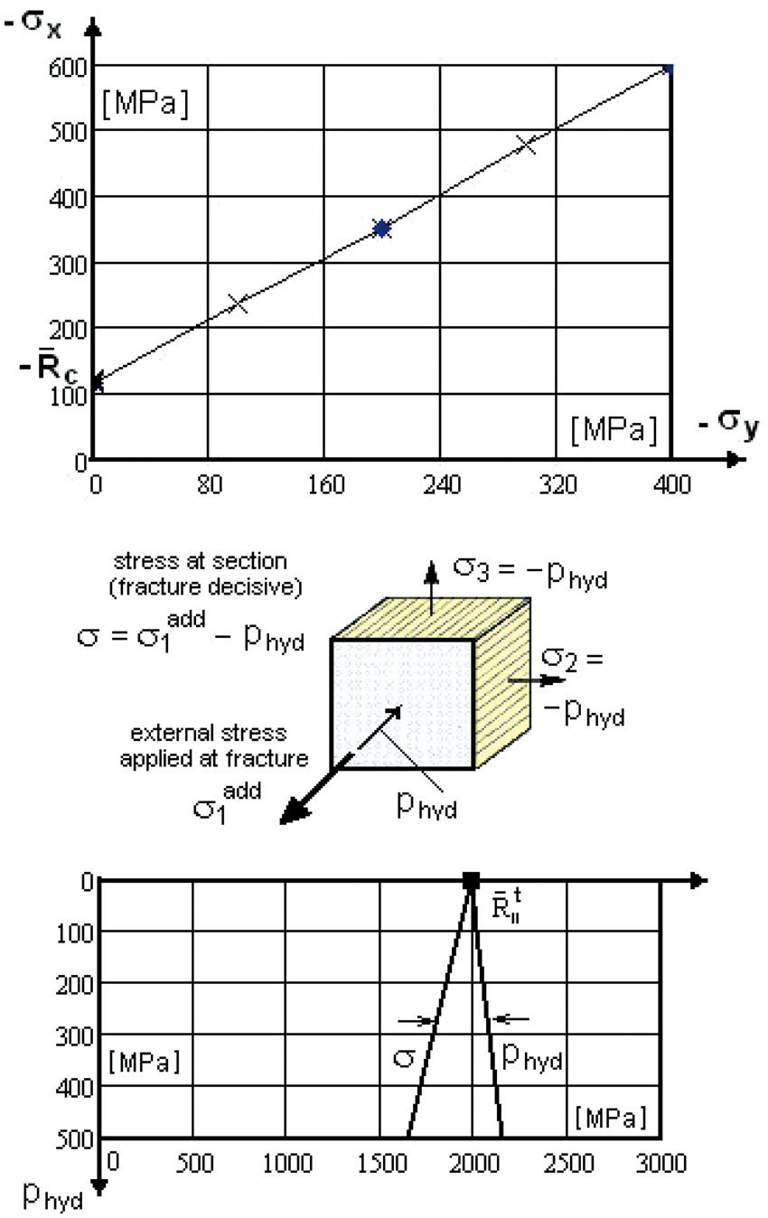
Making an attempt to understand the provided experimental results one has to distinguish whether the test results are fracture values in total stresses or hydrostatic pressure superposed fracture stresses. This difference is not always clearly expressed in the given test information. From comparing data of various sources one can only sort out What might be meant? Due to Figure 4, for the example UD lamina, tri-axial failure information can be provided in several ways ( $σ_{hyd} = - p_{hyd}$ ) of the state of stress:

\begin{matrix} {σ} = (σ_{1}, σ_{2}, σ_{3}, τ_{23}, τ_{31}, τ_{21})^{T} or \\ {σ} = (σ_{1}^{add} - p_{1}, σ_{2}^{add} - p_{2}, σ_{3}^{add} - p_{3}, τ_{23}, τ_{31}, τ_{21})^{T} or \\ {σ} = (σ_{1}^{add} - p_{hyd}, σ_{2}^{add} - p_{hyd}, σ_{3}^{add} - p_{hyd}, τ_{23}, τ_{31}, τ_{21})^{T} \end{matrix}

(4 a,b,c)

with the pressures

p_{i}

as absolute pressure values, acting at a cross-section surface. The stresses

σ^{add}

are the additional stresses which may be increased up to

σ_{fr}^{add}

. This is the resistance value that marks the pressure-dependent multi-axial fracture state of stress.

Figure 4.

Transfer of experimental data in compressive and tensile domains. x = provided data, parallelogram = transformed data.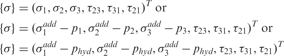

In order to correctly interpret the diagrams in the associated literature, one has to carefully check whether the diagram is of the type $σ_{x, fr} (σ_{y} = σ_{z}, \bar{R})$ or of $σ_{x, fr} (p_{hyd}, \bar{R})$ . Figure 4 proves that the data are identical.

In order to interpret and use the test data (not all are clear) correctly, it is of basic interest to understand what is behind, what are the test specimens and the test rig (examples TC 10, 11). In this context, TC tests, test specimens and test data are commented in detail in the next chapters beginning with some “linformation phrases” typical for the TC.

Discussion of test data and associated information provided for Part B

Basic material properties are provided in Annex 3 TC1: $σ_{x, fr} (σ_{y} = σ_{z})$ , matrix MY750epoxy (Figure 5)

“Test data from a sealed cylindrical bar epoxy specimen in a container filled with a highly pressurized fluid. ¹⁰ The axial loading is carried out by a pull rod. The necessary two seals cause friction which is considered in the provided fracture stress data. The axial fracture stress is computed from the measured load divided by the original cross-section”.

Barrelling was not monitored! Not all physically needed properties, such as the (low) material friction of this semi-brittle matrix material, could be provided by the organisers.

– The course of the provided test data does not exhibit the 2ndTg-effect demonstrated by a slope beyond the epoxide-typical −200 MPa (hydrostatic pressure, equal compressive stresses) kinking point, Figure 5a. This of course also meets the 2ndTg-matrix modelling under a general 3D compression loading with different stresses in the three coordinate directions. Information for modelling the change of stiffness and ‘strength’ is not directly given, and in literature the data vary. Therefore, a correction factor $f_{2 nd Tg}$ has to be assumed for stiffness and for ‘strength’ as well. If applicable for a distinct TC, both, for stiffness and ‘strength’ the same value is taken, namely an assumed 10% decay of the slope between −200 MPa and (pretty arbitrarily) −600 MPa.

Unfortunately, literature could not fill the lack of information. Instead, a discrepancy was found: Beyond the kinking point, Young’s modulus E still increases in Reference [10] with a distinct (lower) slope, whereas in References [7,8,11,12], the related shear modulus $G_{m}$ is decreasing. Of course, there is no strong relationship between E and G anymore ( $E \neq G \cdot (2 + 2 \cdot ν)$ ), but, also Birch’s formulas (Part A) do not confirm such a different behaviour.

– In Reference [10], it is reported: All test specimens under compression failed by yielding (for Part B the failure type yielding was corrected by the reviewer into fracture which is essential). This holds from atmospheric pressure up to $p_{hyd} = 400 MPa$ . The failure description in the compression domain will be modelled by a low b friction parameter value of $b_{τ}^{c} = 0.18$ . Note that $b_{τ}^{c} (μ = 0) = 0$ means ‘Mises yield cylinder’ and full yielding.

– The provided dataset forms a straight line and thereby does not show any 2ndTg-effect, Figure 5(a). On the contrary, beyond the indicated kink level (at about −200 MPa) the Figure 5(c) shows a widening of the failure surface instead of a shrinking. It looks as if the effect needs not to be addressed for this matrix material. Nevertheless, for a visualisation of the tendency of the 2ndTg shift effect a 10% slope decay is assumed and displayed in the Figures 5a and 5c.

Note: In Figure 5(c), so-called Lode coordinates $I_{1} / (\sqrt{3} \cdot {\bar{R}}_{c})$ and $\sqrt{2 \cdot J_{2}} / {\bar{R}}_{c}$ are applied. They have the advantage to possess the same scale in the full stress space.

Modifications from Part A to Part B: As the providers have changed the information on the matrix behaviour from yielding to fracture the friction model parameter $b (μ)$ had to be increased for Part B. No change of the FMC model itself must be made.

TC2: $τ_{21}^{fr} (σ_{2} = - p_{hyd})$ , UD T300-PR319epoxy (as for TC3, TC4) (Figures 6 and 7)

Figure 6.

TC2: Fracture stress $τ_{21, fr}$ vs stress $σ_{2} (= σ_{1} = σ_{3} = - p_{hyd})$ for a UD T300 carbon/PR319 epoxy hoop wound tube, $σ_{hoop} \equiv σ_{1}$ , $σ_{3} \equiv σ_{radial}$ . ${\bar{R}} = (1378,_{} 950,_{} 40,_{} 125,_{} 97)^{T}$ MPa. ${E} = (129000,_{} 129000,_{} 5600,_{} 5600,_{} 1330)^{T}$ MPa. $ν_{⊥ | |} = 0.32$ , m = 2.8, $b_{⊥ | |} = 0.12$ . $ν_{23} = 0.48$ , $G_{23} = 1860 MPa$ ); Check point: $γ_{21} = 0.142,^{} τ_{21} = 140 MPa,^{} p_{hyd} = 600 MPa$ .

Figure 7.

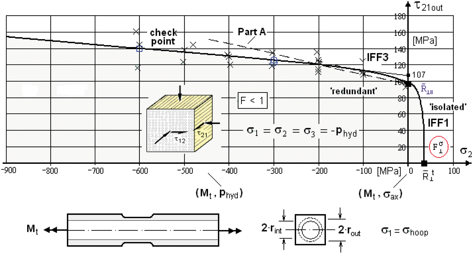
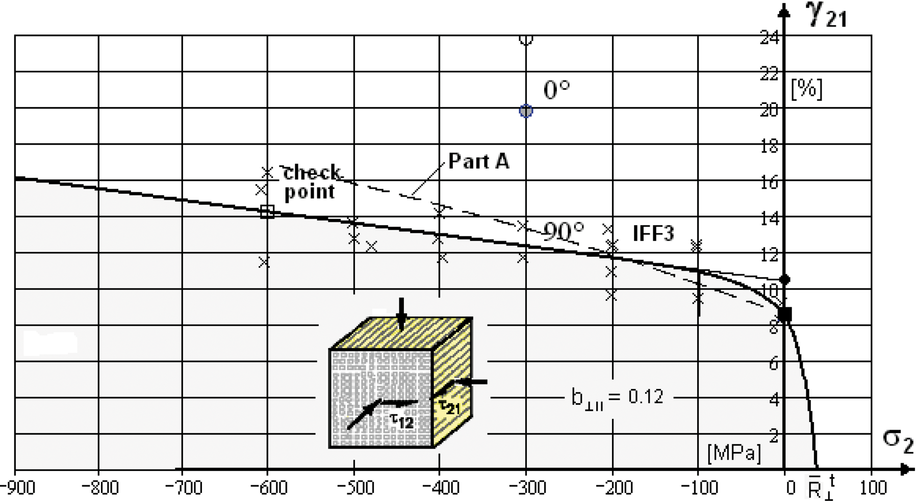
TC3: Failure shear strain $γ_{21} (σ_{2} = - p_{hyd})$ in dependence of an increasing p_hyd. UD T300 carbon/PR319 epoxy hoop wound tube. Properties, see TC2. Two 0° test data (circles) are shown for information and Annex 5 calculation. Part A curve: $b_{⊥ | |} = 0.3$ (dashed).

The test results obtained from the two test specimen types show wide scatter and jumping. Test data does not show a 2ndTg-effect. Investigated are only the 90° tubes. An investigation, why the data set of the twisting 0° tube is not used (see Figure 8), is performed in Annex 5.

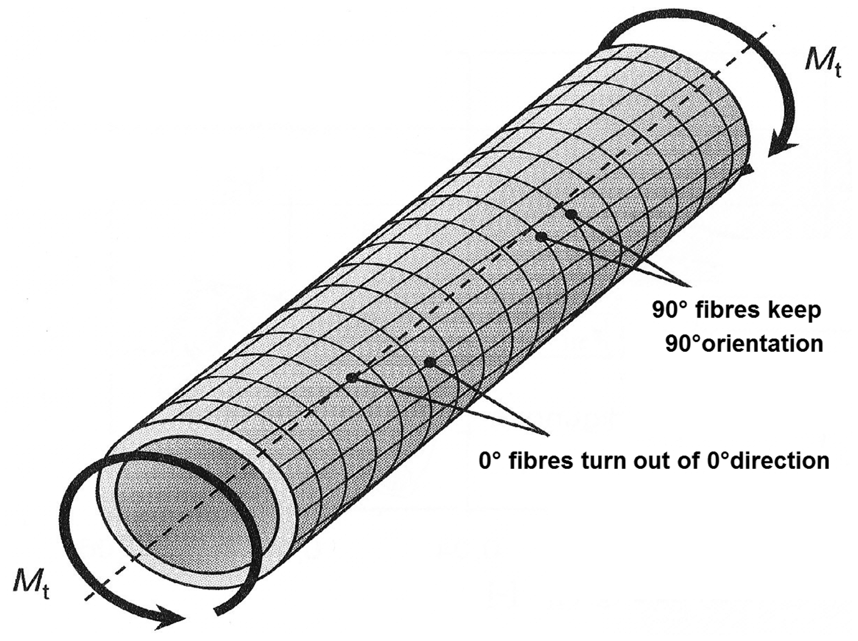
– The tubes are relatively thick-walled. This means for torsion that the shear stress grows from inner to outer radius. Therefore, $τ_{out}$ is failure-responsible. The shear strength increases from the inner to the outer radius according to the following formula (see Reference [13]) $τ = 2 \cdot M_{T} \cdot r / [π \cdot r_{out}^{4} \cdot (1 - r_{inn}^{4} / r_{out}^{4})]$ , and $τ_{out} ≅ 1.4 \cdot τ_{inn}$ . It is assumed that $τ_{out}$ is the provided shear stress. For information, the application of the shear stress formula for the thin-walled tube delivers a $τ_{thin} = 0.88 \cdot τ_{out}$ , which is a smeared value. So, the outer wall surface is the critical location.

Figure 8.

Change of the fibre orientation under torsion in TC2, TC3 (courtesy IKV Aachen²⁶).

For the other critical stress, the filament hoop stress and its strain $ɛ_{f} \equiv ɛ_{| |}$ , the critical radial location has to be sorted out, whether it lies at the inner radius or at the outer radius. Due to the elastic behaviour in radial direction, the hoop stress $σ_{1}$ changes from a positive value at the inner radius to an outside negative compressive value. However, not $σ_{1}$ is responsible for fracture but $σ_{1 f}$ . This means, $σ_{1}$ has to be replaced by ${\overset{⌣}{σ}}_{1} ≅ ɛ_{| |} \cdot E_{| |}$ to simply achieve that.

– A Finite Element Analysis check delivered a filament hoop strain at about $ɛ_{fr}^{| | t} = - 0.74 %$ and an extreme stress gradient. This means that shear fracture IFF3 may be overtaken at the $p_{hyd} = 600 MPa$ level (the large scatter backs this up) by a relative sudden occurring FF2. Also, structural collapse may occur. Closing of the failure surface will be the result of the common actions of material failure FF2 and structural failure of the tube.

Theoretically from simple elastomechanics, the hydrostatically loaded tube will break at

p_{hyd} = R_{| |}^{c} / (1 - 2 \cdot ν_{⊥ | |}) = 950 / (1 - 2 \cdot 0.32) = 2600 MPa .

This is a guess if the tube remains structurally stable and if the Poisson’s effect causing

ν_{⊥ | |}

remains constant. A consideration of the unknown 2ndTg effect will terminate the curve earlier.

– Novel idea: (1) At a first look, the jump in data size at $σ_{2} = 0$ or at shear strength $R_{⊥ | |}$ is not clear because it is the same shear failure mode IFF3. An explanation for the jump is the ‘healing’ or the redundantly acting hydrostatic pressure effect. In order to fit the course of data on an average the shear strength is increased up to a model value of $107 MPa$ regarding redundancy. (2) The non-provided friction curve parameter $b_{⊥ | |}$ in the shear function below $τ_{21} = \sqrt{- b_{⊥ | |} \cdot σ_{2} \cdot R_{⊥ | |} + R_{⊥ | |} \cdot \sqrt{(b_{⊥ | |} \cdot σ_{2})^{2} + R_{⊥ | |}^{2}}}$ is obtained as the result of an optimal mapping of the course of test data including the check point (inverse parameter identification). (3) Finally, a rounding ‘down’ to ${\bar{R}}_{⊥ | |} = 97 MPa$ (isolated value) can be performed by using a correction function $f_{TC 2} = (1 - c_{3} / e^{- σ_{2} / c 4})$ with $c_{3} = 0.093,^{} c_{4} = 22$ that leads from the ‘isolated’ strength point to the course of ‘embedded’ test data.

– For TC2 and TC3, an average stress–strain curve must be used. This curve could not be well assessed by the Part A data and because the friction parameter $b_{⊥ | |}$ was not provided.

– The thick wall has an effect for tubes with high hoop stiffness such as the 90° tubes and marginal effect in case of 0° tubes.

– Bottleneck of the two specimens: Under radial pressure, the 90° reinforced tubes experience a rapidly altering hoop stress over the radius. Under torsion, the 0° tubes experience a stress-significant turning of the fibre orientation. Due to the turning of the fibre direction under torsion, the 0° tubes experience a much more complicated and different stress state than the 90° tubes and can therefore not put together in the same diagram, see Annex 5.

– For the 90°-test specimen the torsion moment causes a $τ_{21}$ shear stress. Note that this stress is the failure shear stress and not the associated $τ_{12}$ .

Modifications from Part A to Part B: TC2 and TC3 have to use an average (typical) stress–strain curve. This could be first obtained from Part B knowledge. Having known the average curve in Part A, the predicted curves would not differ from the Part B ones.

TC3: $γ_{21}^{fr} (σ_{2} = - p_{hyd})$ (Figure 7)

“In the case of 90° tubes, the shear strength and the strain to fracture increase approximately by 43% and 65%, respectively, from atmospheric pressure up to $p_{hyd} = 600 MPa$ .⁵ Failure was reported to have taken place by matrix shear or interfacial debonding. The fracture surface contains various major intrinsic defects such as interlaminar cleavages or locally delaminated areas, and cracks, and it also shows some clean debonded traces and exposed fibres, and resin debris. At 600 MPa, the fracture surface was non-uniform, with less defects, and shows that plastically deformed resin residues adhering to fibres”.

The required TC3 curve is a fitting curve through all the fracture points of the shear strain–shear stress Ramberg-Osgood curves (R-O was the chosen fitting function, all four R-O parameters vary with $p_{hyd}$ or with $σ_{2}$ ) according to the formula in TC4

γ_{fr, σ 2} = τ_{fr, σ 2} / G_{σ 2} + 0.002 \cdot (τ_{fr, σ 2} / R_{⊥ | |, 0.2, σ 2})^{n_{σ 2}}

(5)

– The jump in data size at $p_{hyd} = 0$ can be explained again by the ‘healing’ (redundancy) influence of the hydrostatic pressure effect. In order to map the course of data on an average, the fracture shear strain at atmospheric pressure is increased up to $e_{⊥ | |} = 10.4$ %. The provided course of test data permits to simply fit the test data (thin line) by a linear (is ‘Pae-proved’, curve must be almost straight) approach, between the ‘check point’ and the above failure strain $e_{⊥ | |}$ ,

γ_{fr} (σ_{2}) = c_{1} + c_{2} \cdot σ_{2} with c_{1} = 0.104, c_{2} = - 6.33 \cdot 10^{- 5} .

(6)

– The final rounding procedure is performed analogously to TC2 by a correction function

f_{TC 3} = (1 - c_{3} / e^{- σ_{2} / c 4}), with c_{3} = 0.173, c_{4} = 22 .

(7)

Modifications from Part A to Part B: In Part A the fitting approach was solely backboned by results from Shin and Pae. See TC2, too.

TC4: $τ_{21} (γ_{21})$ under $p_{hyd} = 600 MPa$ (Figure 9)

“Test data from References [ 11 , 12 ]. Thick hollow circular cylinders as 90°-tube test specimens. At minimum, 3 tests were carried out at each condition of pressure. Shear was introduced by application of a torque to the end of the test specimen”.

Figure 9.

TC4: Shear stress–shear strain curves for 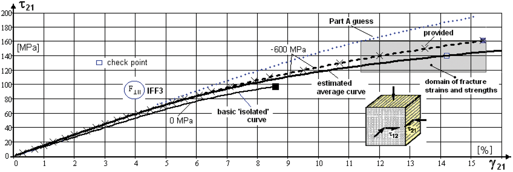$τ_{21} (γ_{21})$ for $σ_{hyd} = 0,^{} - 600$ MPa. UD T300 carbon/PR319 epoxy hoop wound tube. Properties, see TC2 and section 4.2. $τ_{21} \equiv τ_{out}$ . Part A curve: $b_{⊥ | |} = 0.3$ (dotted).

According to the obtained experimental data, the investigation of the TC2 through TC4 begins with the mapping of provided shear stress–shear strain data. The generated curve will be a single curve (≡ one test realisation) within the scatter band of the provided curves. For the envisaged strain-hardening FRP materials, this curve will be engineering-like mapped by

ɛ = σ / E_{0}^{\underline{m} od e} + 0.002 (σ / {\bar{R}}_{p 0.2}^{\underline{m} od e})^{n}

(8)

because the well-known MIL-Handbook 5 applies it as an engineering mapping tool, that is recognized in industry for this type of material behaviour. The R-O exponent

n = ℓ n (ɛ_{pl} (R_{m})) / ℓ n ({\bar{R}}_{m}^{\underline{m} od e} / {\bar{R}}_{p 0.2}^{\underline{m} od e})

(9)

is estimated from a strength point

({\bar{R}}_{m}^{\underline{m} od e}, ɛ_{pl} ({\bar{R}}_{m}^{\underline{m} od e}))

and a yield or, here, more as a quasi-yield point information. The description of the stress–strain curve requires 4 R-O parameters, where the ‘strength’ value

{\bar{R}}_{m} (p_{hyd})

is just one of them. Mapping needs the use of average properties. From the Part A information, a guess of this value could be obtained. Yield ‘strength’

{\bar{R}}_{c 0.2} (p_{hyd})

and the physically necessary

b_{⊥ | |} = 0.12

had to be estimated.

– The degree of the strain-hardening non-linearity mainly affects $E_{⊥}^{c}$ and $G_{| | ⊥}$ . It depends on the non-linearly behaving matrix material, the ‘2ndTg-shift effect’, and the finite strain-related ‘Birch effect.’¹⁴ The effect of 2ndTg would have caused that the fracture stress increases under $p_{hyd}$ is reduced and fracture shear strain is increased.

– Novel idea: There must be a link between TC2, TC3 (both the curves result from a bunch of different test specimen curves) and TC4 (single curve of the bunch). This link, marked by a common check point (hollow square) in the three figures, can be only obtained if the TC4 single curve is replaced by an average (typical) shear stress–shear strain curve.

For performing this, it is assumed that the centre of the ‘fracture stress/fracture strain domain’ is the most probable, ‘average’ failure point. The idea above to obtain an average curve is effortful, because all R-O parameters of each curve change, and no similarity can be stressed:

– Basic average ‘isolated’ curve, for orientation: $γ_{21} = τ_{21} / G_{| | ⊥} + 0.002 \cdot (τ_{21} / {\bar{R}}_{p 0.2, ⊥ | |})^{n}$ , constructed from provided UD data set and information from [Pae96]

\begin{matrix} n = 6.9, {\bar{R}}_{⊥ | |, 0.2} = 74 MPa, {\bar{R}}_{⊥ | |} = 97 MPa, \\ γ_{⊥ | |, fr} = 0.086, G_{| | ⊥} = 1330 MPa . \end{matrix}

Prediction of average $γ_{21} = τ_{21} / G_{⊥ | |}^{600} + 0.002 \cdot (τ_{21} / {\bar{τ}}_{21, 0.2}^{600, pred})^{n^{600}}$ on available data

– Estimation of a shear fracture value at $p_{hyd} = 600 MPa$ using the IFF3 equation:

\begin{matrix} {Eff}^{⊥ | |} = {[b_{⊥ | |} \cdot I_{23 - 5} \\ + (\sqrt{b_{⊥ | |}^{2} \cdot I_{23 - 5}^{2} + 4 \cdot {\bar{R}}_{⊥ | |}^{2} \cdot (0 + {\bar{τ}}_{21, fr}^{600, {pred}^{2}})^{2}}] \\ / (2 \cdot {\bar{R}}_{⊥ | |}^{3})}^{0.5} = 1 \end{matrix}

with

\begin{matrix} I_{23 - 5} = 2 \cdot σ_{2} \cdot (τ_{21, fr}^{600, pred})^{2} + 0 + 0, σ_{2} = - p_{hyd} \\ = - 600 MPa, b_{⊥ | |} = 0.3 \end{matrix}

obtaining

{\bar{τ}}_{21, fr}^{600, pred} (b_{⊥ | |} = 0.3) = 193 MPa

in Part A, instead of 137 MPa for

b_{⊥ | |} = 0.12

– Determination of remaining properties to compute the R-O parameters, estimated by using information from Pae-Shi curves¹⁵: $G_{⊥ | |}^{600} \approx 1.13 \cdot G_{⊥ | |} = 1503 MPa$ , $γ_{⊥ | |, fr}^{600} = 0.152$ , and the remaining needed R-O parameters could be estimated as $n^{600} = 5.5$ and ${\bar{τ}}_{21, 0.2}^{600, pred} = 125 MPa$ .

– Above data based on $b_{⊥ | |} = 0.12$ would practically lead to the Part B curve.

– Provided test data, single curve: $γ_{21} = τ_{21} / G_{⊥ | |}^{600} + 0.002 \cdot (τ_{21} / τ_{21, 0.2}^{600})^{n}$ ,

\begin{matrix} n = 3.8, τ_{21, 0.2}^{600} = 125 MPa, τ_{21, fr}^{600} = 161 MPa, \\ γ_{_{⊥ | |, fr}}^{600} = 0.154, G_{⊥ | |}^{600} = 1503 MPa \end{matrix}

– Searched Part B average (bar over) curve: $γ_{21} = τ_{21} / G_{⊥ | |}^{600, av} + 0.002 \cdot (τ_{21} / {\bar{τ}}_{⊥ | |, 0.2}^{600, av})^{n}$ ,

\begin{matrix} n = 4.6, {\bar{τ}}_{⊥ | |, 0.2}^{600, av} = 70 MPa, {\bar{τ}}_{⊥ | |}^{600, av} = 140 MPa, \\ γ_{_{⊥ | |, fr}}^{600, av} = 0.142, G_{⊥ | |}^{600, av} = 1503 MPa . \end{matrix}

Modifications from Part A to Part B: Change from estimated $b_{⊥ | |} = 0.3$ to 0.13 (Part B). Therefore, Part A showed a pretty blind prediction.

TC5: $σ_{2}^{fr}$ ( $σ_{3} = σ_{1})$ , UD E-glass/MY750epoxy (Figure 10)

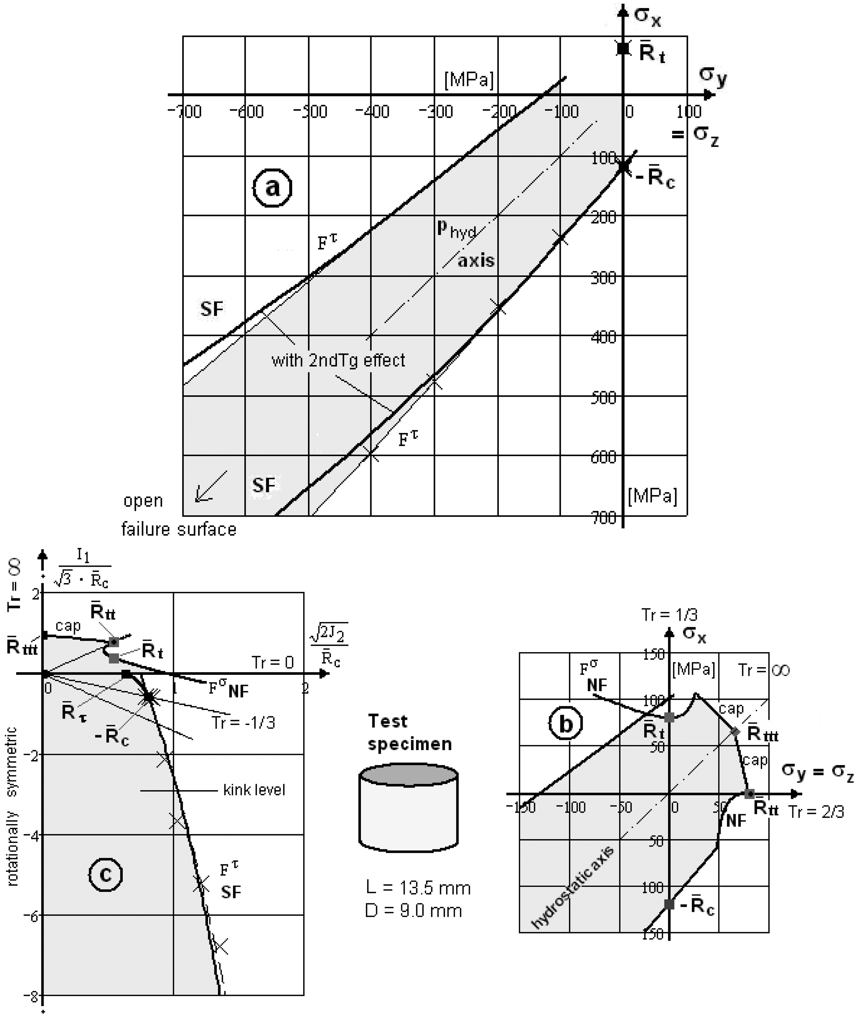
“Test data from Reference [ 10 ], compression tests: rectangular blocks (5 × 5 × 20 mm³ coupons, cut from filament wound UD panels) under combined axial loading with lateral pressure. During test, the (hydrostatic) pressure was first increased to a pre-determined level and then kept constant while $σ_{2}^{c}$ was increased continuously until the specimen fractured“.

Figure 10.

TC5: Tri-axial failure state of stress: 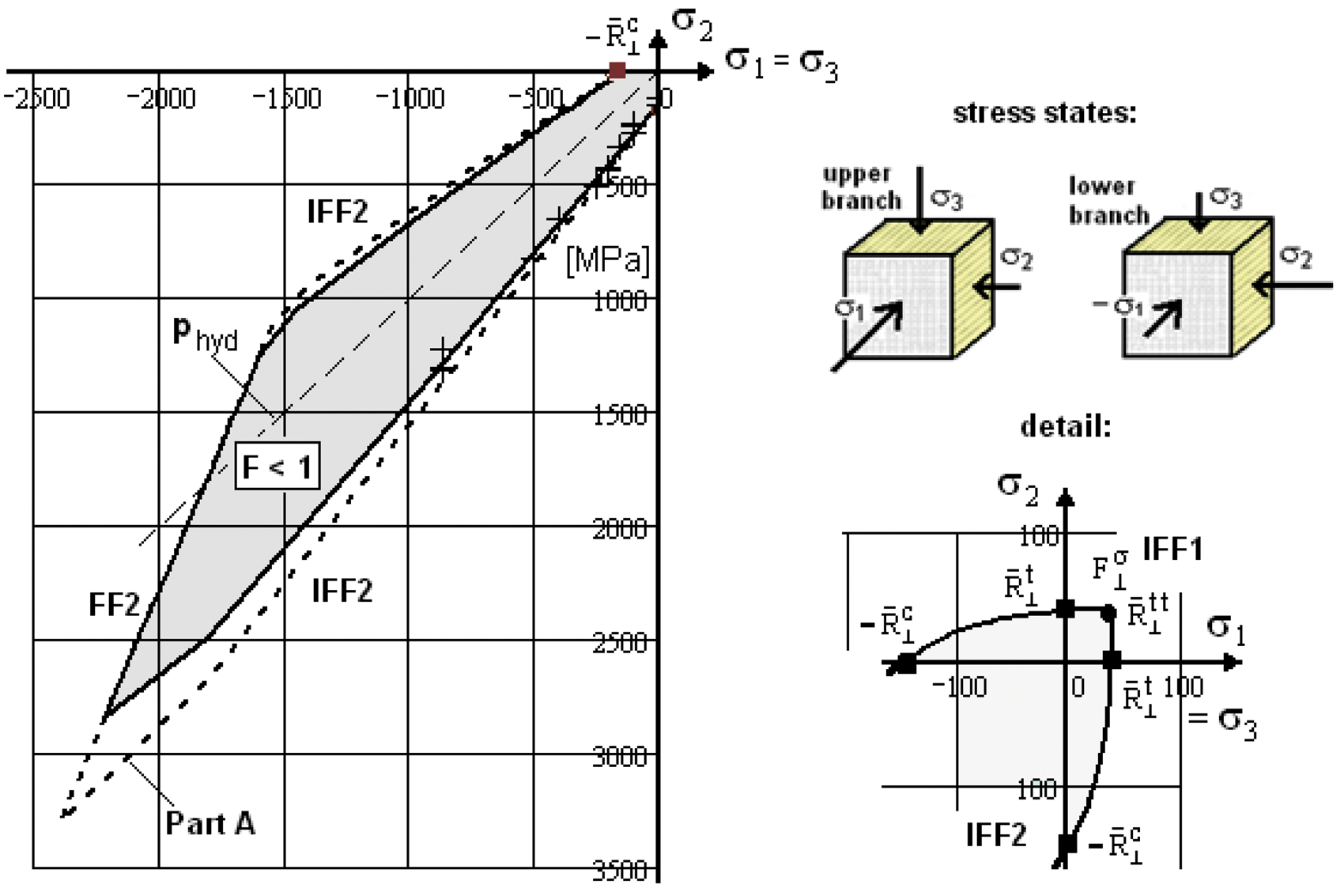$σ_{2}$ vs. longitudinal stress $σ_{1} (= σ_{3})$ for a UD E-glass/MY750epoxy cube. ${\bar{R}} = (1280,_{} 800,_{} 40,_{} 132,_{} 73)^{T} MPa$ . $ν_{⊥ | |} = 0.28$ , m = 2.8, $b_{⊥ ⊥} = 1.16$ , $ν_{m} = 0.35$ .

Task is the prediction of the failure envelope in all quadrants. Test data are provided for tri-axial compression in quadrant III, lower branch, only. They look good but do not indicate any 2ndTg effect by a kink point or deflection point, respectively. A comparison can be only made in quadrant III.

– The slope of the course of test data shows that the UD material is less brittle than assumed in Part A. Therefore, the friction parameter $b_{⊥ ⊥} = 1.21$ , estimated in Part A, was lowered to 1.16. As lateral strength, the Part A value ${\bar{R}}_{⊥}^{c} = 145 MPa$ is to be kept (organizers) despite of the fact that in case of mapping an average value of the three Part B-provided compressive test data of 132 MPa should have been taken. This has an effect on well mapping the test data.

Modifications from Part A to Part B: Change $b_{⊥ ⊥} = 1.21 \to 1.16$ , $b_{⊥ | |} \equiv μ_{⊥ | |} = 0.3 \to 0.2$ . Part A curve would coincide with Part B if friction parameters could have been provided for Part A.

TC6: $σ_{1, fr} (σ_{3} = σ_{2})$ , UD S-glass/epoxy (Figure 11)

“The test data were taken from Zinoviev and from Wronski and Parry Reference [ 16 ]”.

Figure 11.

TC6: Through-thickness stress 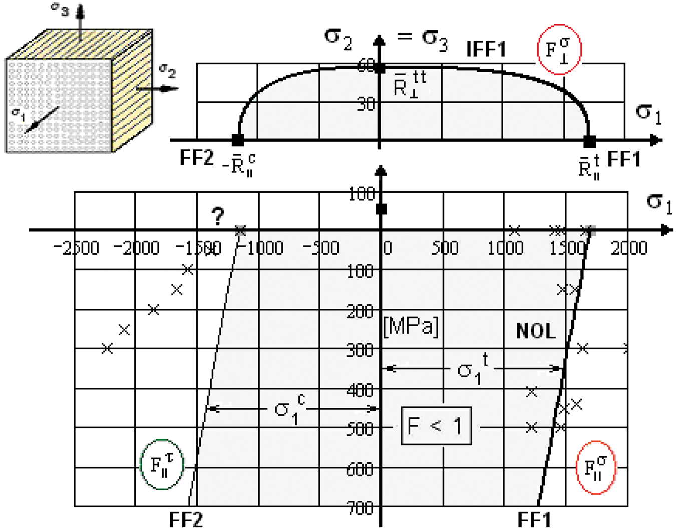$σ_{3} (= σ_{2})$ vs. fibre-parallel stress $σ_{1}$ , UD S2-glass/epoxy waisted test specimen. ${\bar{R}} = (1990,_{} 1500,_{} 38,_{} 150,_{} 70)^{T} MPa$ , $ν_{⊥ | |} = 0.3$ , m = 2.8, $b_{⊥ ⊥} = 1.21$ , $b_{⊥ | |} = 0.13$ .

The test data of TC6 and TC7 show large differences in quadrant IV. For mapping of the tension curve FF1 in quadrant IV no reliable test data set was provided. TC 6 presents a diffuse scatter in quadrant IV. This can be explained from own tests with Naval Ordinance Laboratory (NOL) rings. It is known that the additional bending stress at tensioning the NOL ring causes pretty a stochastic fracture with a fracture level pretty lower than that from the usual coupon test. A stadium ring would have delivered better results but is more difficult to produce. Therefore, the results from Zinoviev cannot be used for validation.

– The tendency of the left branch, mode FF2, from Wronski-Parry (quadrant III) is the same as in TC7, fortunately, and could be a validation basis. The left branch indicates a kink and thereby – for the first time possibly – seems to indicate some 2ndTg-effect.

– In TC3 and TC4, it was demonstrated that the shear fracture strain increases with $p_{hyd}$ . This will also occur in the case of tensile fracture strain due to the beneficial acting (healing) of $p_{hyd}$ . However, it is to be sorted out which portion belongs to the Poisson effect (governed by $ν_{⊥ | |}$ ) and which portion to a healing effect. The author predicted the almost linear increase of the compressive fracture stress with $p_{hyd}$ in a test case cited in Reference [17] by employing just the Poisson effect, which always causes tensile pre-straining. Incomprehensible, this was not successful in the case of TC6 and TC7.

– TC7 will be the better test case for deeper investigations than TC6 and shall be discussed. Just the fibre material is different, glass changes to carbon.

Modifications from Part A to Part B: None.

TC7: $σ_{1, fr} (σ_{3} = σ_{2})$ , UD A-S/epoxy (Figure 12)

“Test data from Parry-Wronski. ¹⁸ ¹⁹ Tests executed with dog-bone test specimens, as before. Failure modes observed are longitudinal splitting, kinking, kink band”.

Figure 12.

TC7: Through-thickness stress 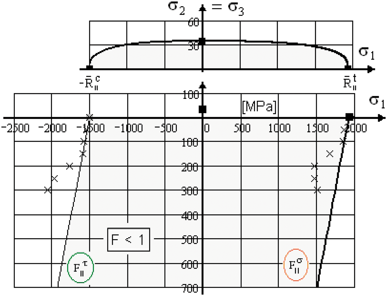$σ_{3} (= σ_{2})$ vs. fibre-parallel stress σ₁. UD A-S carbon/epoxy1. ${\bar{R}} = (1990,_{} 1500,_{} 38,_{} 150,_{} 70)^{T} MPa$ , $ν_{⊥ | |} = 0.3$ , $m = 2.8$ .

The course of the test data indicates that the predictions in Part A may have been performed on the basis of a not really understood 2ndTg matrix modelling and that the matrix does not really show any 2ndTg-effect. On top, still now, some discrepancies disturb the use of the provided TC7 test data for model validation.

Due to missing test points, the provided through-thickness strength ${\bar{R}}_{z} = 38 MPa$ will not be used. Data of the Part A UD model will be used further and it will not be moved to an orthotropic model.

– Test data look better than in TC6. However, it is not understood why the tendency of the curves in quadrant III and IV is so different. Primarily, Poisson is acting at smaller bi-axial states of compression stresses first, the 2ndTg effect acts later at higher pressures. Therefore, due to the Poisson effect, the compressive fracture failure strain and similarly the failure stress in quadrant III, which acts at the cross section, is increased and in quadrant IV the tensile failure strain (right curve) is reduced. This would result in a similar curvature tendency in both the quadrants.

With increasing failure strain, the ‘compression’ curve becomes more horizontal and the ‘tension’ curve more vertical. How long the vertical drop will go (the provided data set ends at $σ_{2} = σ_{3} = - 300 MPa$ ) is not demonstrated. In contrast, note that it is proven in Reference [10], that the tensile fracture stress will reduce with $p_{hyd}$ till $- 860 MPa$ and this is in the sense of an acting Poisson effect.

– In quadrant IV, it looks at $- 150 MPa$ either as if the fracture strain is reduced or as if the Poisson effect would have doubled. Below the bi-axial compression level of $σ_{2} = σ_{3} = - 300 MPa$ , the Poisson effect ‘vanishes’ and the tensile stress, acting at the cross section, keeps the same value of about $1500 MPa$ . In other words, the fracture strain of the filament would increase. Usually, the 2ndTg-effected matrix reduces stiffness and this would increase the Poisson effect and cause the opposite curvature or tendency of the provided data curve. It would become flatter instead of steeper or even vertical. Also, if the interphase between filament and matrix breaks then the bi-axial pressure will cause an elongation of the filament linked to its Poisson’s ratio $ν_{f}$ which is not so much different to the UD value $ν_{12}$ .

– All the courses of the provided test data and of other test data have a flattening tendency as it is also depicted in quadrant III. From this might be questioned whether measurement or evaluation of the provided test data might not be adequately performed, at least in quadrant IV. Influence on the curves have the in-plane major Poisson’s ratio $ν_{12}$ (the smaller $ν_{12}$ , the steeper the curve), the ‘healing’ effect from bi-axial compression (may increase failure strain) and from the 2ndTg-effect. The author is not able to physically explain the discrepancies.

Modifications from Part A to Part B: None.

TC8: $σ_{y, fr} (σ_{z} = σ_{x})$ , E-glass/MY750epoxy, laminate [35/-35/]_ns (Figure 13)

“The test data were taken from Reference [ 20 ] and the test specimens were filament wound tubes”.

Figure 13.

TC8: Effect of the applied surface pressure 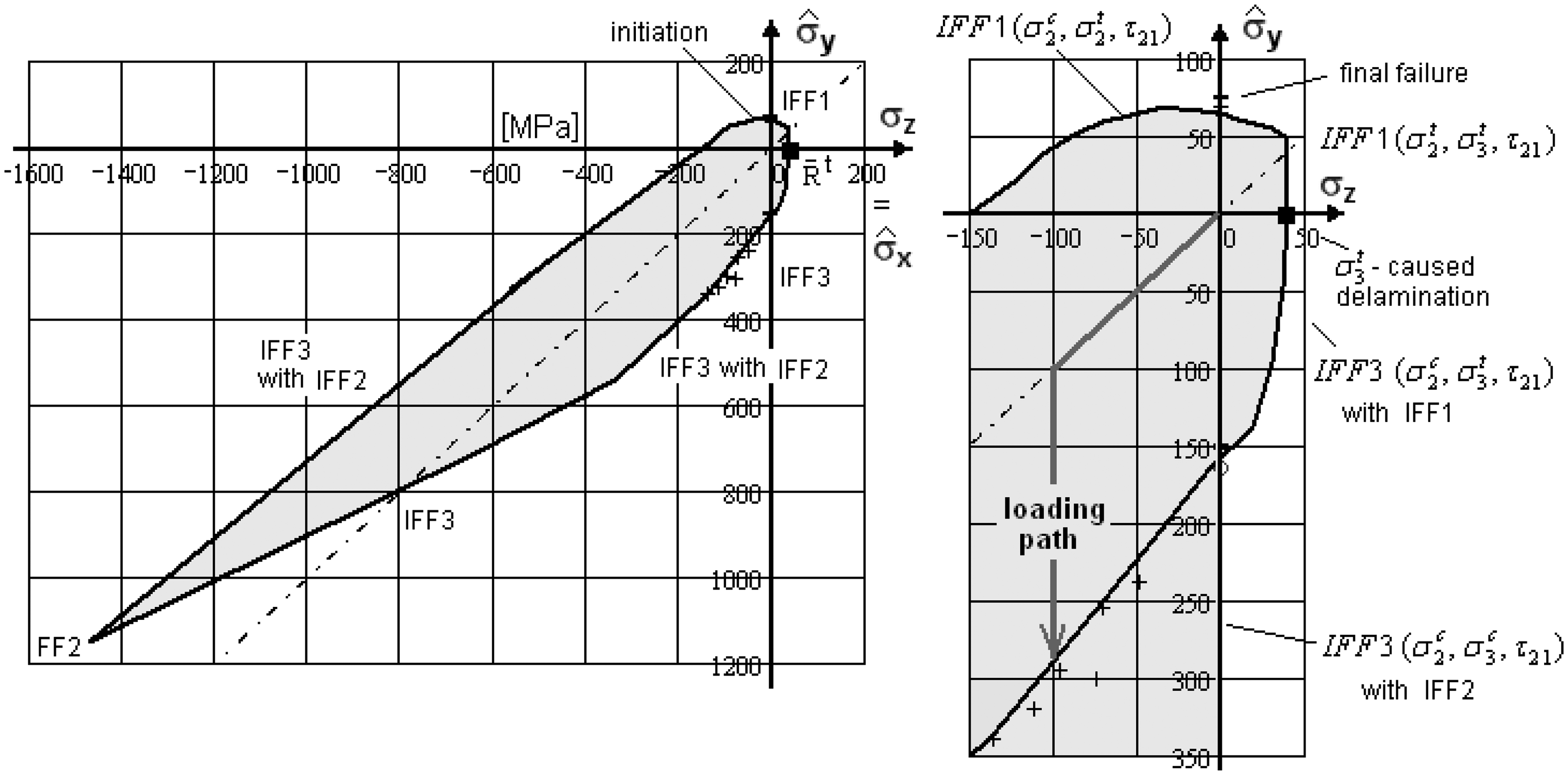$σ_{z} = - p$ (through-thickness stress) on the size of the normal section force $n_{y} = {\overset{\land}{σ}}_{y} / t$ at fracture, with $n_{x} / t = {\overset{\land}{σ}}_{x} = σ_{z}$ . Thick-walled tube, UD lamina-composed laminate [35/–35/35/–35], E-glass/MY750/epoxy. Properties and stress states, see TC5. Loading path respecting computation is indicated.

Data for the upper branch is missing. Data for the quadrants I, II, IV could be not provided in order to have a good basis for the validation. Figure 14 describes test arrangement and stresses. The high values of the three test data at the positive ${\overset{\land}{σ}}_{y}$ -axis cannot be explained by the author.

– A re-investigation of the friction parameter $b_{⊥ ⊥} = 1.21$ by some curve ‘data fitting’ showed that it had to be reduced to 1.16 as for TC5. This value is substantiated by information from WWFE-I. The other friction parameter $b_{⊥ | |} \equiv μ_{⊥ | |}$ is obtained by mapping the test data provided for quadrant III. Note that TC5, TC8 and TC9 possess the same material (see table 2 in Part A) but belong to different test specimens, which will naturally cause some difference in ‘strengths’.

– An improved non-linear programming is necessary, especially due to the fact that in TC9 both the failure modes IFF2 and IFF3 have a similar risk to fracture, or - in other words - the material stressing effort is similar for both modes in the envisaged two-fold failure domain.

– The fibre volume contents for Part B was increased from the initial 60% up to $V_{f} = 67 %$ (‘dry’ filaments possible) This would make a correction necessary so that the TC8 data do not remain the same as for TC5, but, the driving strengths in the compression domain ${\bar{R}}_{| |}^{c}, {\bar{R}}_{⊥}^{c} . {\bar{R}}_{⊥ | |}$ might not become better. Therefore, the values for ${\bar{R}}_{| |}^{c}, {\bar{R}}_{⊥}^{c}$ are kept.

Figure 14.

Modelling of TC8 test situation, t_k = 0.25 mm, t = 2 mm laminate thickness.

An increase of the fibre volume content on the elasticity properties is not considered due to the other uncertainties and that the stress–strain curve would have to be adapted and hardening parameters to be reworked with all its work consequences.

Modifications from Part A to Part B: Change of $b_{⊥ ⊥} = 1.21 \to 1.16$ , $b_{⊥ | |} \equiv μ_{⊥ | |} = 0.3 \to 0.2$ . With the Part B knowledge the same curve would have been obtained for Part A, too.

TC9: $σ_{y, fr} (σ_{x} = σ_{z} = - 100 MPa)$ , properties. see TC8 (Figure 15)

Figure 15.

TC9: Comparison between theoretical predicted stress–strain curves 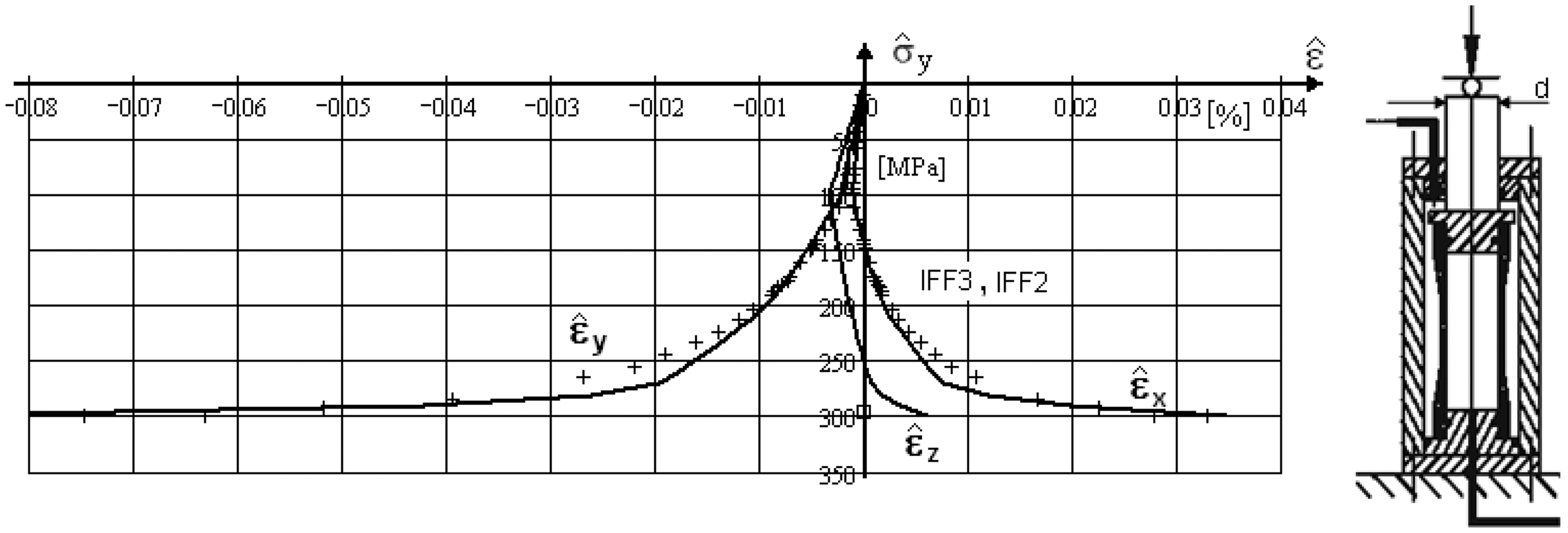${\overset{\land}{σ}}_{y} ({\overset{\land}{ɛ}}_{x})$ and ${\overset{\land}{σ}}_{y} ({\overset{\land}{ɛ}}_{y})$ and experimental data for a [35/–35/35/–35] _s E-glass/MY750 epoxy laminate. Solid curves are predicted curves; measured data (+) taken from Reference [9]. Properties and loading, see TC8. Monotonically loaded ${\overset{\land}{σ}}_{x} = {\overset{\land}{σ}}_{y} = σ_{z}$ up to −100 MPa, then ${\overset{\land}{σ}}_{y} = n_{y} / t$ grows further.

“Test data were taken from Reference [ 20 ].”

Data for $ɛ_{z}$ are missing. The final state of stress does not show a 2ndTg-effect.

Modifications from Part A to Part B: Change of $b_{⊥ ⊥} = 1.21 \to 1.16$ , $b_{⊥ | |} \equiv μ_{⊥ | |} = 0.3 \to 0.2$ .

TC10: $τ_{yz, fr} (σ_{z} = σ_{x})$ , IM7/8551-7, quasi-isotropic laminate [45/-45/90/0]_ns (Figure 16)

Figure 16.

TC10: Applied section shear load-caused maximum-thickness failure shear stress 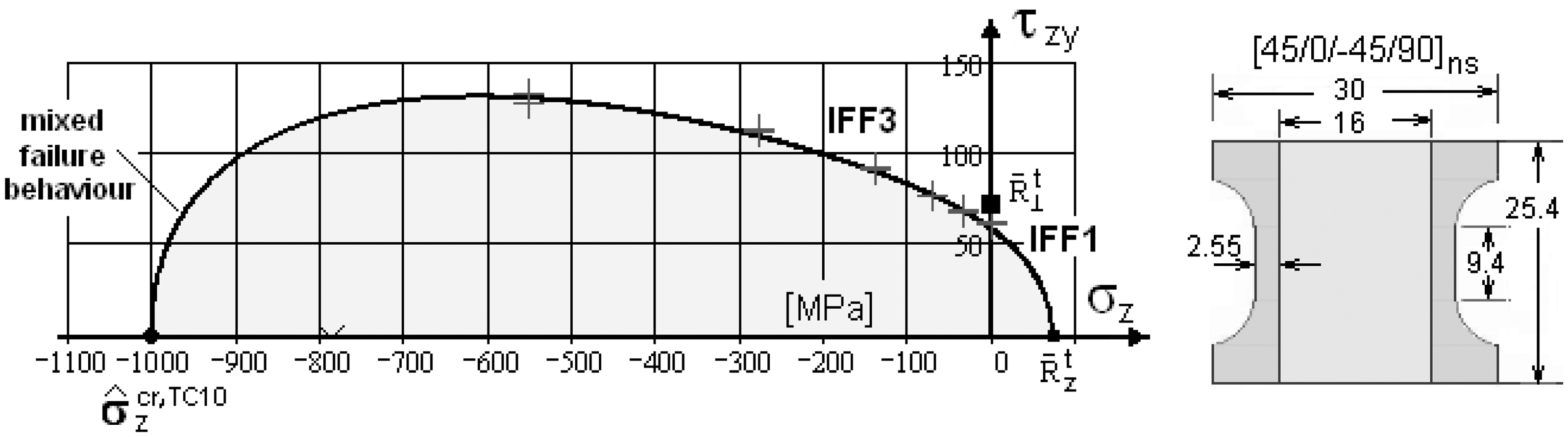$τ_{zy}$ vs. applied through-thickness stress $σ_{z}$ for a [45/0/–45/90]_ns, carbon/epoxy laminate, IM7/8551-7. $r_{inn} = 7.95 mm$ , $t = 2.55 mm,$ $t_{k} = 0.25 mm$ , $ν_{⊥ | |} = 0.34$ , ${\bar{R}} = (2560,_{} 1590,_{} 73,_{} 185,_{} 90)^{T} MPa$ , ${e_{fr}} = (1.55,_{} 1.1,_{} 0.87,_{} 3.2,_{} 5)^{T} %$ , $E_{| |} = 165000 MPa$ , $E_{⊥} = 8400 MPa$ , $G_{| | ⊥} = 5600 MPa$ ; $R_{z}^{t} = 63 MPa$ . $b_{⊥ ⊥} =_{} 1.2$ , $b_{⊥ | |} = 0.25$ , ${\overset{\land}{σ}}_{z}^{squ, TC 10} = - 1000 MPa$ , $m = 2.2$ . Provided test data: +, x.

“Test data were taken from DeTeresa.²¹ ²²

Figure 17(a) shows a 90°-lamina of the stack of the thick-walled tube milled from a laminate block. For comparison, Figure 17 depicts the traditional wound or tape-layered tube; $r_{inn} = 7.95 mm$ , $t = 2.55 mm,$ $t_{k} = 0.25 mm$ . In TC10 and TC11, short hollow waisted test specimens are used. For such a specimen, termed ‘cylindrical’ in Reference [23], an average strength of $\overset{\land}{\bar{}} σ_{z}^{cr} = - 783 MPa$ (5 tests) was measured. However, for the quasi-isotropic (not cross-ply, as TC 12 is marked!) solid waisted specimen (5 tests) of TC12 $\overset{\land}{\bar{}} σ_{z}^{cr} = - 1363 MPa$ was obtained. From the difference it can be learned that hollow specimens fracture much earlier due to structural instability failure which is triggered by the previous material damaging. Therefore, for the quasi-isotropic TC10 tube (angle-ply) and the waisted cross-ply tube TC11, the average ‘solid’ crushing strength $\overset{\land}{\bar{}} σ_{z}^{cr} = - 1363 MPa$ must be reduced for the prediction of the curve in the high compressive domain. Hence, the recommendation of the reviewer, to use $\overset{\land}{\bar{}} σ_{z}^{cr} = - 1363 MPa$ for TC10 and for 11, cannot be followed. For TC10, as through-thickness compressive fracture stress (crushing strength) $\overset{\land}{\bar{}} σ_{z}^{cr, TC 10} = - 1000 MPa$ is used as compromise.

Figure 17.

Modelling of TC10 test situation: (a) a 90°-lamina of the stacked thick-walled tube milled from the sketched laminate block for comparison and (b) the traditional wound or tape-layered tube.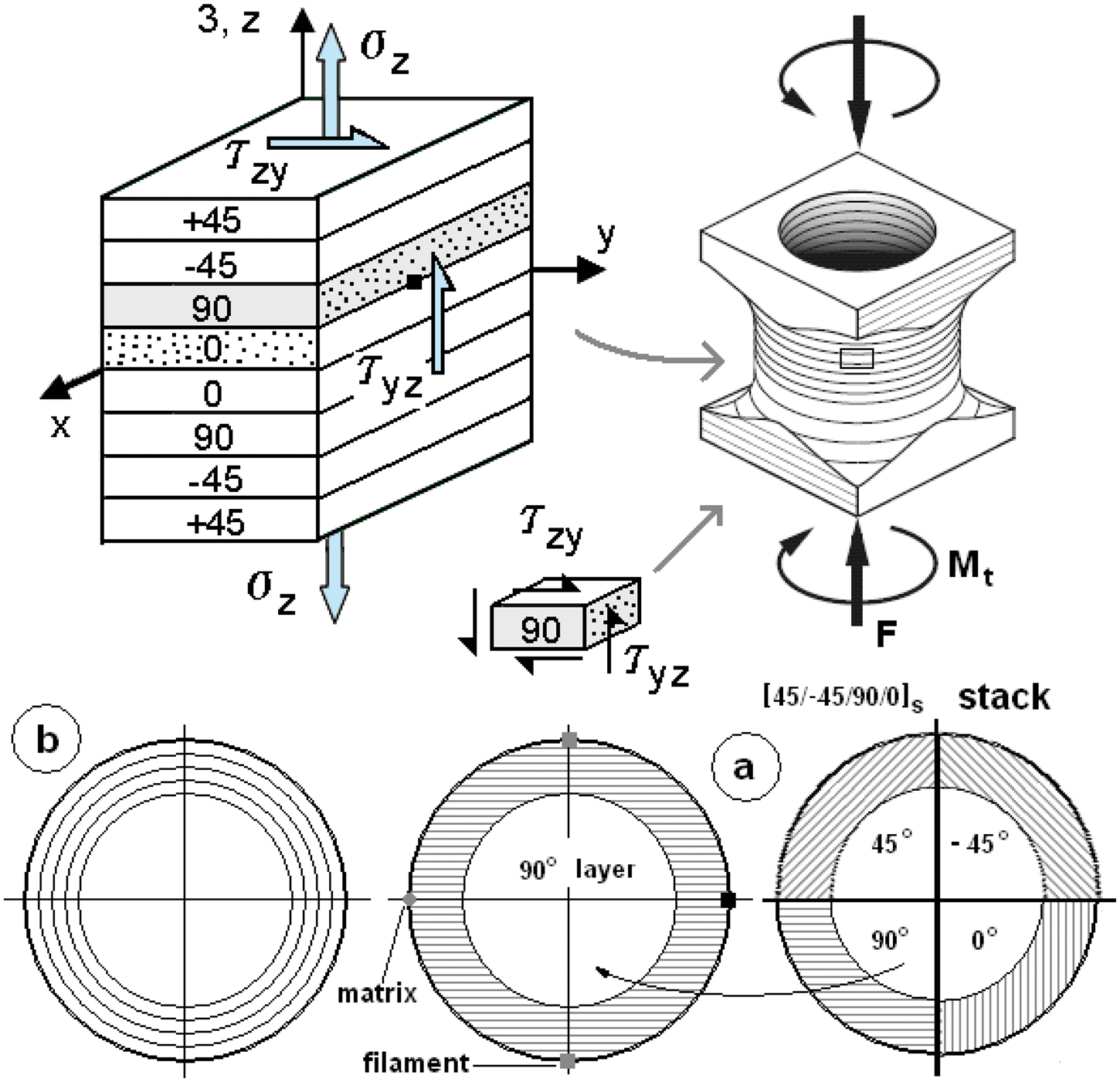

Test situation does neither generate a uniform stress state in the critical locations nor a small stress gradient. With respect to the non-uniform shear stress field at the cross-section plane, it can be stated that the test specimen does not give much experimental evidence. The specimen encounters multi-site failure within each lamina and at the same time multi-ply failure in all laminas. This means that a multi-fold fracture danger is given in the stack. Therefore, the specimen is not an adequate tool to validate strength-failure conditions.

In Figure 17, maximum filament and matrix failure locations are indicated. These critical locations are bound to the varying lamina fibre orientation and take different positions over the stack and can be assumed. The failure mode is IFF and the associated critical interlaminar stress state can be estimated.

Three different sub-stack descriptions are found in the provided documents: [45/–45/90/0]_ns, [90/45/–45/0] and [45/0/–45/90] (from theoretical reasons a stack with minimum angle change would be best because it leads to the smaller interlaminar stresses to achieve compatibility of the lamina deformations). However, this does not have an effect because the specimen is milled from a laminate brick.

– The tube is thick-walled, which means that the outer shear stress will be fracture decisive. Principally, for TC 10 and TC11, a lamina-to-lamina 3D FEA would be necessary for stress analysis. In Reference [13], a ‘smeared’ model is presented that substitutes the effortful 3D model. This helps to obtain a faster solution for the specimen’s deformation behaviour. Finally however, the actual stress state at the critical location is required for strength judgement.

– Before using the provided approximate quasi-isotropic laminate's through-thickness (crushing or squeezing) fracture stress value ${\overset{\land}{σ}}_{z}^{cr}$ of the (structure) laminate in the (material) strength failure condition, it should be thought how far the type of fracture might remain material failure. For instance, if filaments of the stacked layers come to lie upon another, this leads to a failure which is not covered anymore by a material strength failure condition. It is obvious that crushing of a laminate is the “end” of further operational use. The crushing stress value is the consequence of several effects: micro-cracking, FF1, filament-upon-filament, edge effects and structural instability. This means: A material failure condition can only partly predict this mixed failure phenomenon.

Modifications from Part A to Part B: TC10 was not investigated in Part A. A test curve is the result of both the partners, of test specimen and of test rig. In Part A, the author assumed an ARCAN test rig, loaded by scissor forces F , whereas in Part B the De Teresa torque test rig is used. This caused a change in the prediction of failure location as well of type and curve. The ARCAN test rig shows a more uniform stress state than the DeTeresa torque test rig.

TC11: $τ_{yz, fr} (σ_{z} = σ_{x})$ , IM7/8551-7, cross-ply laminate [0/90]_ns (Figure 18)

“Test data from De Teresa, ¹² ^, ¹³ test execution as for TC10”.

Figure 18.

TC11: Thickness failure shear stress 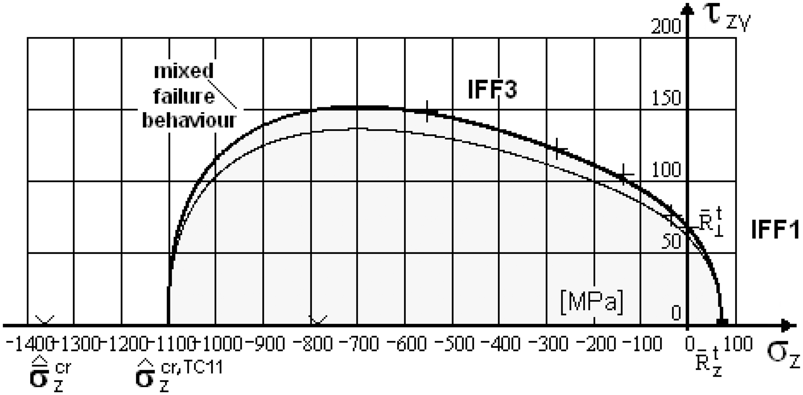$τ_{zy}$ vs. applied through-thickness stress $σ_{z} = - p$ for a [0/90/0/90]_ns. Properties, see TC10; ${\overset{\land}{σ}}_{z}^{cr, TC 11} = - 1100 MPa$ (assumed). Lower curve is basic model.

The dog-bone-shaped tube test specimen TC11 has less different layer angles than TC10. Therefore, the fracture curve should be longer and lie a little higher than curve TC10 due to the fact that a lower number of critical locations (just 0° and 90°) is encountered. This fracture stress capacity, higher than for TC10, is assumed to be $\overset{\land}{\bar{}} σ_{z}^{cr,^{} TC 11} = - 1100 MPa$ . Again, the solid block specimen of TC12 exhibits higher ‘strength’ than the TC11 tube.

Modifications from Part A to Part B: The test rig became known and the loading situation had to be fully reworked. The assumed crushing stress was increased from ${\overset{\land}{σ}}_{z}^{cr, TC 11} = - 780 MPa$ in Part A (used as minimum value of three points, safe side) down to $- 1100 MPa$ .

TC12: ${\overset{\land}{ɛ}}_{x} (σ_{z}^{c}) = {\overset{\land}{ɛ}}_{y} (σ_{z}^{z}), ɛ_{z} (σ_{z}^{z});$ IM7/8551-7, [0/90/0/90]_ns (Figure 19)

“No data was available from the work reported by DeTeresa et al. for this Test Case. Consequently, the organisers suggest experimental data that could be used a guidance illustrating the likely response of similar laminates (quasi-isotropic [45/0/–45/90]_ns) under through-thickness compression of solid waisted specimens, obtained by Kaddour et al.” ²⁰

Figure 19.

TC12: Predicted single stress–strain curve caused by a through-thickness compressive stress 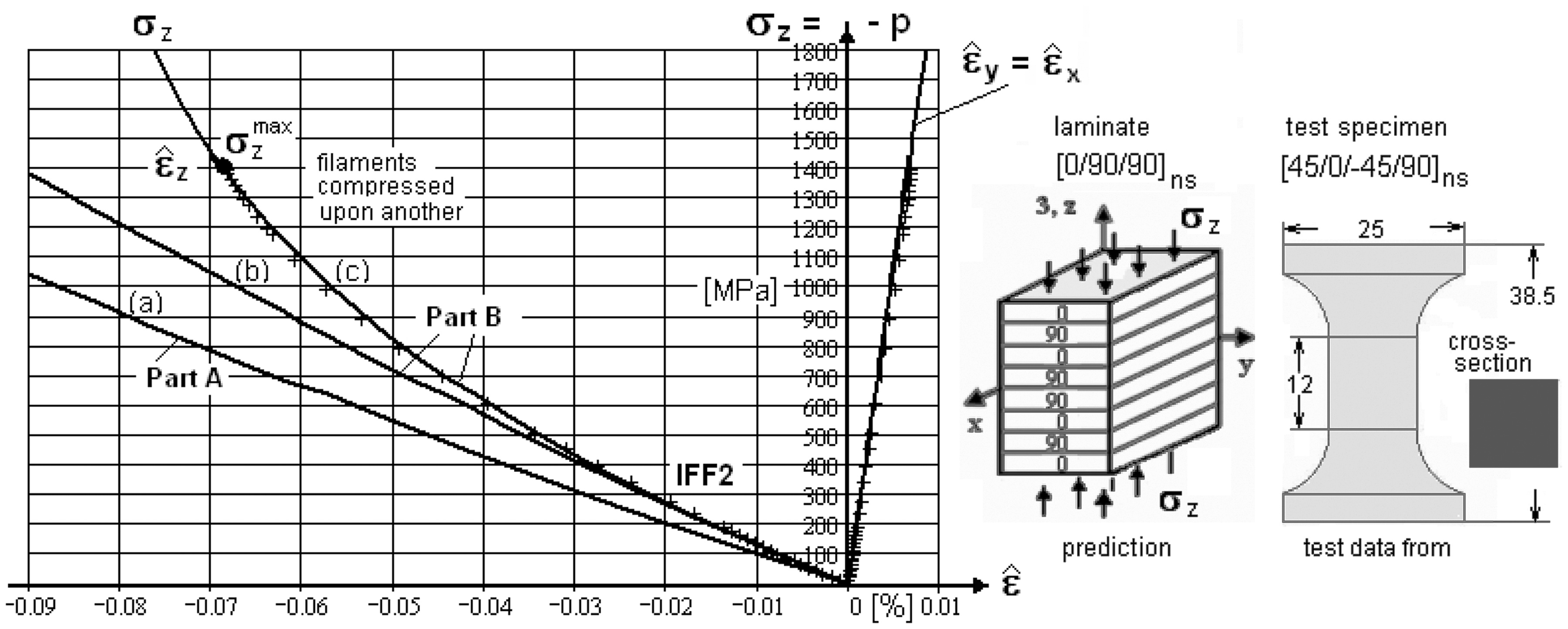$σ_{z} = - p$ for a [0/90/0/90]_ns versus test data (+) from a quasi-isotropic laminate [45/0/–45/90]_ns, $σ_{x} = σ_{y} = 0$ . Curves: (a) Part A after sign correction, $E_{⊥} = 8400 MPa$ ; (b) Part B, $E_{⊥} = 11000 MPa$ and (c) Part B, $E_{⊥} = 11000 MPa$ and with equation (10).

It is not clear why this TC is marked as a cross-ply, but the curve stems from a lay-up that is a quasi-isotropic angle-ply! The effect of the curing stress is of practical interest in the positive domain, and therefore not requested in quadrant III.

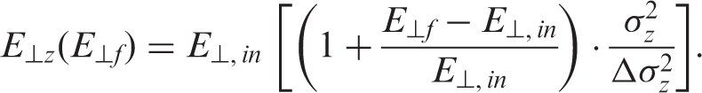
– The provided (in Part B) similar curve will be considered. It is one single curve of 5 experiments. The through-thickness stress $σ_{z}^{max} = - 1400 MPa ≅ \overset{\land}{\bar{}} σ_{z}^{cr} = 1363 MPa$ (average of the 5 tests) is not marked as final fracture, however, it may be final fracture from operational reasons assumed as the practical final fracture. In this context: The tube specimens in TC10 and TC11 finally show a structural failure, the TC12 waisted specimen not. TC12 experiences lateral material crushing.

– The Part A curve does not have the tangent stiffness of the ‘similar’ curve. Because a 3D-CLT delivered the same low initial slope, it could be concluded that the transverse elasticity moduli $E_{⊥, in}$ of Part A and B do not correspond, and the provided elasticity modulus in thickness direction is too low and to be increased.

– A further effect is to be considered: With increasing thickness reduction, the filaments are more and more pressed upon another. By that, the composite modulus $E_{⊥ z}$ approaches $E_{⊥ f} = 19000 MPa$ . To achieve this, the “similar” curve is to be mapped applying a simple quadratic approach ( $Δ σ_{z} = - 1700 MPa$ , $E_{⊥, in} = 11000 MPa$ ) through $σ_{z}^{max}$ and the origin:

E_{⊥ z} (E_{⊥ f}) = E_{⊥, in} [(1 + \frac{E_{⊥ f} - E_{⊥, in}}{E_{⊥, in}}) \cdot \frac{σ_{z}^{2}}{Δ σ_{z}^{2}}] .

(10)

Modifications from Part A to Part B: (1) Correction of a mistake (curvature of the predicted curve in Part A was opposite to the experimental curve. Caused by a typing error in the equations coded). (2) Increase of the initial lateral elasticity modulus at origin from $E_{⊥, in} = 8400 MPa$ (Part A) to 11000 MPa (Part B). (3) Consideration of a growing filament contact by a stiffness increase model.

Comparison between theoretical predictions and experiments

Some additional figures are added to demonstrate special features of modelling and tests.

TC1: Matrix MY 750, ${σ} = (σ_{x}, σ_{y} = σ_{z}, σ_{z}, 0, 0, 0)^{T} \equiv (σ_{I}, σ_{II}, σ_{III})^{T}$

Problem: How does tri-axial compression influence the failure behaviour if two components of the stress vector are equal?

Task: Determination of the tri-axial fracture failure curve $σ_{x, fr} (σ_{y} = σ_{z})$ , Figure TC1 and validation of the 2ndTg model of the matrix to capture the 2ndTg-effect on the matrix.

It is well known from the cited literature and at QinetiQ that hydrostatic pressure stress states higher than 200 MPa will change the second glass temperature point of the matrix with the described stiffness worsening effect on the matrix. Second Tg-effect and Birch-effect have been effortfully implemented into the author's FMC-based 3D-CLT-MathCad program.

Comparison:

– Figure 5(a): Mapping of provided test data in quadrant III with provided data (thin) and with an assumed 2ndTg shift effect (bold) to show tendency in the case of the assumed effect size would occur. The slope of the lower curve with the assumed 2ndTg-effect shows a reduction beyond −300 MPa. This means that the compressive stresses $σ_{y} = σ_{z}$ have to be increased to carry the same load as without matrix weakening. A 10% slope decay starting at the kink point was considered between 200 and 600 MPa.

– Figure 5(b) predicted curves in the quadrants I, II, IV: An interaction of shear failure (SF) and normal failure (NF) in their transition zones in the quadrants II and III (Figure 5(b)) by a simple linear approach in 3D space (Figure 5(c)), characterized by Lode coordinates, was not executed due to a lack of data in the transition zones.

– Figure 5(c): Visualisation of provided test data in 3D space with provided data (dashed) and with an assumed 2ndTg shift effect (bold).

– Mapping of test data, given in quadrant III only, could be achieved after describing shear failure in a more ductile way (due to Part B information). This meant, lowering the unknown friction parameter from $b_{τ}^{c} = 1.52$ (brittle) in Part A to 0.18. In this context, one should recall that 0.18 almost reflects ductile behaviour and $b_{τ}^{c} = 0$ means ‘Mises yield cylinder’.

Results: (1) A 2ndTg-effect seems not to exist for the matrix. Unfortunately, 2ndTg modelling – needed for the following TCs – could not be substantiated by the provided matrix test data set. (2) Course of given data could be well mapped. In Figure 5(b) and TC1(c), the interaction or out-smoothing in the transition zones SF-NF was not performed. Failure surface is not closed.

TC2: UD lamina T300/PR319, ${σ} = (σ_{1}, σ_{2}, σ_{3} 0, 0, τ_{21})^{T}$

Problem: Influence of hydrostatic pressure $p_{hyd}$ on the in-plane fracture shear stress.

Task: Determination of the fracture failure curve $τ_{21, fr} (p_{hyd})$ with $σ_{1} = σ_{2} = σ_{3} = - p_{hyd}$ , and $p_{hyd}$ as an absolute pressure value, Figure 6.

Comparison:

– Course of scattering 90° tube test data could be well mapped after considering the average stress–strain curve and the hoop stress distribution (outer hoop stress is higher than the inner one).

– The sudden increase (jump) at zero hydrostatic pressure is assumed to be the consequence of the healing by $p_{hyd}$ and was modelled by the simple approach mentioned. Then, the full course of the correlated test points could be excellently mapped. ‘Check point’ for TC2 through TC4 is the open square in the three figures. It serves as verification of the approach.

– The failure curve is closed (still shown in Part A). But, to add to the Figures TC2 and TC3, an estimated closed failure curve is speculative and adds no value to the comparison because the failure is no material failure anymore but very likely structural failure that cannot be predicted by a strength failure condition for that material.

TC3: UD lamina T300/PR319, ${σ} = (- p_{hyd}, σ_{2} = - p_{hyd}, - p_{hyd}, 0, 0, τ_{21})^{T}$

Problem: Influence of the hydrostatic pressure $p_{hyd}$ on the in-plane fracture shear strain.

Task: Determination of the fracture failure curve $γ_{21} (σ_{2}^{fr}, τ_{21}^{fr})$ , Figure 7.

Comparison:

– Course of scattering 90° test data could be well mapped. The failure curve is closed.

– The sudden increase (jump) at zero hydrostatic pressure is assumed to be the consequence of the healing influence of $p_{hyd}$ and was modelled in the above simple way.

TC4: UD lamina T300/PR319, ${σ} = (- p_{hyd}, σ_{2} = - p_{hyd}, - p_{hyd}, 0, 0, τ_{21})^{T}$

Problem: Influence of an initially constant hydrostatic pressure on the in-plane shear stress–shear strain curve.

Task: Determination of the stress–strain curve $τ_{21} (γ_{21}^{fr})$ for $p_{hyd} = 600 MPa$ . Hereby, the shear is superimposed on the still acting $p_{hyd}$ .

Comparison:

– The determination of an average curve (bold) enabled to equally well map TC2 and TC3 and to show up the check point that links the curves.

– The provided single curve test data could be well mapped (dashed curve in TC4).

Note: The ‘check point’ ( $γ_{21} = 0.142, τ_{21} = 140 MPa, p_{hyd} = 600 MPa$ ) was intentionally not further ‘optimized’ with respect to the necessary iterations between the three TCs.

TC5: UD lamina E-glass/MY750 Epoxy, ${σ} = (σ_{1} = σ_{3},_{} σ_{2},_{} σ_{3},_{} 0,_{} 0,_{} 0)^{T}$

Basic problem: How much lateral stress $σ_{2}$ can the UD material sustain if a fibre-parallel stress $σ_{1}$ acts which is equal to a through-thickness stress $σ_{3}$ ? Test practice: $p_{hyd}$ is superimposed by a lateral compressive stress $σ_{2}^{c}$ at the $σ_{2}$ -surfaces. $σ_{1}$ is the stress acting at the respective coupon surface; the diagonal is the $p_{hyd} - line$ .

Task: Determination of the fracture failure curve $σ_{2, fr} (σ_{1} = σ_{3})$ in the quadrants III and IV.

Comparison:

– The course of provided test data could be well mapped. The failure curve is closed.

– Assuming that the model pre-requisites remain valid, final failure by kinking (FF2) is possible under $p_{hyd}$ (see TC2 in section 4.3 and Part A, Figure TC5), according to the following relationship $E_{| |} \cdot ɛ_{1} = - p_{hyd} \cdot (1 - 2 \cdot ν_{12})$ with $ν_{12}$ as larger Poisson’s ratio.

– Computation indicates wedge failure IFF2 in quadrant III. Under $σ_{3}^{t}$ , IFF1 is final failure.

– For information: Test data from DeTeresa²⁴ for the upper branch (2nd solution) of the failure curve in quadrant III are lying on the predicted upper branch after being re-evaluated by subtracting $p_{hyd}$ .

TC6 : UD lamina S-glass/epoxy, ${σ} = (σ_{1}, σ_{2}, σ_{3} = σ_{2}, 0, 0, 0)^{T}$

Problem: How much compressive fibre-parallel stress $σ_{1}^{c}$ can the UD material sustain when a lateral compressive stress $σ_{2}^{c}$ acts which is equal to a through-thickness stress $σ_{3}^{c}$ ?

Task: Determination of the tri-axial failure curve $σ_{1, fr} (σ_{2} = σ_{3})$ .

Comparison:

– No mapping is possible in quadrant III, left branch or compressive branch. The provided tensile strength does not fit to the provided data set (three crosses).

– The ‘tension’ branch in quadrant IV cannot be used because the distribution of fracture test data delivers no experimental evidence for a validation.

TC7 : UD lamina A-S carbon/epoxy1, ${σ} = (σ_{1},_{} σ_{2},_{} σ_{3} = σ_{2},_{} 0,_{} 0,_{} 0)^{T}$

Task: See TC 6, just the UD material of TC7 is different to TC6.

Comparison:

– Data look more reasonable than in TC6. However, no satisfactory mapping is possible in the quadrants III and IV. The course of data points exhibits probable contradictions that cannot be explained by the author (see section 4.3). Mapping is sufficiently good for $p_{hyd} < 150 MPa$ , only.

Idea, concerning a probable error-prone data evaluation: The compressive curve would better match with TC7 data if the $p_{hyd}$ value would have been subtracted from $σ_{1}^{c}$ .

TC8 : Laminate E-glass/MY750 epoxide, ${\overset{\land}{σ}} = ({\overset{\land}{σ}}_{x} = σ_{z},_{} \overset{\land}{σ}, σ_{z} = - p,_{} 0,_{} 0,_{} 0)^{T}$

Problem: Effect of the applied surface pressure $σ_{z} = - p$ (through-thickness stress) on the size of the normal section force $n_{y}$ at fracture, when $n_{x} / t = σ_{x}$ and t is laminate thickness.

Task: Determination of the average laminate fracture stress ${\overset{\land}{σ}}_{y, fr} (σ_{z} = {\overset{\land}{σ}}_{x})$ . Curing stress from effective temperature $Δ T =$ 120°–23° = 97° is $σ_{2}^{t} = 15 MPa$ .

Comparison:

For TC8 and TC9, analysis follows the mentioned 3D-CLT-MathCad program.

– IFF1 at the positive $σ_{z}$ axis belongs to the weakest link value or ‘isolated’ value ${\bar{R}}_{⊥}^{t}$ , initial failure from $σ_{3}^{t}$ means final failure. The curing stress has no direct effect, because it acts in the laminate plane.

– At the positive ${\overset{\land}{σ}}_{y}$ axis some redundancy governs and the initial failure behaviour is more benign. The curing stress has a direct effect. The provided three test data belong to final failure of this specimen at about ${\overset{\land}{σ}}_{y}^{final}$ = 72 MPa. This value can be explained: IFF1 micro-cracks decrease the stiffness and the fibre angle 35° ( = 90°–55°, see Figure 14) increases. Under non-linear shear loading, more and more load is put onto the fibres until final failure occurs. Failure curve: closed.

– Mapping of test data is not fully satisfactorily in domains (valid for TC9, too) where the complicate non-linear treatment of the commonly acting two modes IFF2 and IFF3 (of about the same size of ${Eff}^{\underline{m} od e}$ ) is located. There, the MathCad program faced numerical problems for some stress combinations and did not converge correctly. With respect to the small data basis $b_{⊥ | |}$ was kept 0.2 and not increased to 0.25 for optimum mapping. Birch is considered.

TC9 : Laminate E-glass/MY750 epoxy, ${\overset{\land}{σ}} = (- 100 MPa,_{} {\overset{\land}{σ}}_{y},_{} - 100 MPa,_{} 0,_{} 0,_{} 0)^{T}$

Problem: Effect of the applied surface pressure ${\overset{\land}{σ}}_{y} = n_{y} / t$ on the in-plane average strains ${\overset{\land}{ɛ}}_{x}, {\overset{\land}{ɛ}}_{y}$ at fracture, when ${\overset{\land}{σ}}_{x} = σ_{z} = - 100 MPa$ remains constant from beginning.

Task: Determination of the stress–strain curves ${\overset{\land}{σ}}_{y, fr} ({\overset{\land}{ɛ}}_{x}, {\overset{\land}{ɛ}}_{y}, {\overset{\land}{ɛ}}_{z})$ . Curing stress: $σ_{2}^{t} = 15 MPa$ .

Comparison:

For low values, $p_{hyd}$ , 2ndTg effect is not to be considered, however the Birch effect.

– Initiation of shear failure IFF3 triggers final wedge failure IFF2. This doubly non-linear task could not be handled sufficiently well.

– Mapping of test data is pretty good in the usual engineering domain, however not satisfactorily in the high strain domains because of the complicate treatment of the acting two-fold failure behaviour. For explanation of the high effort: with mises, just one failure mode is to be treated and not two as here.

Keep in mind: The usual composite design requires, due to functional and design requirements, strain values less than 0.5% = 0.005.

TC10 : Laminate IM7/8551-7, ${\overset{\land}{σ}} = (0,_{} 0,_{} σ_{z},_{} 0,_{} 0,_{} 0)^{T}$

Problem: Effect of an applied surface pressure $σ_{z} = - p$ ( ${\overset{\land}{σ}}_{x} = {\overset{\land}{σ}}_{y} = 0$ ) on the angle-ply laminate’s out-of-plane shear capacity. The pressure is imposed by a pressure head, the shear stress by a torque at the quadratic ends.

Task: Computation of the interlaminar failure shear stress $τ_{zy} \equiv τ_{yz} (σ_{z})$ of a non-rotational symmetric, short and waisted tube test specimen (Figure 17(a)), which was milled from a thick laminate block. In contrast to a rotationally wound or tape-layered tube with its intra-laminar shear stresses, the torque is now introduced via interlaminar shear stresses $τ_{31}$ , $τ_{23}$ .

Curing stress from effective temperature $Δ T =$ 177° + 23° = −154° is $σ_{2}^{t} = 22 MPa$ . This stress, however, acts intralaminarly or in the laminate plane, respectively.

Comparison:

Danger to failure, indicated by the material stressing effort, is encountered at multiple sites along the circumference of each single lamina and in addition – angle alternated – in all laminas at the same time.

The test specimen cannot be simply modelled, FEA is mandatory without having any simplifications from circumferential symmetry. Stress analysis would require a 3D material/geometrical non-linear FEA. This means that the FMC would have to be implemented into a source deck which is very costly. After analysis, the FE stress results obtained for TC10, TC11 and TC12 will have to be transferred into stresses that are judgeable by strength failure conditions. This is difficult because the analysed cut-out test specimen does not involve the desired and necessary uniform stress distribution in the critical locations.

Therefore, stress state and distribution at the critical locations of TC10 and TC11 have been investigated and it was found that the sole consideration of the three interlaminar stresses $σ_{3}$ , $τ_{31}$ and $τ_{23}$ in the FMC conditions might be a good approach for the failure prediction. A simple linear strength model was applied at the critical location which considers the acting interlaminar stresses. A second aspect is the termination of the curve at the assumed laminate crushing level. This is captured by adding a crushing effort ${Eff}^{cr} = σ_{z} / {\overset{\land}{σ}}_{z}^{cr}$ in equation (A4).

– Failure responsible in the compression domain are the shear stresses. Computation indicates shear failure IFF3 (is initial and final failure) before ‘crushing’ failure comes to act at ${\overset{\land}{σ}}_{z}^{cr}$ .

– In order to well map the course of test data, a pretty low interaction value (safe side) of $m = 2.5$ was taken in TC10. This was also assumed due to the non-uniform stress situation. Mapping of the test data worked very well with the simple model. Failure curve is closed.

TC11 : Laminate IM7/8551-7, ${\overset{\land}{σ}} = (0,_{} 0,_{} σ_{z},_{} {\overset{\land}{τ}}_{zy},_{} 0,_{} 0)^{T}$

Problem and Task: As before, just the lay-up is a cross-ply.

Comparison:

Due to the less fibre orientations, this stack has less critical locations than TC10. Therefore, as confining crushing stress, ${\overset{\land}{σ}}_{z}^{cr} = - 1100 MPa$ was assumed. Further, as the model cannot involve stack differences and as the obtained result is consequently equal both for TC11 and TC10, the higher load-carrying capacity of TC11 was considered by a factor computed of the ratio $1100 / 1000$ of the assumed crushing strengths.

– With this simple strength model, a very good mapping was obtained.

TC12 : Laminate IM7/8551-7, ${\overset{\land}{σ}} = (0,_{} 0,_{} σ_{z},_{} 0,_{} 0,_{} 0)^{T}$

Problem: Effect of the applied surface pressure $σ_{z} = - p$ on the average fracture strains: in-plane normal strains ${\overset{\land}{ɛ}}_{x}, {\overset{\land}{ɛ}}_{y}$ and through-thickness (out-of-plane) normal strain ${\overset{\land}{ɛ}}_{z}$ . Curing stress from effective temperature: $Δ T =$ −177° + 23° = −154°: $σ_{2}^{t} = 22 MPa$ .

Task: Determination of strain–stress curves ${\overset{\land}{ɛ}}_{x} (σ_{z})$ = ${\overset{\land}{ɛ}}_{y} (σ_{z})$ and $ɛ_{z} (σ_{z})$ of this waisted solid test specimen composed of a balanced symmetric cross-ply [0/90/0/90]_ns

Comparison:

At the high-pressure domain of the curve, a UD material analysis comes to an end because the pre-requisite ‘homogenized UD material' is violated. An approach was searched that captures the growing influence of a filament-upon-filament situation. This was considered by the simple approach of a distinct non-linear increase of $E_{⊥} (σ_{z})$ , see section 4.3.

– Applying the Part A property $E_{⊥} = 8400 MPa$ , the bottom curve is predicted. The curve shows a stiffness increase due to the Birch effect. However, as the Birch effect needs a micro-mechanical treatment, a correction factor had to be employed because micromechanical data and the chosen micromechanical formulas were just partly compatible (data and associated formulas must be provided, together).

– The filament-upon-filament progressive fracture situation was captured by using equation (10). Afterward, the course of the Part B test data could be well mapped.

– The computation indicates initiation of wedge failure IFF2 at about $- 400 MPa$ . Then, IFF2-fracture is delayed due to friction under the piston and also by the filament-upon-filament situation. It leads to filament notching accompanied by an increasing FF1 danger, which finally will generate fracture beyond $σ_{z}^{max} = - 1400 MPa$ .

Conclusions

Relevance of results to design practice

Usually, bi-axial and tri-axial compression brings a beneficial increase of load-carrying capacity. This can be utilized in structural domains (i.e. joints, submarines, bearings, impact ballistics, anchor points of tension cables, hangers of helicopter blades, pressure vessels) where such situations are encountered. Physically-based, lamina-oriented and validated 3D failure conditions are the tools to use these benefits in design engineering.

Principally, just the lamina test cases TC2 through TC7 are directly applicable for validating the FMC failure conditions including tri-axial pressure behaviour of the matrix investigated in TC1. The laminate test cases TC8 through TC12 can only serve for verification of the full failure theory. In each TC the investigation of the influence of wall-thickness on hoop stress is mandatory.

Based on functional and operational requirements, often design limits are posed in terms of deformation or as project-specific design limit strains of about $ɛ_{design} \equiv ɛ_{| |} \equiv ɛ_{⊥} < 0.5 %$ . Therefore, serviceability might limit the application of composites.

Further, a fully crushed laminate has usually no practical value because it can only be compressed but not tensioned again. Of course, one might simulate this special ‘structural’ failure (no real material failure anymore, according to the FMC) behaviour of the laminate beyond the applicability limit of material strength failure conditions in order to obtain more confidence in the non-linear theory.

Another fact is, also linked to structural failure, that practically a real material strength value is never measured for $R_{| |}^{c}$ . Using a waisted coupon test specimen and an accurate test procedure, the compressive value is practically the same as the tensile value, $R_{| |}^{c} = R_{| |}^{t}$ .²⁵ This indirectly impacts many TCs.

Some specific points and facts can be dedicated to the 12 TC:

TC1:

– In the hydrostatic domain, for this dense matrix an open failure surface exists

– No 2ndTg-effect found was demonstrated by the test data, but even more the opposite tendency was obvious. Therefore, unfortunately, matrix behaviour and 2ndTg-effect modelling, which would have to be built up in TC1, could not be substantiated for the mandatory use in several of the following TC. TC1 is just informative for design.

TC2, TC3, TC4:

– Sufficient test data was provided to use the results and to benefit in shear stress-dominated designs when high pressures are acting such as at the anchors of tension cables of bridges. Only the 90° values can be directly used for design purposes but not the 0° tube values (see Annex 5).

TC5:

– As the lower branch in quadrant III could be mapped and the upper branch indirectly by the literature, the obtained results can be used in design.

TC6 , TC7 :

– The sudden drop in quadrant IV cannot be explained. The Poisson effect seems to be ruled out at medium pressures after being overemphasized at small pressures. Experiments are required which capture a domain until about $- 800 MPa$ . This means, the work of Hine should be completed in order to clarify the discrepancy in the curvatures of the two branches. A remark on usability for the design cannot be given.

TC8, TC9 :

– TC8: Results may be used in design practice as, with the simple non-linear MathCad program, values on the conservative side are computed in the provided test data domain.

– TC9: Within the technical domain of a fracture strain <0.5% the results can be used for design purpose.

TC10, TC10, TC12 :

– TC10, TC11: Despite of the fact that mapping could be achieved the results cannot be generalized for design purpose.

– TC12: The provided ‘similar’ data set could be well mapped after increasing the stiffness due to the fact that fibres will come to lie upon another after a distinct surface compression level. The results are not applicable for the usual structural design but give a hint upon the risk in an extreme loading case. No further use is possible with such a 'squeezed' laminate.

Some basic conclusions:

* Generally, it is physically not accurate to predict a failure surface with the knowledge of strength data only! Friction is inherent with brittle behaving materials and must be considered.

* In contrast to a dense isotropic material, a dense UD material might fracture under a very high hydrostatic compression stress ( ${σ = - p}_{hyd})$ , according to the Poisson effect which makes the filament strain (TC5) to reach the fracture strain $e_{| |}^{c} = p_{hyd} \cdot (1 - 2 \cdot ν_{⊥ | |}) / E_{| |}$ under the pre-requisite $2 \cdot ν_{⊥ | |} < 1$ .

* Higher load-carrying capacity or resistance, obtained under $p_{hyd}$ , is the result of the favourably affected equivalent stress $σ_{eq}$ . It does not stem from an increasing technical strength $\bar{R}$ because it is a fixed measurement result.

* Experimental results can be far away from the reality like a bad theoretical model. Theory creates a model of the reality, ‘only’ and one experiment is ‘just' one realisation of the reality. Lesson Learnt: Generating reliable 3D test data is a bigger challenge than generating a good theory.

Issues with the model

* Problems with convergence in the iteration loops were encountered in TC8 and TC9 where modelling large non-linear strains and deformation is not robust using the simple MathCad code. However, if the FMC equations were embedded into a commercial FEA code (NASTRAN is interested) then the instability of the analytical MathCad code could be overcome.

* A novel idea is the treatment of TC2, 3 and 4: The first point is the distinction of redundant and isolated behaviour. Using this, no mapping problems in the vicinity of the abscissa existed anymore. The second point is the idea with the determination of the average stress–strain curve. This made it possible, that in all the three curves the physically given 'check point' is consistently placed.

Filling gaps in the test data domain

* There were several sources of error besides the errors that directly happen to occur in the challenging tests. These are the evaluation of raw test data, placing of test data in the graph and the quality of the test data. Encouraging the quality of test data is a permanent task.

* Lack in tests data domains: Only well-understood testing and material behaviour can verify the assumptions made and validate a model. The provided test results cover a wide range of 3D stress combinations, but it remains quite a lack of data in certain areas. Due to this lack of knowledge, questionable test data could not be discussed or possibly re-evaluated.

* The strain-hardening branch can be fitted on basis of the provided properties, whereas the strain-softening branch of embedded laminas (post-initial failure, ‘embedded’ properties) with characterization of the lamina’s in-situ behaviour must be assumed. Necessary for the non-linear analysis procedure of the laminate are the secant moduli $E_{⊥}^{c}$ and $G_{| | ⊥}$ in both the regimes. Further investigation of the successive failure and degradation of the embedded lamina is necessary in order to confirm the results published in Reference [26]. This must be viewed in the context of sorting out a general transferability to a lamina in any laminate of a family. In this context, it should be checked whether the real fracture strain will increase due to ‘ $p_{hyd}$ -healing’ (redundancy effect), because failure is no more a weakest link problem.

* Besides the approach above, continuum damage and fracture mechanics approaches are also applied.

* 2ndTg-effect in higher hydrostatic work cases: The effect reduces the slope of the curves of the elasticity moduli and of the resistances (‘strengths’). Both the property types show an increase of the associated curve under $p_{hyd}$ . A full modelling of the matrix behaviour under $p_{hyd}$ was not possible for the author because TC1 test data do not exhibit the necessary information. Also, the following TCs do not show a clear 2ndTg-effect. The effect is not yet well understood due to missing knowledge and because available literature shows discrepancies. What has been done in Part A and B was pure guessing. To better understand this phenomenon that is active beyond $p_{hyd} = 200 MPa$ some physical properties should be measured. This addresses experiments to determine the elasticity moduli degradation, major Poisson's ratio $ν_{⊥ | |} (p_{hyd}),$ and the degradation of the multi-axial ‘strength’ slopes as well, see the experiments of Pae, Shin, Rhee, Parry and Wronski. In the test programme, tests should be included with different stresses in the three coordinate directions ( $p_{hyd}$ means equal stress values).

Understanding failure phenomena and terms

* The first FF in case of mass-optimized laminates (fibre-dominated laminates) means final failure, if the laminate is not over-dimensioned. So, usually FF in at least one lamina of a laminate means final failure of the laminate. Therefore, the biaxial failure envelopes for final failure of laminates predicted by various theories do not differ that much, as long as the laminates have three or more fibre directions. Also, the predicted stress/strain curves of such laminates look very similar because the fibres that are much stiffer than the matrix carry the main portion of the loads. Different degradation procedures after the onset IFF do therefore not influence the predicted strains very much. This is especially true for CFRP laminates.

* Initial failure (onset of failure) and final failure is indicated by a loss in stiffness, which is indicated by a kink and a drop in the load. Failure by IFF is always indicated in the figures, but marking final failure is a problem whenever strong non-linearity occurs, such as large deformation or large strain. For instance, the solid compression-loaded TC12 will not fall apart under $σ_{z}^{c}$ . The squeezed laminate carries higher and higher load under compression, but as a structural part it cannot be used anymore after this situation. Engineers must define What is physical failure, especially final failure? based on the task the structural part has to fulfil. The maximum through-thickness stress $σ_{z}^{max} = - 1400 MPa$ may be defined final fracture or also not. Final failure occurs after the structure has degraded to a level where it is no longer capable of carrying additional load. This is most often caused by FF, however in specific cases by an IFF, too. For instance, the wedge-shaped IFF2 can lead in distinct laminate and loading configurations to final failure if it damages the neighbouring layers by its capability to ‘notch’ and cut filaments in the neighbouring laminas to finally cause delamination.

The author would like to bring to the attention of the readers that a comprehensive assessment of the capability of the current method in relation to that of other models employed in WWFE-II is made in Ref. [28].

Footnotes

Funding

This research received no specific grant from any funding agency in the public, commercial, or not-for-profit sectors.

Acknowledgement

The author gratefully thanks A Freund (TU-Dresden, Institut fuer Leichtbau und Kunststofftechnik) for test data evaluations and Dr J Broede for helpful discussions.

Conflict of interest

None declared.

Nomenclature

References

Strength & life of composites. In: Tsai

(ed.) In: JEC composites 2011. . ISBN987-0-9819143-0-5.

VDI 2014. German guideline, sheet 3 “development of fibre-reinforced plastic components, analysis” (in German and English), Berlin: Beuth Verlag, 2006, p. 159.

Cuntze

. The predictive capability of failure mode concept-based strength conditions for laminates composed of UD laminas under static tri-axial state of stress. WWFE-II, Part A. J Compos Mater 2012; 46: 2563–2594.

Kaddour AS and Hinton MJ. Instruction to contributors of the second world-wide failure exercise (WWFE-II), Part B.

Hinton MJ and Kaddour AS. Triaxial test results for fibre reinforced composites: The Second World-Wide Failure Exercise benchmark data. J Compos Mater 2013; 47(6--7): 653--678.

Cuntze

. The predictive capability of failure mode concept-based strength criteria for multidirectional laminates. Pt B, Compos Sci Technol 2004; 63: 487–516.

Pae

. The macroscopic yielding behaviour of polymers in multi-axial stress fields. J Mater Sci 1977; 12: 1209–1214.

Caddell

Raghava

Atkins

. Pressure dependent yield criteria for polymers. Mater Sci Eng 1978; 13: 113–120.

Flaggs

Kural

. Experimental determination of the in situ transverse lamina strength in graphite epoxy laminates. J Compos Mater 1982; 16: 103–116.

10.

Hine

Duckett

Kaddour

. The effect of hydrostatic pressure on the mechanical properties of glass fibre/epoxy unidirectional composites. Compos Pt A: Applied Science and Manufacturing 2005; 36(2): 279–289.

11.

Shin

Pae

. Effects of hydrostatic pressure on the torsional shear behaviour of graphite/epoxy composite. J Compos Mater 1992; 28(4): 462–485.

12.

Shin

Pae

. Effects of hydrostatic pressure on in-plane shear properties of graphite-epoxy composites. J Compos Mater 1992; 26(6): 828–868.

13.

Kress

. Finite-element modeling for simulating strength testing with tubular specimens. In: NAFEMS seminar “simulating composite materials and structures”, Bad Kissingen, Germany, 6--7 November 2007, November 2007.

14.

Birch

. The effect of pressure upon the elastic parameters of isotropic solids, according to Murnaaghan’s theory of finite strains. J Appl Phys 1938; 9(4): 279–288.

15.

Pae

. Influence of hydrostatic pressure on the mechanical behaviour and properties of uni-directional, laminated, graphite fibre/epoxy matrix, thick composites. Compos Pt B 1996; 27B: 599–611.

16.

Wronski

Parry

. Compressive failure and kinking in uniaxially aligned glass-resin composite under superimposed hydrostatic pressure. J Mater Sci 1982; 17: 3656–3662.

17.

Rhee

Pae

. Effects of hydrostatic pressure on the compressive properties of laminated, 0° unidirectional, graphite fibre/epoxy matrix thick-composites. J Compos Mater 1995; 29(10): 1295–1307.

18.

Parry

Wronski

. Kinking and compressive failure in uniaxially aligned carbon fibre composite tested under superimposed hydrostatic pressure. J Mater Sci 1982; 17: 893–900.

19.

Parry

Wronski

. The effect of hydrostatic pressure on the tensile properties of pultruded CFRP. J Mater Sci 1985; 20(6): 2141–2147.

20.

Kaddour AS, Soden PD and Hinton MJ. Effect of through-thickness compressive stress on the bi-axial compressive strength of 55° E-glass/epoxy tubes. To be published.

21.

DeTeresa

Allison

Freeman

. Matrix-dominated performance of thick-section fibre composites for flywheel applications. In: Society for the advancement of material and process engineering 2001 symposium, Long Beach, CA, May 5–10, 2001. UCRL-JC-141320.

22.

DeTeresa

Dennis

Freeman

. The effects of through-thickness compression on the interlaminar shear response of laminated fibre composites. J Compos Mater 2004; 38(8): 681–697.

23.

Kaddour AS, Thompson L, Li S, et al. Through-thickness compressive behaviour of carbon/epoxy laminates. To be published.

24.

DeTeresa SJ. Failure of a composite lamina under three-dimensional stresses, 31 August 1999, p.9. UCRL-JC-135664.

25.

Bansemir H. Presentation at CCeV, WG Engineering, November 18, 2010, Augsburg. Open CCeV website (Carbon Composites e.V.).

26.

Knops

. Sukzessives Bruchgeschehen in Faserverbundlaminaten, Dissertation. Aachen: Institut für Kunststoffverarbeitung (IKV), 2003.

27.

Michaeli

Lambrecht

. Neue Software für realitätsnahe Auslegung von Laminaten. Lightweight Design 2010; 4: 4.2–4.8.

28.

Kaddour

Hinton

. Maturity of 3D failure criteria for fibre-reinforced composites: Comparison between theories and experiments: Part B of WWFE-II. J Compos Mater 2013; 47(6--7): 925–966.

29.

Becker

Kress

. Stiffness reduction in laminate coupons due to the free-edge effect. Compos Sci Technol 1994; 52: 109–115.

30.

Brown TL and Hyer MW. Effects of layer waviness on the stresses and failure in hydrostatically loaded cylinders. Jan 1994, Paper ID STP24333S, Digital library/STP/STP1185-EB/STP24333S; 17 pages.

31.

Hyer

. Hydrostatic response of thick laminated composites cylinders. J Reinforc Plast Compos 1988; 7(4): 321–340.

32.

Liu

Soden

Kaddour

. Design of end plugs for specimens under external pressures. Comput Struct 2005; 83: 976–988.

33.

Parry

Wronski

. Kinking and tensile, compressive and interlaminar shear failure in carbon fibre reinforced plastics beams tested in flexure. J Mater Sci 1981; 16: 439–450.

34.

Parry

Wronski

. The effect of hydrostatic pressure on the transverse strength of glass and carbon fibre epoxy composites. J Mater Sci 1990; 25: 3162–3166.

35.

Rhee

. Deformation characteristics of multi-directional carbon fibre/epoxy composites under high pressure. Polym Compos 2001; 22(6): 793–802.

36.

Rhee

Lee

Park

. Effect of hydrostatic pressure on the mechanical behaviour of sea-water-absorbed carbon-epoxy composite. Mater Sci Eng A 2004; 384(1–2): 308–313.