Development and application of an experimental system for the study of thin composites undergoing large deformations in combined bending

Abstract

To increase understanding of damage evolution in advanced composite material systems, stereo digital image correlation has been integrated with a compression–bending mechanical loading system to obtain full-field deformations on both compression and tension surfaces throughout the loading process. The integrated system is employed to simultaneously quantify full-field deformations along the length of the specimen. Specifically, the integrated system is employed to experimentally study the progressive failure behavior of thin, woven glass–epoxy composite specimens undergoing both cyclic and monotonic compression–bending loading resulting in large out-of-plane bending deformations with end conditions that allow free out-of-plane rotation. Experimental results obtained using the measurement system for specimens undergoing both linear and highly non-linear deformations during monotonic loading are presented. Results clearly show (a) the presence and magnitude of anticlastic (double) specimen curvature near mid-length for all fiber angles, (b) the distinct differences in the strain fields between the tension and compression surfaces at the critical location, (c) the corresponding disparity in local material failure mechanisms between the tension (e.g. matrix cracking) and compression (e.g. fiber buckling) surfaces in the critical regions and (d) the highly localized character of the strain fields, focused in regions of increased damage.

Keywords

Bending–compression experiments woven composite stereo digital image correlation full-field heterogeneous strain measurements

Introduction

Woven glass/epoxy composites are increasingly used in modern structures where both strength and damage tolerance are primary considerations, including aerospace systems and automotive components. Although woven composite materials have many advantages, such as lower weight density, higher strength and controllable stiffness and flexibility, the ability to employ woven composites in safety-critical applications will continue to be limited until a physically based failure criterion is available. This is especially true for situations where woven composites exhibit highly nonlinear behavior under certain loading modes, especially large amplitude bending. In such cases, the evolution of damage and the relationship of damage to the macroscopic strain field are of interest, requiring that full-field deformations be quantified so that the presence of non-uniformity in the strain distribution can be identified and used to develop appropriate failure criteria.

There have been a number of experimental and theoretical studies of composite materials, with most of studies focusing on either tension or compression testing. Sun and co-workers developed a one-parameter plasticity model to describe the nonlinear behavior of unidirectional composites^1,2 and then generalized it for laminates.^3,4 Tamužs et al. extended the study to cross-ply composites⁵ and orthotropic composites.⁶ Odegard et al.⁷ suggested a simple plastic model for woven graphite/PMR-15 composites. Reifsnider and co-workers^8–10 developed a theoretical framework resulting in a single equation for predicting the nonlinear behavior of thin woven composites. The authors then used the theoretical construct and demonstrated that it was effective in predicting the response of a thin woven composite specimen subjected to tensile loading.

Though uniaxial compression and tension experiments have been used in the study of composite material systems, bending and/or bending–compression experiments have been investigated by only a few authors. Yang et al.¹¹ reported results from a series of bending experiments and indicated that the through-the-thickness stitching increased the delamination resistance and lowered the bending strength of the composites. Van Paepegem and Degrieck¹² showed that composite bending tests yield important additional information that cannot be recovered from the conventional tension tests, noting that uniaxial tension experiments mainly focus on in-plane characteristics, while laminate composites are actually more sensitive to out-of-plane loading in real applications and are oftentimes weaker in the through-the-thickness direction than in the plane of lamination. Thus, results from bending–compression experiments provide quantitative information regarding both tension and compression effects on damage in composites. Furthermore, such experiments offer investigators the ability to subject thin specimens to large, out-of-plane displacements so that the failure process caused by large local deformation can be investigated.

Although most bending experiments on woven composites have used strain gages to monitor local strain as a function of end load,^12,13 the size of the strain gauge has several disadvantages: (a) only a few gauges can be placed on the specimen, (b) it is not always easy to determine the right position since the highest strain is not necessarily at the center of the woven composite strip because large shear deformations may cause asymmetry,¹⁴ (c) with only a few points available for assessing local strain gradients, it is difficult to quantify how strains vary across the width and along the length of a specimen and (d) for bending studies with large displacement gradients or high curvature in deformations, strain gages oftentimes will de-bond from the surface. For example, while a previous study shows increasing compressive strain with increasing strain gradient,¹⁴ the ability to quantify this observation using point-data is uncertain. Because of these issues, there is a paucity of systematic investigations of the nonlinear stress–strain behavior in woven glass/epoxy laminates under bending compression load, resulting in relatively little experimental data regarding the response of woven glass/epoxy composites undergoing bending load for comparison to the predictions of various analytical models.

An approach that overcomes the difficulties noted above for compression–bending studies of composite (or metallic) specimens is stereo digital image correlation, a relatively well established methodology in modern experimental studies.^15–23 Digital image correlation (DIC), both two dimensional (2D) and three dimensional (3D), provide both qualitative and quantitative information regarding the heterogeneity of the specimen's deformation response. Its full-field capabilities and non-contacting approach are especially advantageous when applied to heterogeneous material systems such as fiber-reinforced composites, where the effects of fiber orientation and local damage are clearly evident in the measured response. Specifically, 2D-DIC has been shown to be effective in both tension and in-plane shear experiments for fiber-reinforced composites.^24,25 In our bending–compression test, 3D-DIC was used to monitor the large out-of-plane displacement fields and the full-field surface strain distributions on both the tension and compression surfaces since it has been shown that 2D-DIC measurements will be ineffective in the presence of large out-of-plane motion.²⁶

Given the relatively few studies that have focused on the compression–bending response of thin composite specimens and the observation that, in principle, it should be possible to extend the concepts proposed by Reifsnider and co-workers^8–10 to describe the behavior of thin composite materials subjected to other loading conditions (e.g. compression and/or bending), the investigators developed a complete experimental system for combined compression–bending loading of thin composite material systems and employed the system to quantify the response of a woven composite material system undergoing both small and large axial and out-of-plane displacements. Details regarding the experimental system and the woven composite specimens used in this study are presented, along with a discussion of the key aspects in the system in section Experimental considerations. Specifically, a full description of the four-camera stereovision system is also given in this article. The subsequent sections of this article present the experimental results and an extended discussion of the results and the concluding remarks.

Experimental considerations

Composite test specimens and preliminary studies

This study employs Norplex Mylar NP 130,^a a composite material composed of an orthogonal 0/90° plane weave glass fabric embedded in a halogenated epoxy resin. As shown in Figure 1, the glass fibers are configured in six laminas. The weave length (from peak to peak) is 1 mm, which approaches the total thickness in size. All specimens were extracted from a 600 × 600 × 1 mm sheet (see Figure 2). Each specimen size was 12.7 mm wide and 101.6 mm long. Specimen orientation was along one of seven different directions, θ = 0°, 15°, 30°, 45°, 60°, 75° and 90°, which corresponds to fiber angles (0°/90°), (15°/−75°), (30°/−60°), (45°/−45°), (60°/−30°), (75°/−15°) and (90°/0°), respectively.

Figure 1.

Edge view of specimen.

Figure 2.

Composite plate.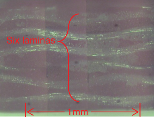

Figure 3 shows a composite specimen and also a patterned specimen surface prepared for DIC. High contrast speckle patterns were applied using a thin coat of white enamel paint and a diffuse overspray of black enamel so that the appropriately patterned specimen surface can be used effectively in 3D-DIC to obtain out-of-plane deformations and surface strains throughout the region of interest.

Figure 3.

Specimen with applied random pattern for three-dimensional digital image correlation.

Preliminary monotonic tensile tests to failure were performed to obtain basic material property data using an MTS 810 50kip hydraulic test frame with hydraulic platen grips. Stereo digital image correlation²⁷ was used to measure the surface strain during each experiment. For each fiber orientation, the results were averaged from three experiments. The final stress–strain curves are shown in Figure 4.

Figure 4.

The stress–strain curves for specimens cut in six directions.

Table 1 presents the as-measured elastic moduli for fiber orientations θ = 0°, 15°, 30°, 45°, 60° and 90°. The data in Figure 4 is consistent with previous work of Reifsnider and co-workers.^8–10

Table 1.

Longitudinal Young's Modulus, E_θ, determined by linear regression using σ_xx – ɛ_xx data for individual specimen orientations, θ.

θ (°)	0	15	30	45	60	90
E_θ(GPa)	25.9	23.5	16.8	14.6	16.5	23.2

To determine the orthotropic elastic engineering constants, only the linear parts of the stress–strain relationship are used. Details regarding the optimization procedures used to obtain the composite properties were recently reported in the literature.²⁸ The orthotropic composite elastic properties obtained using a non-linear least squares approach are shown in Table 2.

Table 2.

Primary elastic properties for orthotropic composite²⁸.

E₁ (GPa)	E₂ (GPa)	G₁₂(GPa)	ν₁₂	ν₂₁
26.2	23.2	5.1	0.15	0.13

Integrated stereovision and compression–bending loading systems

A schematic of the compression–bending specimen and the loading process is shown in Figure 5. All specimens were initially placed in a Tinius Olsen TI-5000 electro-mechanical load frame in a nominally straight configuration. Compressive load, P, axial displacement, Δ, and out-of-plane offset from axial centerline, δ, are the primary parameters for our studies.

Figure 5.

Schematic of compression bending specimen, with load, P, offset, δ, and axial displacement, Δ.

To perform combined bending–compression loading of specimens such as those shown in Figure 3 while simultaneously acquiring stereo images of both sides of the specimen, an integrated experimental setup was designed that includes the loading fixture (Figure 5), specimen (Figure 3) and two independent stereovision systems. Figure 6 shows the complete experimental system, including stereovision systems and loading grips. Details regarding important experimental considerations are given in the following sections.

Figure 6.

Integrated compression–bending loading frame with dual stereovision systems. 0 and 1: stereosystem viewing compression (tension) surface; 2 and 3: stereosystem viewing tension (compression) surface; 4 and 5: stiffened stereo-camera holding device; 6: Tinius Olsen 5000 loading frame; 7: light sources; 8: stiffened platens connecting TI-5000 to specimen grips; 9: precision load cell; 10: end grips with free out-of-plane rotation and arbitrary load offset.

Tinius Olsen 5000 loading frame

The Tinius Olsen 5000 (TI-5000) electromechanical test frame (item 6 in Figure 6) was modified for use in our studies. The grip speed of TI-5000 is 0.25–500 mm/min with different displacement resolution, depending on the required displacement resolution.

The accuracy of the displacement sensor is 0.0063 mm for grip speeds <12.5 mm/min, which is the range used in our experiments. The maximum force capacity is 22.25 kN with resolution 0.67 N. This accuracy is unacceptable for our experiments, where the maximum load is typically less than 35 N. To overcome this limitation, a high accuracy load cell (Honeywell Model 102, S-shaped design) was integrated into the loading frame. The load range is +/−196 N with 0.04 N resolution. The load cell is shown as an inset in the top left corner of Figure 6.

Specimen grips

Given the relatively small mechanical loading that will be applied to the specimens during either monotonic loading to failure or during cyclic loading to a pre-specified maximum axial displacement, an end grip was designed to provide well defined end conditions (see Figure 7). First, a needle roller bearing was integrated into the grip to allow free out-of-plane rotation of the specimen during bending to simplify analysis of the specimen and ensure the central location along the length corresponds to the maximum moment location (e.g. approximates the critical location) during both monotonic and cyclic loading. Second, the specimen was positioned in the grip using two small screws and various shim thickness to provide an offset that resulted in a small applied bending moment to minimize specimen buckling effects. Third, the grip was machined to include an inclined plane so that the large bending deflections incurred under monotonic loading would not be restricted by the grip shape; out-of-plane end rotations larger than 90° were obtained for some fiber orientations. Finally, the small gripping section of the fixture was manufactured from brass with minimum mass to reduce the moment of inertia and limit its effect during planned future higher frequency fatigue experiments.

Figure 7.

Specimen grip.

Control system

Results from preliminary compression–bending experiments confirmed that the compressive load reaches a relatively constant, low value (about 80% of maximum force) for Δ > 0.25 mm, resulting in instability when performing experiments in load control (which is preferred for use in future modeling studies). To deal with this issue, an external, software–hardware system was developed and interfaced with the TI-5000 for performing low load, large displacement bending–compression experiments. Specifically, the investigators developed the control system so that control can be readily shifted from displacement to load during the experiment, providing a stable platform for experimental studies while also ensuring that load control is possible in those regions (e.g. nominally elastic) where possible.

To perform the loading process in a manner that allows control of (a) axial displacement, Δ, of the specimen and/or (b) axial load, P, of the specimen and (c) acquisition of simultaneous images from all four cameras at a pre-specified combination of Δ and P, the entire TI5000 control system was analyzed, modified to meet our requirements and then controlled using a National Instruments (NI) LabView software (version 8.2) program. The program was written to automate the mechanical loading and data storage procedures. Figure 8 provides a flow chart for the automation process. In this study, NI device BNC adapter 2110 was used for analog input, analog output and trigger/counter functions. The NI data acquisition (DAQ) device PCI-6023E was used for high-performance multifunction analog, digital and timing I/O. The investigators manufactured custom-made serial cable (a 9 pin to 25 pin cable for output/input of data from various channels) and used the cable for all communication with the TI-5000.^b

Figure 8.

Flow chart for Labview program controlling all I/O functions for TI-5000.

Four-camera stereovision system

Since the combined compression–bending studies will result in large out-of-plane motion and substantial in-plane strains, a dual stereoimaging system with 3D-DIC is employed to accurately and simultaneously measure surface deformations on both surfaces during the loading process. Figure 6 shows the two complete stereovision systems in the configuration used for our studies. Table 3 summarizes the specifications for the system. Since the two stereovision systems are viewing separate surfaces of the specimen, there are several issues that require discussion including (a) lighting, (b) depth of field (DOF) and field of view (FOV), (c) mounting system and camera positioning (d) specimen patterning for large out-of-plane displacement, (e) calibration and (f) measurements.

Table 3.

Specifications for stereovision systems.

Camera types	Point grey (compression side)	Q-imaging (tensile side)
Pixel resolution	2448 × 2048	1360 × 1036
Lens focal length	55 mm	55 mm
Nominal optical F#	22	22
Object resolution (square pixels)	32.3 pixels/mm	18.2 pixels/mm
Distance to specimen	0.4 m	0.4 m
Synchronization^a	1 µs	1 µs

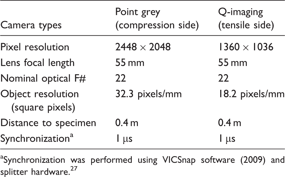
Synchronization was performed using VICSnap software (2009) and splitter hardware.²⁷

Lighting

First, lighting for each stereovision system is provided by at least two halogen lamps. As shown in Figure 6, the halogen lights are located at least 1 m from the specimen. To minimize heating of the specimens, a robust IR filter is used for each halogen light.^c Each set of cameras is mounted firmly to a cross-beam to minimize vibration throughout the experiment.

DOF and FOV

Since preliminary experiments indicated that out-of-plane displacements up to 40 mm will occur during the bending–compression experiment for the 45°/45° fiber orientation, the combination of (a) required DOF and (b) the relatively close camera positioning required to obtain high resolution images for strain field determination across the width of the specimen necessitated an analysis of both the DOF and FOV prior to performing experiments. Using the procedure outlined in the study of Sutton et al.²³ with the tabulated specifications in Table 3 and an assumed 10 µm spot size, DOF ≈ 24 mm. For an object distance of 0.40 m, focal length of 0.055 m and a CCD sensor size of 0.0127 m, the angle of view is ≈13.2° and FOV ≈ 90 mm × 90 mm. Based on this information and the geometry of the specimen, it is clear that (a) approximately one-half of the specimen length can be imaged by both stereovision systems and (b) there may be slight blurring of the specimen at maximum displacement in the central region, where displacements are largest during bending.

Camera positioning and orientation

To optimize the positions of the two stereovision systems, a modified version of the procedure outlined by Sutton et al.²⁹ is employed. In the bending–compression experiment, the compression side of the specimen moves away from cameras and the tension side moves towards the cameras. So the investigators performed a preliminary experiment where (a) the compression side camera system is placed as close to the undeformed specimen as possible while maintaining reasonable focus and (b) the tensile side camera system is placed as far from the undeformed specimen as possible while maintaining adequate focus. Results from a series of out-of-plane translation experiments ranging from 0 to 40 mm confirmed that the images on both sides of the specimen were sufficiently focused throughout the experiment and image correlation was performed successfully, with strain variability consistent with previous, well-focused experiments. As a result, this procedure was used to set up the stereovision systems for all experiments. The as-constructed imaging configuration deviated slightly from previous theoretical estimation, resulting in a FOV of 75 × 60 mm, which extends beyond the specimen mid-span and hence is adequate for our studies.

With regard to the specimen region being viewed, it is noted that the axial displacement, Δ, on one end of the specimen ranges up to 90 mm during monotonic compression–bending loading. To eliminate this issue, stereoimaging on both the compression and tension sides of the specimen was performed on the lower one-half of the specimen where the grip is stationary.

Finally, preliminary experiments confirmed that the compression–bending process resulted in out-of-plane specimen rotations that approached 90° at the stationary end. To ensure that image correlation could be performed along most of the specimen length, both stereovision systems were initially configured as shown in Figure 9. By orienting and positioning the systems as shown, the deleterious effects of subset foreshortening due to rotation were minimized and image correlation could be performed successfully for the entire FOV on the specimen.

Figure 9.

Schematic of positioning and orientation of stereovision systems for compression–bending composite specimen experiments. Compression (tension) side vision system rotated counterclockwise by ≈20°, moved closer (further) from specimen and translated vertically upward (downward) by ≈20 mm.

Speckle patterning

Regarding speckle patterning, as noted in a recent publication,²³ oversampling requires that each speckle be sampled by at least 3 × 3 pixels for optimal accuracy. Thus, the minimum speckle sizes would be ≈0.2 mm on the tension side and ≈0.11 mm on the compression side. However, due to the presence of large out-of-plane displacements, images of the speckles will decrease (increase) substantially on the compression (tension) sides. In our studies, a slightly larger speckle size was used to ensure oversampling of each speckle throughout the experiment. To apply the speckle pattern, an airbrush with 0.5 mm needle is used to spray a relatively homogeneous spot pattern spot. By moving the specimen closer (further) from the nozzle, a larger (smaller) pattern is generated on the compression (tension) surfaces of the specimen. Here, the as-produced average speckle sizes are 0.4 mm (0.3 mm) on the compression (tension) surfaces. Figure 3 shows a typical speckle pattern produced on the compression side of the specimen.

Calibration

Stereovision calibration was performed simultaneously for both systems using the procedures described in previous publications^23,29 (see chapter 7.2 in Sutton et al.). Briefly, a specially designed planar target is manufactured with through-thickness circular white cylindrical markers embedded in an orthogonal array within a nominally black plate having a constant thickness, t +/−10 µm. After positioning both systems as shown in Figure 9, images of the translated and rotated target are acquired simultaneously by both stereovision systems. Each system is then calibrated using images from separate sides of the target. Finally, the calibrated imaging systems are then converted to a common orthogonal coordinate system by relating ‘specimen coordinate systems' defined for each stereovision system and the known target thickness. The common orthogonal coordinate system used for all measurements is shown in Figure 10.

Figure 10.

Side view and perspective view of composite specimen with common Cartesian coordinate system. The X coordinate is along specimen length; Y coordinate is measured from specimen centerline in the width direction. The Z coordinate is in the thickness direction.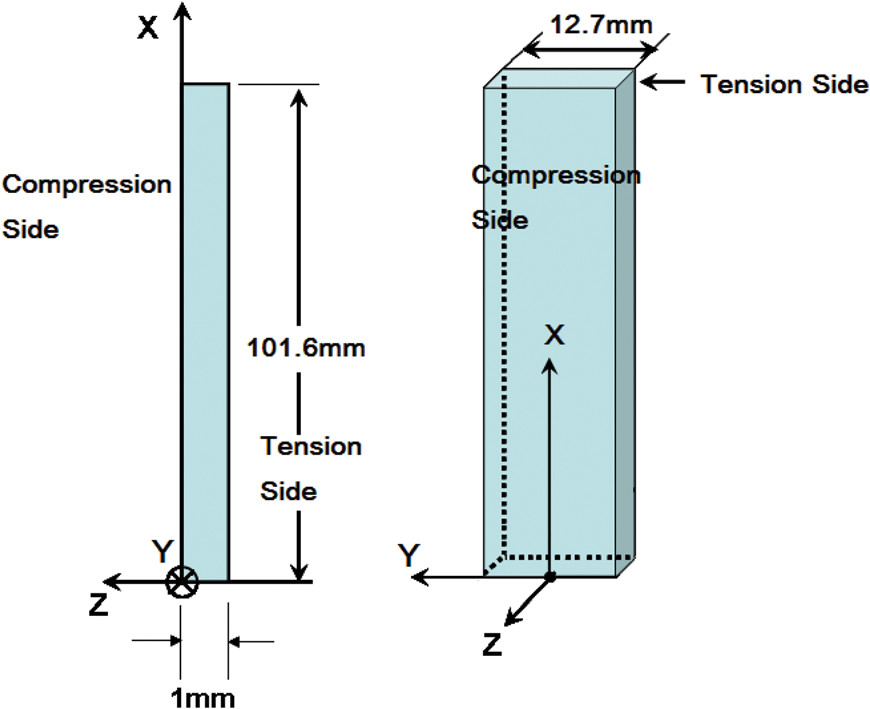

Measurements

During the experiments, stereoimaging was used to obtain the following full-field data at selected loads and axial displacements (a) 3D object displacement components (u, v and w) in the X, Y and Z directions, respectively and (b) in-plane strain data (ɛ_xx, ɛ_yy and ɛ_xy). Unless otherwise noted, a 31 × 31 pixel subset size with a subset spacing of 10 pixels is used in all analyses. According to object resolution in Table 3, the physical subset size is about 1 mm and 1.5 mm corresponding to the compression side and tension side, respectively, which is similar to the weave length (see Figure 1). Strain data was extracted from the displacement measurements using procedures described previously.^23,27,29 Briefly, all displacement components (u, v and w) are converted to a global coordinates system located at the original position in the reference configuration (see Figure 10) to obtain 3D displacement fields. Partial derivatives of the displacement field are computed from a quadratic polynomial least square fit to the computed displacement field in a local neighborhood; in this study, a 5 × 5 set of displacement data is used to determine the quadratic best fit for each displacement component. The Lagrangian strain tensor is defined at the center of the polynomial fit in terms of the gradients of the displacement vector components.²³ The preliminary results show that, after calibration, the range of strain values is less than ±200 microstrain.

Experimental results and discussion

A series of monotonic bending–compression experiments were performed on composite specimens with various fiber orientations. All experiments were performed with sinusoidal actuation controlled automatically by the Labview program, which keeps the overall average speed constant at 0.21 mm/s (0.5in./min); the maximum displacement rate does not exceed 0.33 mm/s.

Axial load and centerline moment versus axial displacement

Figure 11 presents the measured axial load, P, versus measured axial displacement, Δ, up to final failure for all fiber angles.^d As shown in the expanded view of the early stages, in the range 0.05 mm ≤ Δ ≤ 0.10 mm, the load reaches a constant value that is a function of fiber angle for axial displacements. For low fiber angles relative to the loading direction, the orthogonal weave specimen has a rising load–displacement behavior up to maximum load. For fiber angles ≥30°, the initial linear region transitions to a falling load regime that eventually leads to a rising load prior to final failure. It is noted that ordering of the initial load plateau magnitudes for 0° (90°) fiber orientation are consistent with predictions using Euler buckling load formulation and the elastic modulus E1 (E2) in Table 2.

Figure 11.

Typical load versus end displacement.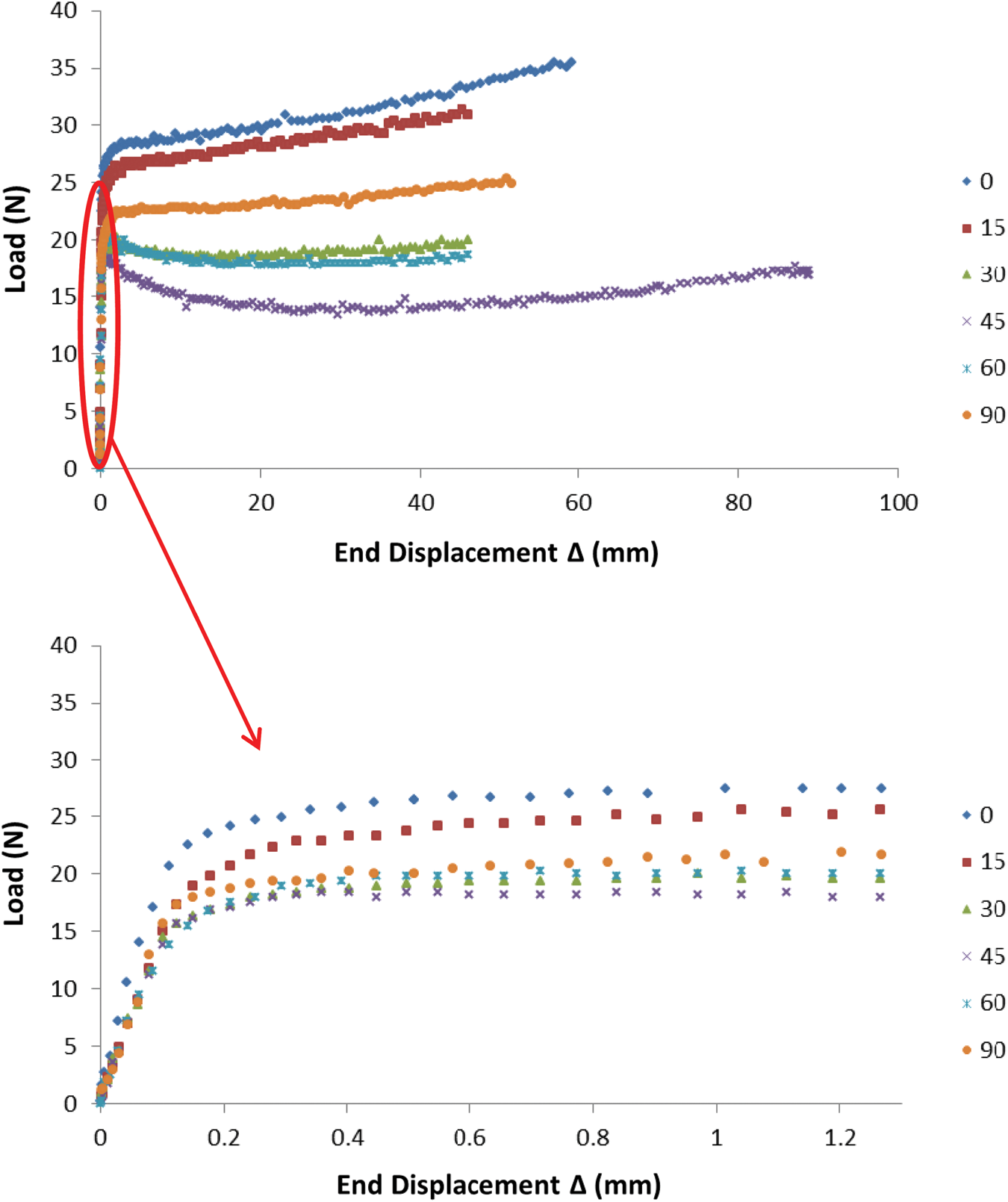

Using the measured out-of-plane displacement field, w(x, y, z), which is obtained in a full-field manner by our stereovision systems using 3D-DIC at various load levels, the maximum moment in the specimen was determined using the formula M_max(x = 50.8 mm, y = 0, z = 0.50 mm) = P • (δ + ½ (w(50.8 mm, 0, 0) + w(50.8 mm, 0, 1 mm). Figure 12 shows the maximum bending moment at mid-length versus the axial compressive displacement, Δ. As shown in Figure 12, even for large deformation conditions where the applied axial loading is relatively constant, the measured bending moment is a monotonic function of end-point displacement throughout the loading process for all fiber angles. Furthermore, even though the axial loading is relatively constant for various angles, the maximum moment results are ordered in the same manner as both the elastic moduli of the specimens (see Table 1) and the P−Δ data shown in Figure 11.

Figure 12.

Typical local M_max versus Δ data at mid-length of specimen.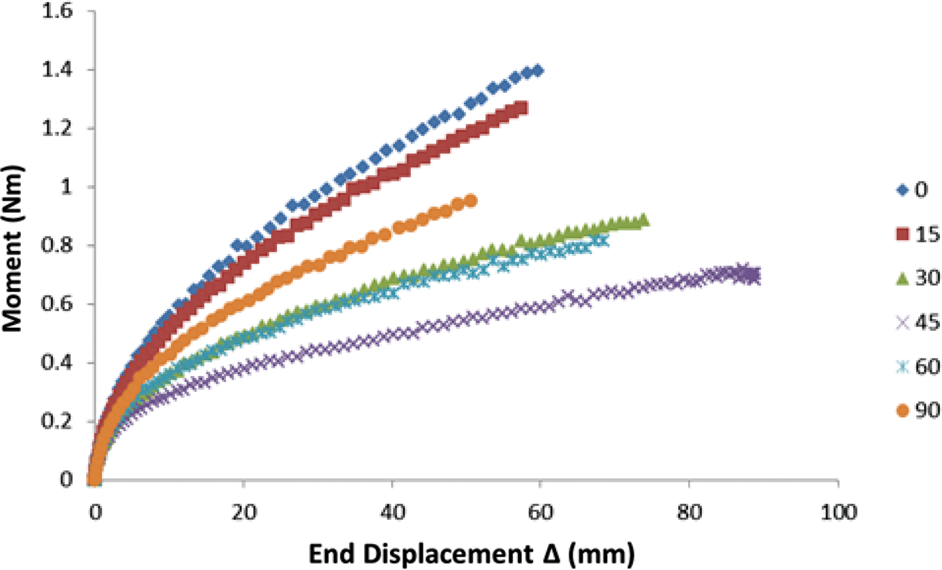

Surface strain measurements

In addition to the global parameter results shown in Figures 11 and 12, stereovision with 3D-DIC provides full-field measurement capability for the surface strains along the length and width of the specimen within the FOV. For the same axial displacement (Δ = 40 mm), Figure 13 shows typical axial strain fields, ɛ_xx, on both the tension and compression surfaces of the specimen for (a) θ = 0° and (b) θ = 45°; the black mark on each surface denotes the approximate mid-length location.

Figure 13.

Measured axial strain field, ɛ_xx, on tension and compression sides for both θ = 0° and θ = 45°.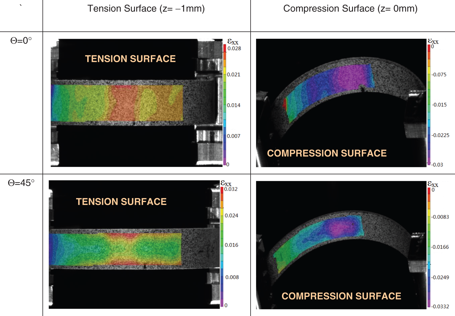

Strain Localization, θ = 0° and 45°

As shown in Figure 13, for θ = 0° strain localization occurs across the entire specimen width for both the tension and compression surfaces near the mid-length (maximum moment) location. At this location, ɛ_xx^max≈ + 0.025 on the tensile surface and ɛ_xx^min≈ −0.03 on the compression surface. In addition, curvature measurements along the length clearly show distinctly higher curvature (lower radius of curvature) in the central region where strain localization is most evident.

The difference in maximum strains between the tensile and compressive surfaces is physically relevant and requires additional discussion. For θ = 0°, the fibers are oriented along the maximum (minimum) strain direction. As indicated in Figure 14 for lower fiber angles (θ = 0° and θ = 30°), macroscopic visual evidence clearly shows the presence of local fiber buckling on the compression side; broken fibers protruding from the specimen surface and complete loss of speckle pattern are clearly visible as the loading proceeds and the curvature increases locally. In fact, micro-buckling can be observed by the naked eye on the compressive side of the specimen for all θ ≠ 45°. The onset of visible micro-buckles is a pre-cursor to final failure of each specimen, indicating that the ultimate collapse is primarily due to local geometric instability and local fiber buckling on the compression surface of the specimen. Conversely, on the tensile side there was no clear evidence of fiber failure, though there was some evidence of matrix micro-cracking.

Figure 14.

Macroscopic photo of compressive surfaces and effect of micro-buckling for θ = 30°(top) and θ = 0° fiber orientations.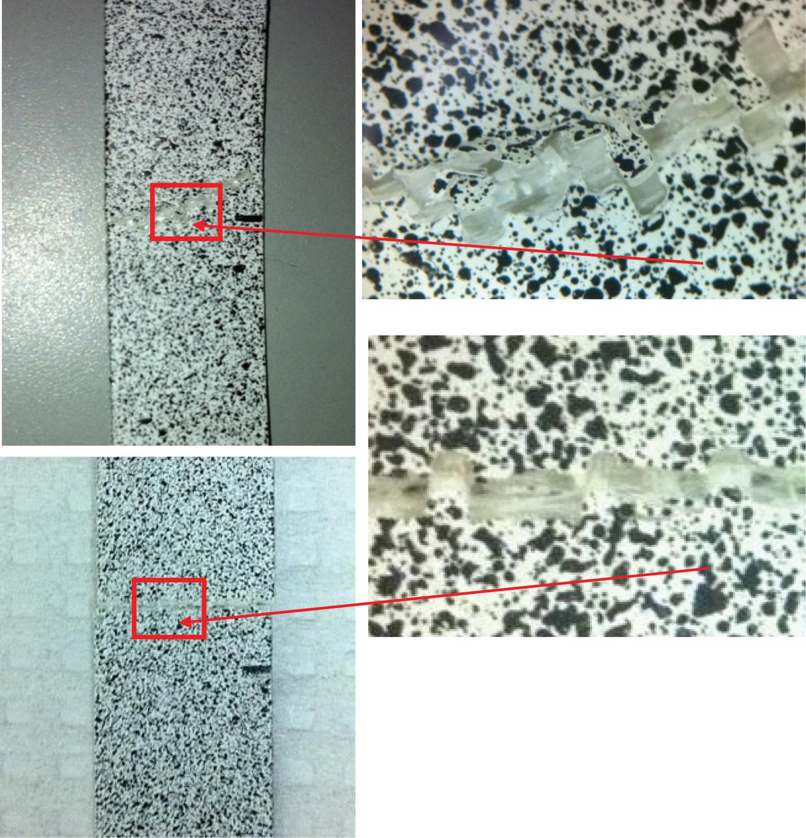

Thus, the localized region of higher compressive strains is a direct consequence of local damage mechanisms that are well known to be distinctly different between the tensile and compressive regions in the specimen.

For θ = 45°, again there are distinctly different strain localization fields on the tension and compression surfaces. On the tensile surface, an hour-glass shaped region is observed where the maximum axial strains occur at the specimen edges. The region is bounded by lines at +/−45°, which correspond to the fiber angles of the orthogonal weave. Thus, the higher axial strains near the unrestrained specimen edges are consistent with matrix deformation in low constraint regions due to the effect of the free edges. Conversely, lower strains in the central portion of the hour-glass region are consistent with increased constraint on the fiber structure imposed by the surrounding orthogonal fiber weave. On the compression side of the specimen, the highly localized strain field shows the reverse trend; significantly higher strains in the central region and lower strains on the edges of the specimen. The increased strains in the central region are consistent with matrix-dominated response for this higher fiber-angle specimen. The lower compressive strains near the specimen edges again appear to be related to ‘free-edge’ effects.

Figure 15 shows a typical spatial relationship between the beam centerline and the position of the final failure point (which usually has maximum axial strains on both the tension and compression surfaces). Results from our studies indicate that the final failure region occurs within one-half of the specimen width from the specimen centerline and most often slightly towards the stationary end in Figure 9. Since random variations in the fiber distribution/weave during manufacture are inconsistent with this observation, slight asymmetry in the mechanical loading system components (e.g. grips, alignment) is considered to be the most likely source of the preferential shift in failure position.

Figure 15.

Relationship of critical area and geometry center of specimen.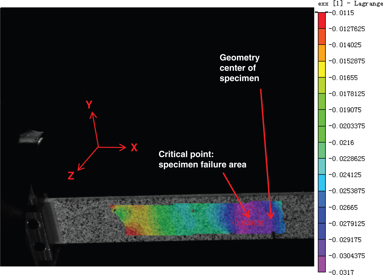

As one would expect, the evolution of maximum axial strain in the critical region is a function of fiber angle and whether the compression or tensile specimen surface is considered. Figure 16 (compared with Figure 17) shows the evolution of ɛ_xx axial strain^e on the compression (tension) surface of the specimen. Appendix A shows the evolution of both the transverse strain ɛ_yy and the shear strain ɛ_xy on the compression (tension) surface as a function of fiber angle in the same critical region.

Figure 16.

Average ɛ_xx strain in critical region on compression surface of specimen versus bending moment.

Figure 17.

Average ɛ_xx strain in critical region on tensile surface of specimen versus bending moment.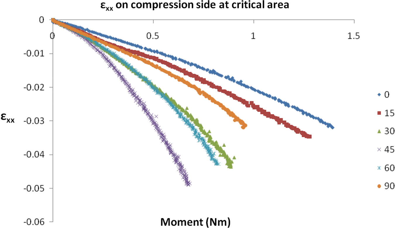

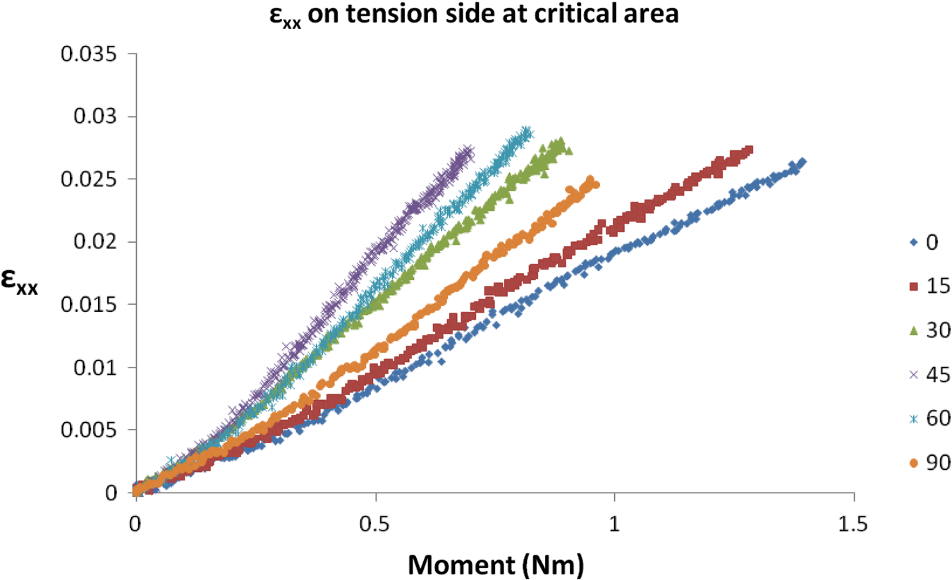
Comparison of Figures 16 and 17 indicates that the measured axial strains on the compression side for all fiber angles are much higher than on the tension side. Such an observation is nominally consistent with the observed presence of micro-buckling in the critical region for θ ≠ 45° and suggests that the effective bending neutral surface of the damaged specimen has shifted towards the tension surface. Further evidence of a shift in the bending neutral surface is the nature of the bi-linear (changing slope) functional form for the tensile strain data; a shift in slope of the strain–moment data occurs when ɛ_xx ≥ 0.005, suggesting that compression-side damage via micro-buckling occurred prior to these strain levels. The observation that the tensile strain field remains linear until reaching maximum axial displacement indicates the damaged fiber–matrix structure on the tension side has relatively constant resistance to the increasing moment. Conversely, the continuing non-linear strain–moment relationship on the compression surface for all fiber angles is consistent with increasing damage and decreasing resistance to the moment in this region up to specimen collapse.

Anticlastic curvature

For Δ < 5 mm, our w(x,y) measurements indicate that nearly the same primary and anticlastic beam curvature are present along the specimen length for all fiber orientation angles; if w(x,y) data for each fiber angle and a specific Δ < 5 mm were plotted together, the results are nearly the same. However, for larger Δ, the investigators observed the presence of double curvature near the critical region of the compression–bending specimen, especially for increasing primary curvature (large Δ implies large w(x,y) and hence larger curvature), for all fiber angles.

The largest anticlastic curvature (warping) occurred near mid-length in the 45°/45° specimen for relatively large Δ. Figure 18 shows typical double curvature measurements in a 45°/45° specimen with Δ ≈ 40 mm. At the top left of Figure 18 is the 3D shape of the left-half^f of the 45°/45° specimen. At the bottom left is the out-of-plane displacement data for the center line of specimen. Figure 18 indicates that the axial shape of the specimen in the bending–compression experiment approximates a sine curve when the deformation is not too large, which is consistent with the expected shape using Euler–Bernoulli beam theory with the small deformation assumption 1/ρ ≈ d²w/dx². This observation is due to the coupling that exists between the shape of specimen and the bending moment, which is proportional to the second derivative of deflection using small deformation theory. Further analysis in a forthcoming article shows that, for small deformations, this is quite accurate. For large deformations, the shape of specimen is more arched than a sine curve and a detailed equation description will be given using large deformation theory to show the origin of the differences in the forthcoming article.

Figure 18.

Full-field deflection data of 45–45 specimen.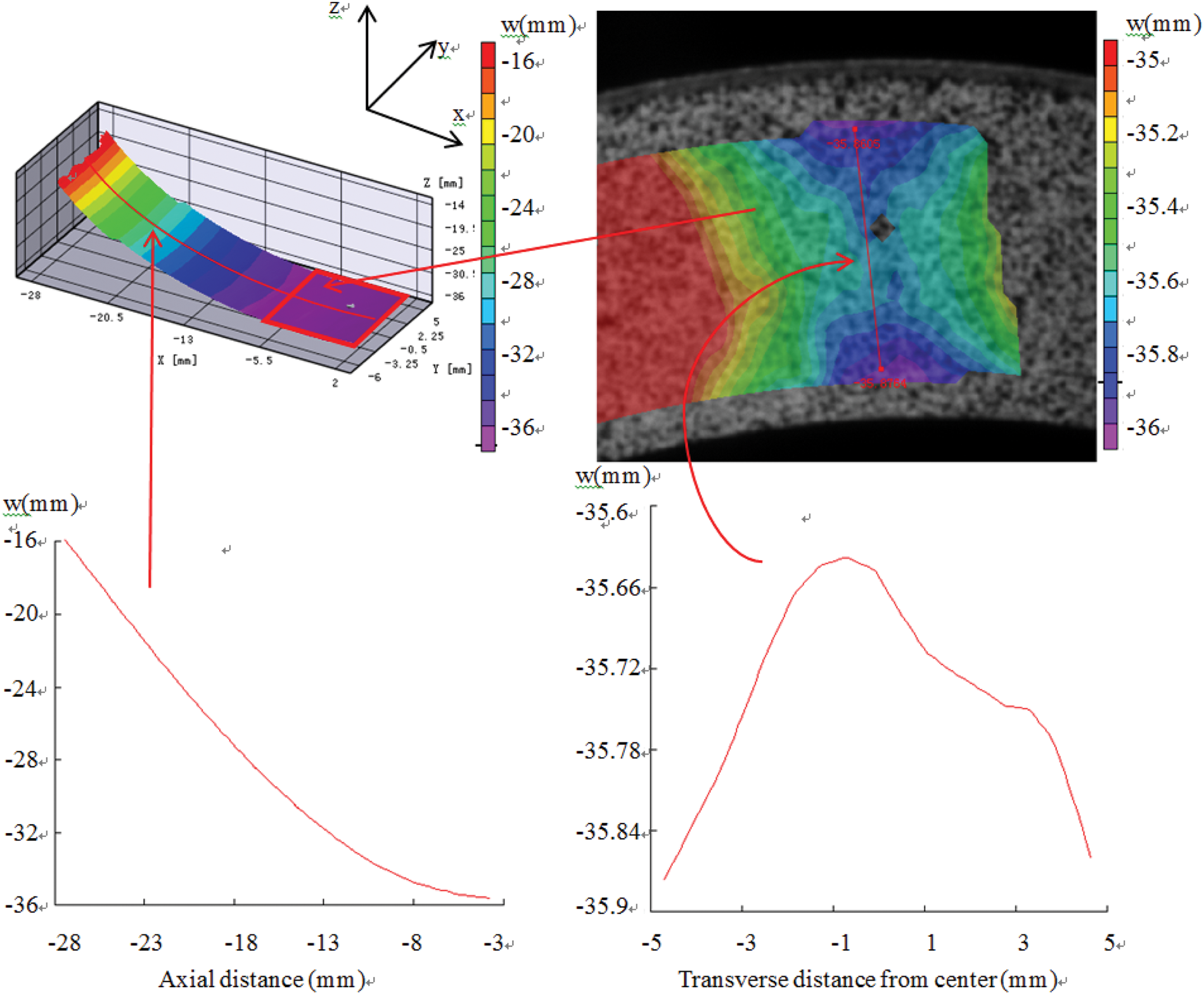

Also shown in Figure 18 is the cross-width shape of the beam on the compression surface in the critical region near the beam centerline. In this case, the difference in out-of-plane deflection between the center and edge of the beam, Δw ≈ 0.3 mm, is 30% of the thickness (h = 1 mm).

Figure 19 shows the normalized deflection ratio Δw/h for 0–90, 15–75, 30–60 and 45–45 specimens in the critical region near the specimen centerline for Δ ≈ 40 mm. Inspection of Figure 19 shows that Δw/h < 0.10 for 0–90 and 15–75 specimens. However, for 30°/60° and 45°/45° specimens, Δw/h exceeds 0.25 when Δ = 50 mm. For 30° ≤ θ ≤ 60°, the effect of anticlastic curvature appears to be significant in the critical region for values of Δ near final collapse. However, for lower fiber angles, Δw/h < 0.10 which suggests that, if a simpler analysis methodology is required, the effect is small and the deformations obtained by considering the response of an orthotropic material with two different Young's moduli may be sufficient.

Figure 19.

Normalized deflection difference along transverse direction.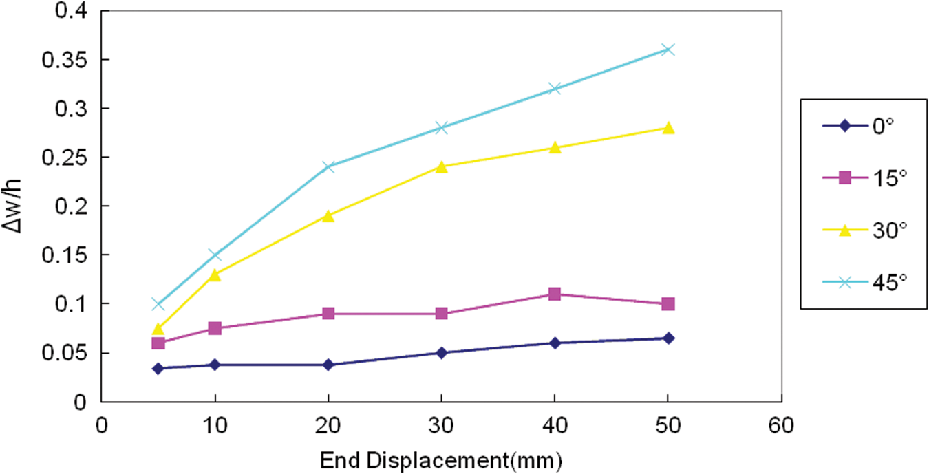

Though classical lamination theory (CLT) is not strictly applicable for our woven composite system, the authors have used CLT as a predictor for our specimen behavior in the small displacement regime. According to the mechanical properties given in Table 2, we can determine the extension–bending coupling matrix B to help understand the relationship between bending and in-plane strains.

For 0°/90° specimen, only B11 and B22 are non-zero terms in matrix B, which couple in-plane normal forces to bending curvatures, and bending moments to in-plane strains. Experimental evidence to corroborate the presence of coupling is shown in Figures 20 and 21. Here, it is clearly shown that the in-plane strain ɛ_xx increases with end displacement, which shows positive correlation with bending moment in Figure 12. Figures 16 and 17 gives this relationship more directly.

Figure 20.

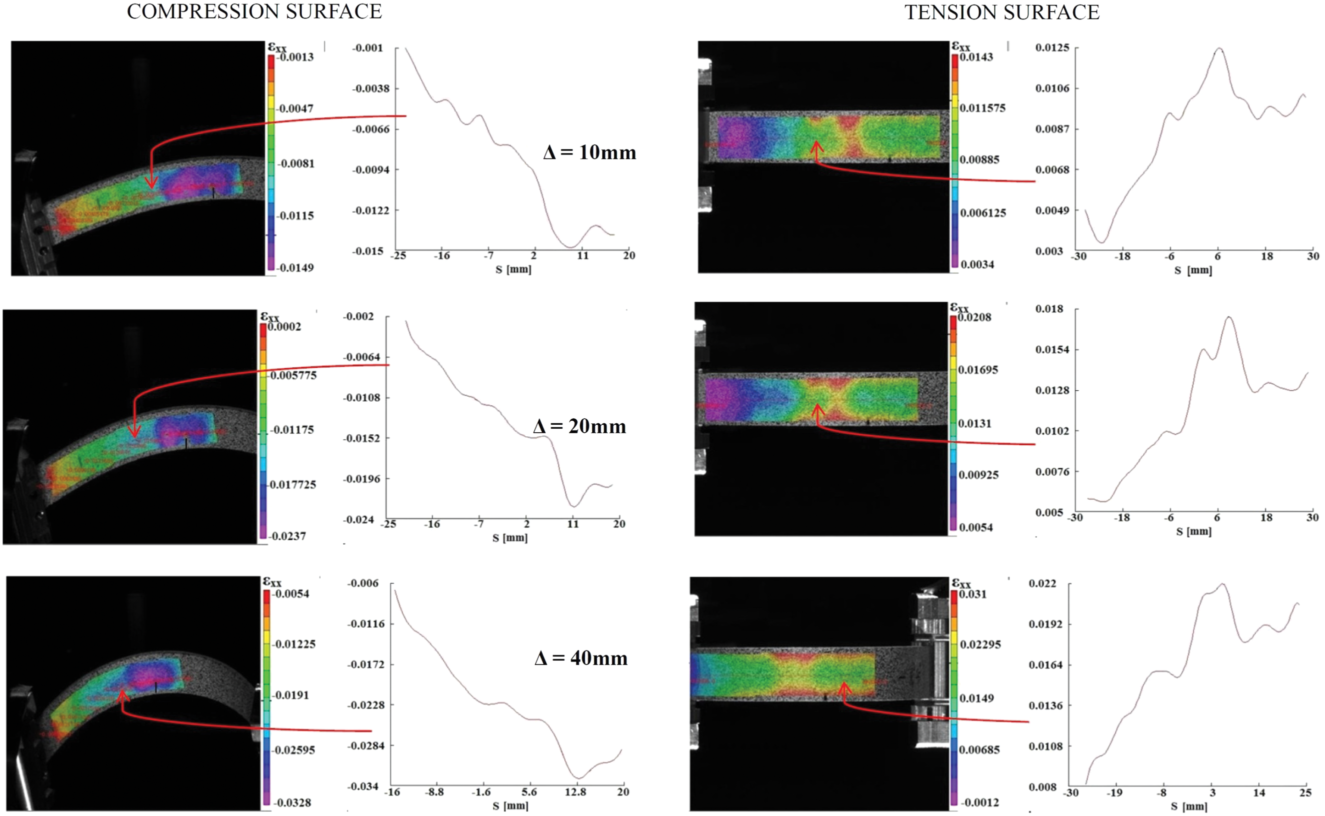
Axial ɛ_xx field and centerline plot of ɛ_xx on compression and tension surfaces of θ = 0°/90° specimens for Δ = 10, 20 and 40 mm.

Figure 21.

Axial ɛ_xx field and centerline plot of ɛ_xx on compression and tension surfaces of θ = 45°/45° specimens for Δ = 10, 20 and 40 mm.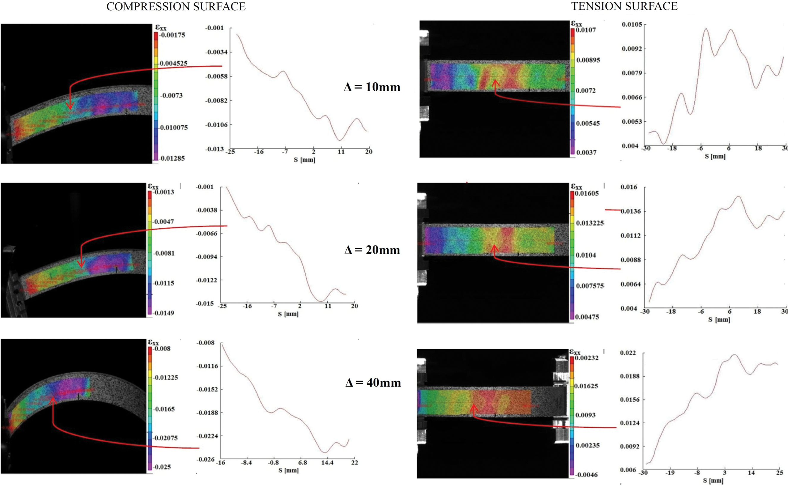

In addition, the authors used CLT to help explain the 0/90° specimen response after fiber buckling occurs on the compression side and stiffness is lost (less than 10%) along the axial direction. As the absolute values of B11 and B22 decrease, this leads to increasing in-plane compressive strain relative to the tension surface. This trend is shown in Figure 20 for the 0/90° specimen, where the compressive strain is considerably larger than the tensile values, resulting in through-thickness asymmetry in the axial strain distribution.

Also, CLT theory suggests there is no coupling between bending and in-plane strains for +/−45° fiber orientation. This prediction is consistent with observations documented in Figure 21, where even for very large axial displacements, the range in strain for ɛ_xx is nearly the same on both compression and tension surfaces.

Additional figures demonstrating the observed relationship between in-plane strain and end displacement are given in Appendix A.

Strain variations for small and large compressive displacement

Figures 20 and 21 shows the axial strain field ɛ_xx on the compression side and tension side of 0°/90° and 45°/45° specimens, respectively, when the end displacement Δ equals to 10, 20 and 40 mm. In each figure, both full-field data and a line plot in terms of arc length, S, of the data along the specimen centerline are shown. The S coordinate has the same direction as X coordinate, with origin identified by a red arrow on the left edge of the specimen. Appendix A presents the transverse strain field, ɛ_yy, and shear strain field, ɛ_xy, on the compression side and tension sides for 0°/90° and 45°/45° specimens, respectively, when the end displacement Δ equals 10 and 20 mm.

Axial Strain Field

Inspection of the tension surface data on the 0/90 specimen in Figure 20 clearly shows an oscillatory strain field for Δ = 10 mm that is considerably larger than the estimated variability in strain for our measurements. The oscillations in strain are somewhat muted as the deformation increases. These observations are consistent with the expected shear transfer process between fibers and matrix that requires sufficient distance to complete; the distance between peaks is ∼10 mm for our woven fiber–matrix material system, which is about 10 times of weave size of specimen and physical subset size of DIC and hence is resolvable by the stereovision measurement method. Conversely, for the 45°/45° specimen, all local peaks in axial strain are muted, suggesting that load transfer processes are relatively insensitive to axial position along the specimen for high fiber angle configurations.

As noted previously, for all fiber angles, the general shape of the beam-compression specimen is quite similar. Even so, the measured strains in the region of final collapse can be quite different, as well as the local curvatures. For Δ = 40 mm, Figure 22 shows the axial strain ɛ_xx distribution along the transverse direction on the compression side for the 0°/90° and 45°/45° specimens. It is clear that the strain differences along transverse direction are quite different, most likely due to the effect of increased anticlastic curvature for the 45°/45° specimen.

Figure 22.

Axial strain ɛ_xx distribution along transverse direction on compression side of 0°/90° (top) and 45°/45° (bottom) specimen, Δ = 40 mm.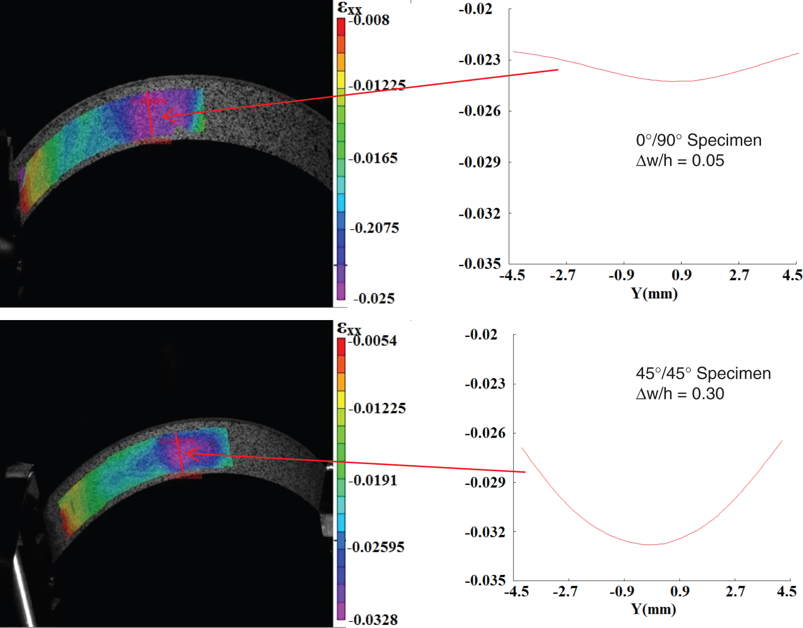

Fiber direction strains and axial–transverse direction strains in critical region

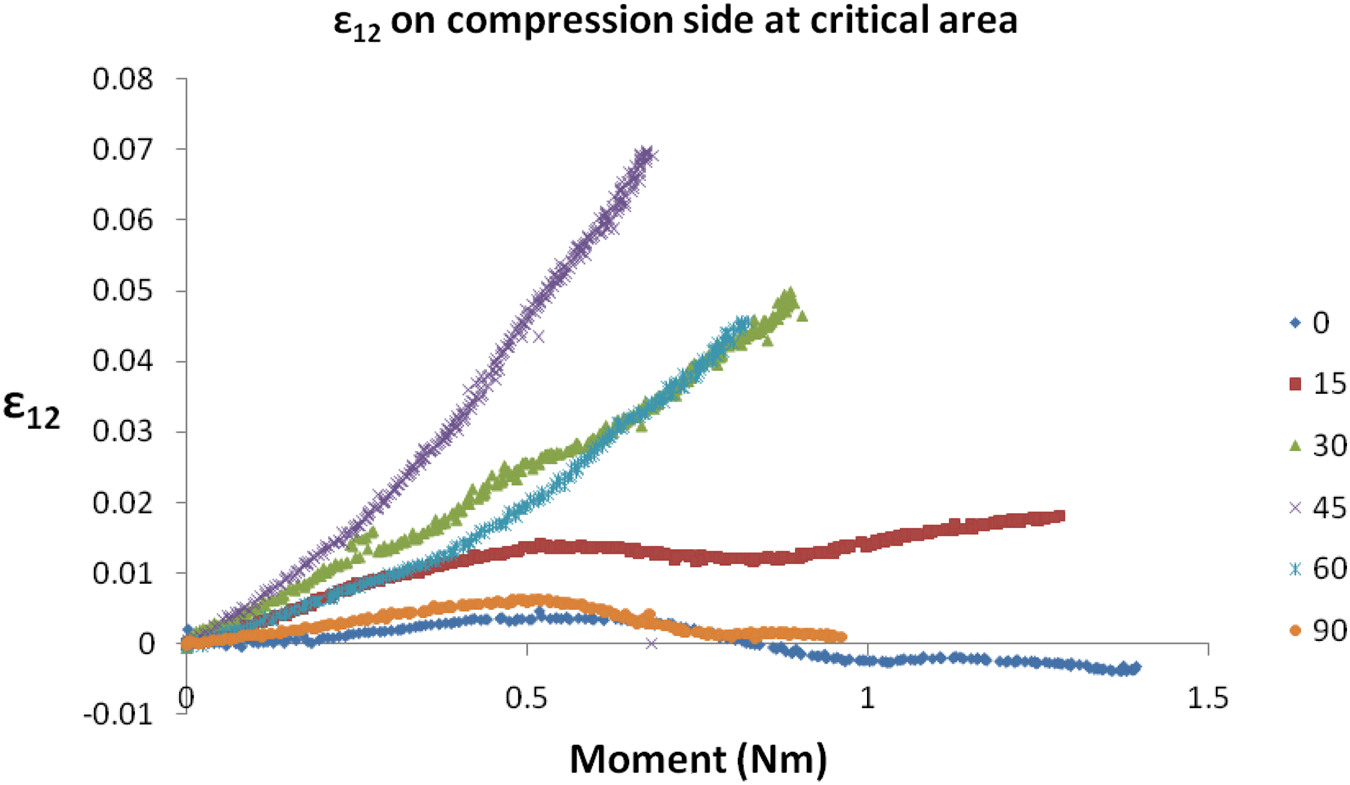
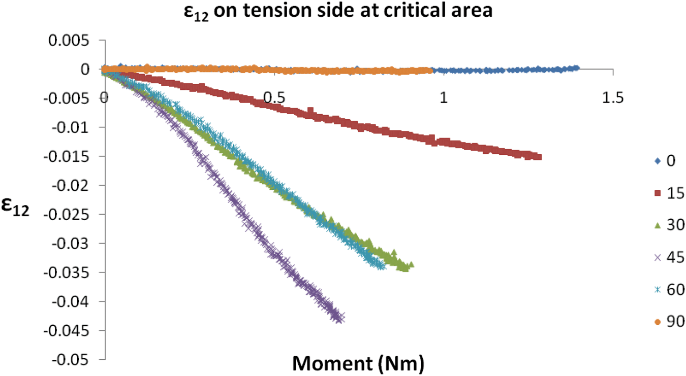
Using full-field data such as shown in Appendix A, the average ɛ_yy and ɛ_xy on both the tension and compression surfaces in the critical region were obtained^e as a function of applied moment. By transforming the measured strains from specimen coordinates (x,y) into the primary fiber directions (1,2), as shown in Figure 23, Figures 24 and 25 present the average fiber 2 strain, ɛ₂₂, versus moment in the critical region on both compression and tension surfaces for all fiber angles. Figures 26 and 27 present the average shear strain, ɛ₁₂, versus moment in the critical area on both the compression and tension surfaces for all fiber angles.

Figure 23.

Coordinate systems for transformation between specimen and fiber.

Figure 24.

Average ɛ₂₂ strain of critical area on compression surface of specimen versus bending moment.

Figure 25.

Average ɛ₂₂ strain of critical area on tension surface of specimen versus bending moment.

Figure 26.

Average ɛ₁₂ strain of critical area on compression surface of specimen versus bending moment.

Figure 27.

Average ɛ₁₂ strain of critical area on tension surface of specimen versus bending moment.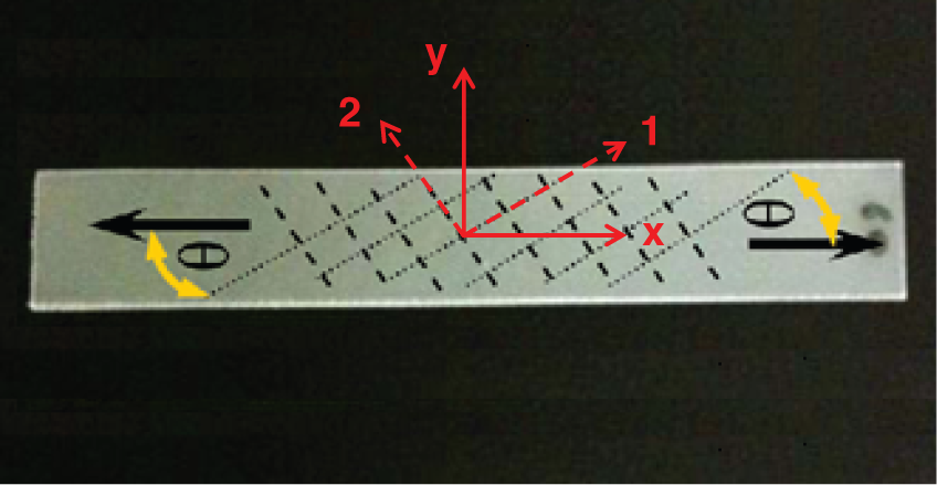

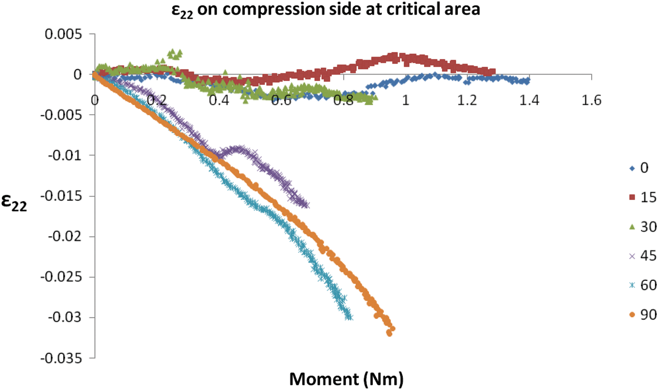
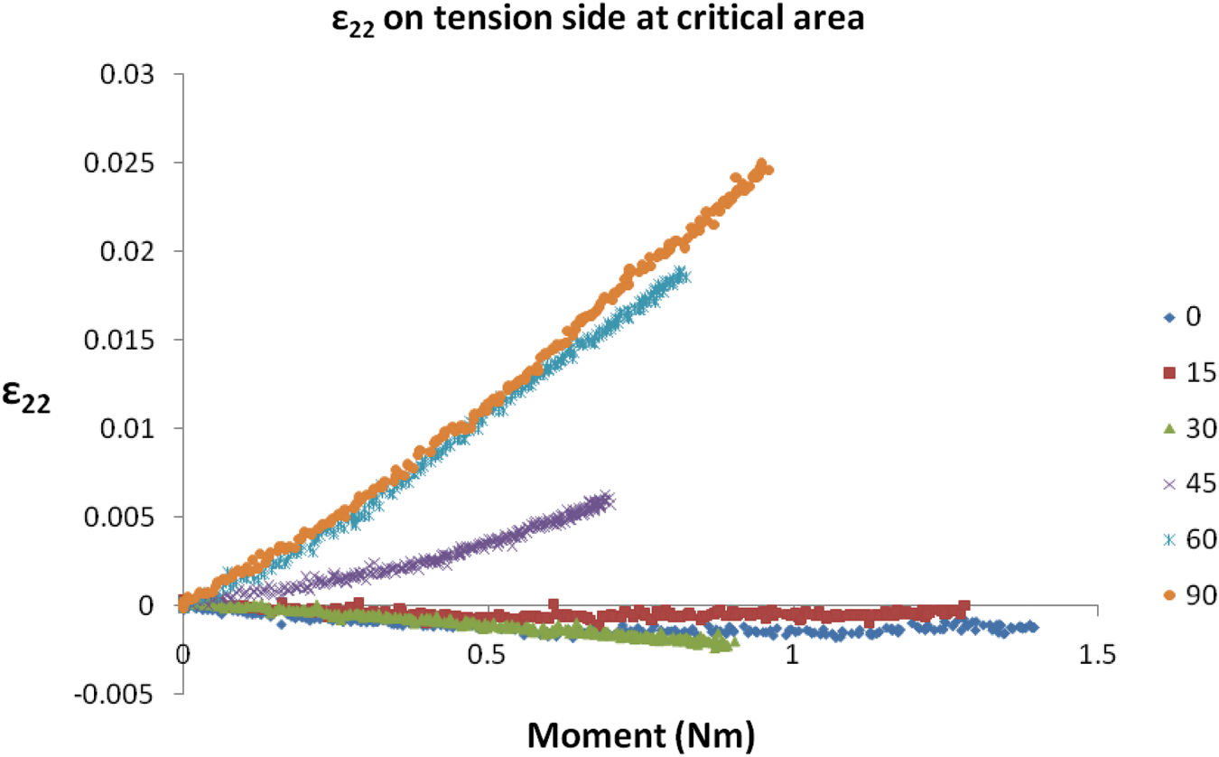
With regard to the strain ɛ₂₂, as shown in Figures 24 and 25 for 0°/90°, 15°/75° and 90°/0° specimens, ɛ₂₂ is small on both compression and tension surfaces, increasing for 45°/45°, 60°/30° and 90°/0° as fiber 2 direction orients more closely with the loading direction.

As shown in Figures 26 and 27, the shear strain ɛ₁₂ is negligible between the fiber directions for both 0° and 90° specimens, consistent with expectations and demonstrating that any fiber motions were essentially rigid rotations on the macroscale. With regard to other fiber orientations, as shown in Figure 26 (compare Figure 27), increasing positive (negative) shear strain was measured as the fiber angle increased from 15° to 45° or decreased from 90° to 45° on the tension (compression) surfaces. Thus, our measurements indicate that the fiber directions 1 and 2 rotated towards (away from) each other on the tension (compression) surfaces, an observation that is consistent with theoretical predictions and physical expectations.

Poisson's ratio

In addition to the fiber-oriented strain data, measurements reveal an approximate linear relationship between transverse strain ɛ_yy and moment for all fiber angles, consistent with the results in Figures 16 and 17, which show a linear relationship between axial strain and M_max. The results indicate that the ratio between axial and transverse strain is essentially constant throughout the deformation process. This is also true for 30°/60°, 45°/45° and 60°/30° specimens, which have much larger transverse strains (nearly 50% of axial strain).

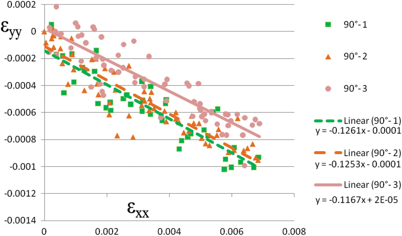
Using the measured axial and transverse strains for three 0°/90° and three 90°/0° specimens in small deformation region (maximum strain less than 0.8%), the investigators computed the average ν₁₂ and ν₂₁, respectively, for the specimen on the tension and compression surfaces. On the tension surface, the investigators obtained ν₁₂ = 0.152 +/−0.005 and ν₂₁ = 0.122 +/−0.005, which is graphically shown in Figures 28 and 29. This result is in good agreement with recent findings of Pollock et al.²⁸ where ν₁₂ = 0.15 and ν₂₁ = 0.13.

Figure 28.

ɛ_yy versus ɛ_xx on tension side for 0° specimens.

Figure 29.

ɛ_yy versus ɛ_xx on tension side for 90° specimens.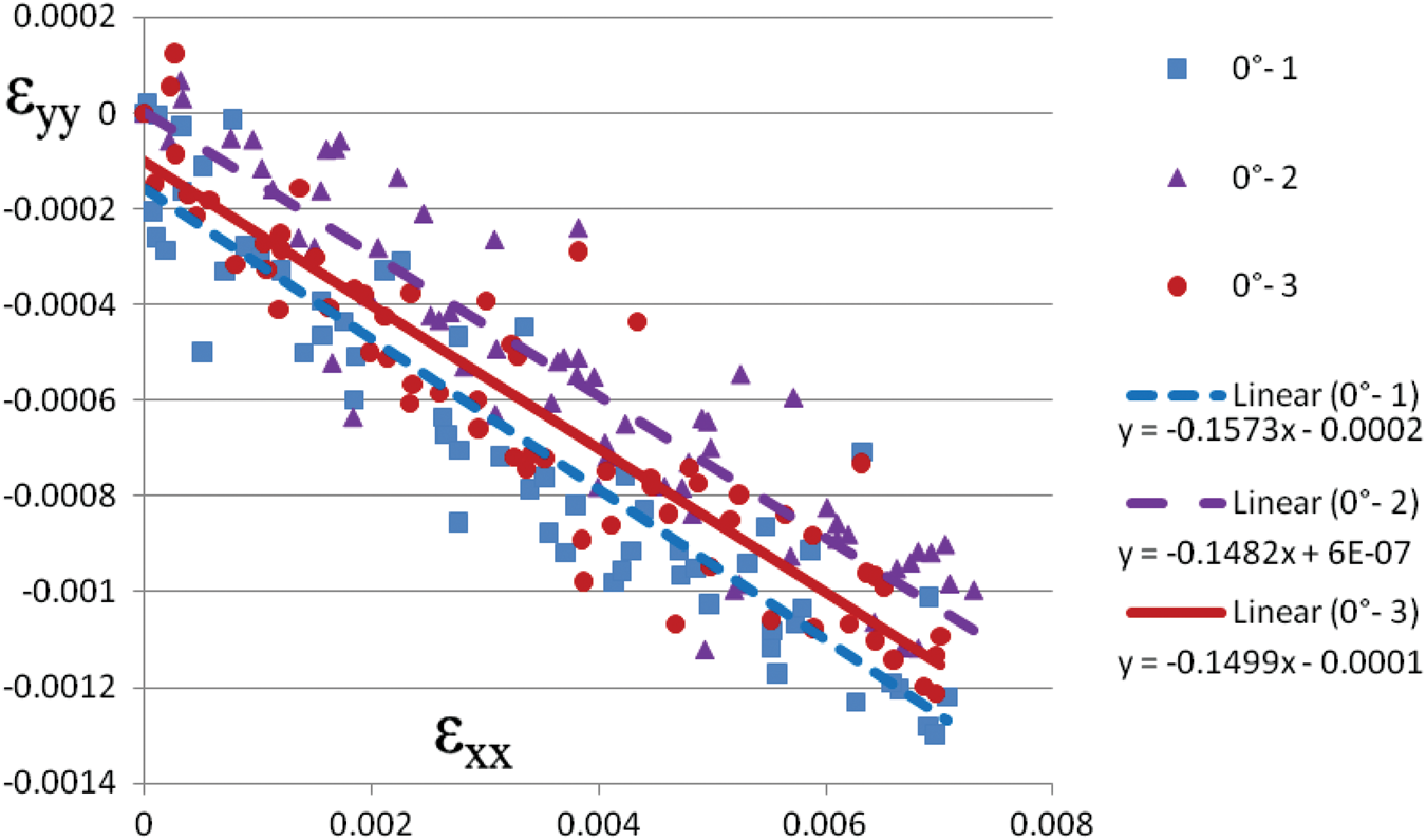

On the compression surface, the investigators observed a different behavior in Poisson's ratio. Graphically, this is shown in Figure 30 for 0°/90° and 90°/0° specimens. Though there is considerable scatter in the data in Figure 30, the investigators obtained ν₁₂ ≈ 0 and −0.10 ≤ ν₂₁ ≤ −0.40. With regard to the somewhat anomalous behavior on the compression side for Poisson's ratio, the investigators observed that Poisson's ratio on the compressive surface varied considerably across the specimen width at various axial positions. This anomalous behavior is also shown graphically in the ɛ_yy results on compression side presented in Figures A-1 and A-2. Specifically, our compression-surface measurements indicate that Poisson's ratio is small near the specimen centerline, becoming either negative near the edges or positive near the edges of the 0°/90° and 90°/0° specimens, depending upon the axial position that is selected. The variability shown in Figures A-1 and A-2 demonstrate that compressive effects in woven composite components can lead to highly localized deformations due to effects such as fiber buckling or crimping.

Figure 30.

ɛ_yy versus ɛ_xx on compression side for 0° and 90° specimens.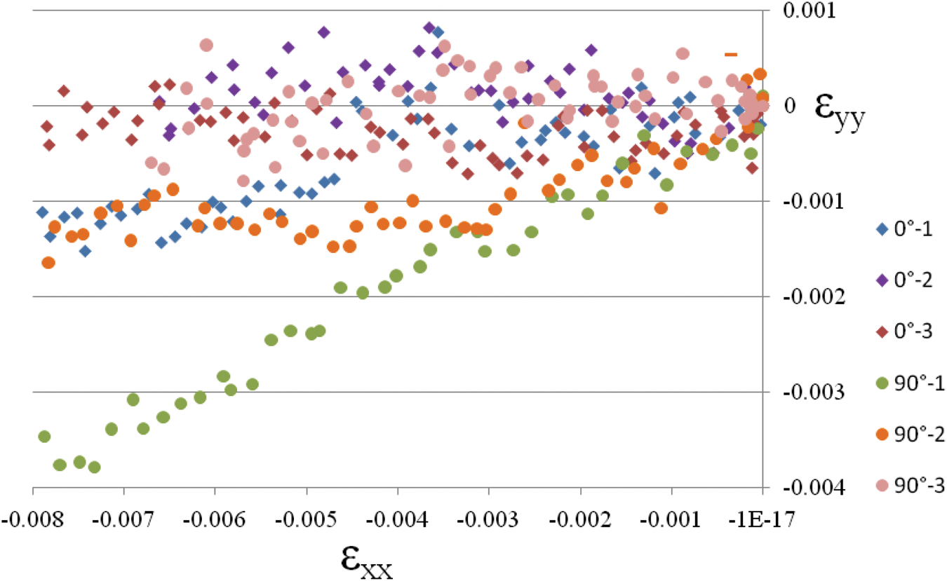

Figure 31 shows the experimental ɛ_yy/ɛ_xx results on tension side for all fiber orientation specimen and Poisson's ratio values quantitatively determined using the equations in the study of Pollock et al.²⁸ All experiment results in plot are close to theoretical expectations except for 45°/45° specimen, which is 20% higher than predicted.

Figure 31.

Comparison of experimental ɛ_yy/ɛ_xx value on tension side and Poisson's ratio theory result for all fiber-orientation specimen.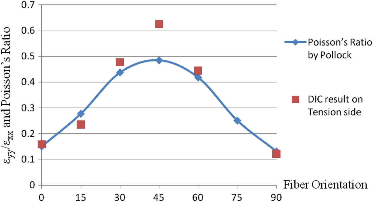

Concluding remarks

A combined specimen-fixture-mechanical loading system has been (a) developed with an integrated 3D-DIC measurement system, (b) used successfully to obtain the full-field deformation measurement for both tension side and compression surfaces of a small woven composite specimen undergoing combined compression–bending loading and large deformation and (c) used to study the nonlinear behavior of a woven glass/epoxy laminate undergoing compression–bending loading.

Experimental results for specimens undergoing both linear and highly non-linear deformations during monotonic loading clearly show the strong relationship of fiber angle to the global response variables, P−Δ and M_max−Δ. The critical strain concentration region on the compression bending specimen has been investigated for all fiber angles. The strain results show that the axial strain ɛ_xx along the longitudinal and transverse directions are generally non-uniform and a strong function of fiber angle. Similar results were measured for both the transverse strain ɛ_yy and shear strain ɛ_xy, as shown in Appendix A.

For the 0°/90° fiber orientations, the performance of the specimen approximates an orthotropic material, especially on the tensile surface of the specimen. When the orthogonal fiber directions do not align with the axial and transverse directions, the following observations are noted:

the corresponding distinct differences in the strain fields between the tension and compression surfaces at the critical location for different fiber angles is clearly related to the disparity in local material failure mechanisms between the tension (e.g. matrix cracking) and compression (e.g. fiber buckling) surfaces

the presence of anticlastic (double) curvature of the specimens in the critical region is strongly affected by the fiber angle, θ, with measured anticlastic curvature a monotonic function of fiber angle from 0° to 45° and relatively small for low fiber angles

the variations in measured Poisson's ratio between the tensile and compressive surfaces, as well as the variation in compression-side Poisson's ratio with width and axial position, are further evidence of the differences in failure mechanisms on the compression and tension surfaces.

Results from our studies indicate that the measured highly non-uniform deformation fields, especially in the critical regions, will be important in the development of physically based, damage/failure models that the investigators are currently studying.

Footnotes

Acknowledgement

The support of Dr. Hubert Schreier and Correlation Solutions, Incorporated through technical interactions regarding the optical measurements is gratefully acknowledged. Specimen preparation and manufacturing by Mr Bill Bradley and the College of Engineering and Computing Machine Shop is also acknowledged. Finally, the support of Mr Donald Martin at Norplex Micarta in providing all of the material used in the experiments is deeply appreciated by the authors.

Conflict of interest

None declared.

Funding

The support of the Air Force Office of Scientific Research and Dr David Stargel via grants # FA9550-09-1-0543 and financial support provided by the University Of South Carolina College Of Engineering are gratefully acknowledged.

a

This composite material is used as a structural material in computer boards.

b

A Q-basic program was used to evaluate the input/output process. The configuration of the handshake signal was determined to be “COM1:9600,N,8”, with a maximum refresh rate for each signal of 20 milliseconds.

c

Modern LED light systems or fiber optic light sources are recommended as a replacement for halogen lights, since the IR filters used to reduce heat generated by halogen lights can overheat and fail during extended operation.

d

For ± 45° fiber orientation, the specimen did not fracture even when end displacement exceeded 90% of its length, even though significant damage was visually evident (fiber buckling on compression side, extensive matrix cracking on both sides) at maximum displacement.

e

For all fiber orientations, each strain component in the critical region is obtained by averaging the strain values within a 5 mm diameter region that is centered at the specimen mid-span and mid-width.

f

Since the specimen is loaded in a nominally symmetric manner relative to a Y-Z plane located at the specimen centerline, data is provided for one-half of the specimen length.

References

Sun

Chen

. A simple flow rule for characterizing nonlinear behavior of fiber composites. J Compos Mater 1989; 23: 1009–1020.

Sun

Yoon

. Elastic–plastic analysis of AS4/PEEK composite laminate using a one-parameter plasticity model. J Compos Mater 1992; 26: 293–308.

Kenaga

Doyle

Sun

. The characterization of boron/aluminum composite in the nonlinear range as an orthotropic elastic–plastic material. J Compos Mater 1987; 21: 516–531.

Chen

Sun

. A plastic potential function suitable for anisotropic fiber composites. J Compos Mater 1993; 27: 1379–1390.

Tamužs

Andersons

Sparnins

. Response of cross-ply composite to off-axis loading. J Compos Mater 2002; 36: 2125–2134.

Tamuž

Andersons

Aniskevic

. Creep and damage accumulation in orthotropic composites under cyclic loading. Mech Compos Mater 1998; 34: 321–330.

Odegard

Searles

Kumosa

. Nonlinear analysis of woven fabric-reinforced graphite/PMR-15 composites under shear-dominated biaxial loads. Mech Compos Mater Struct 2000; 7: 129–152.

Ogihara

Reifsnider

. Characterization of nonlinear behavior in woven composite laminates. Appl Compos Mater 2002; 9(4): 249–263.

Tamuzes

Dzelzitis

Reifsnider

. Fatigue of woven composite laminates in off-axis loading I. The mastercurves. Appl Compos Mater 2004; 11(5): 259–279.

10.

Xing

Reifsnider

Huang

. Progressive damage modeling for large deformation loading of composite structures. Compo Sci Technol 2009; 69(6): 780–784.

11.

Yang

Kozey

Adanur

. Bending, compression, and shear behavior of woven glass fiber-epoxy composites. J Compos: Part B 2000; 31: 715–721.

12.

Van Paepegem

Degrieck

. Experimental set-up for and numerical modeling of bending fatigue experiments on plain woven glass/epoxy composites. J Compos Struct 2001; 51: 1–8.

13.

Quek

Waas

Shahwan

. Failure mechanics of triaxially braided carbon composites under combined bending-compression loading. J Compos Sci Technol 2006; 66: 2548–2556.

14.

Wisnom

Atkinson

. Constrained buckling tests show increasing compressive strain to failure with increasing strain gradient. J Compos Part A 1997; 28: 959–964.

15.

Sutton

Wolters

Peters

. Determination of displacements using an improved digital correlation method. Image Vision Comput 1983; 1(3): 133–139.

16.

Peters

WH III

Ranson

Sutton

. Application of digital correlation methods to rigid body mechanics. Opt Eng 1983; 22(6): 738–743.

17.

Bruck

McNeill

Sutton

. Determination of deformations using digital correlation with the newton-raphson method for partial differential corrections. Exp Mech 1989; 29(3): 261–267.

18.

Luo

Chao

Sutton

. Application of stereo vision to 3-D deformation analysis in fracture mechanics. Opt Eng 1994; 33(3): 981–990.

19.

Luo

Chao

Sutton

. Accurate measurement of three-dimensional deformations in deformable and rigid bodies using computer vision. Exp Mech 1993; 33(2): 123–133.

20.

Helm

McNeill

Sutton

. Improved 3-D image correlation for surface displacement measurement. Opt Eng 1996; 35(7): 1911–1920.

21.

Helm

Sutton

McNeill

. Deformations in wide, center-notched, thin panels: part I: three dimensional shape and deformation measurements by computer vision. Opt Eng 2003; 42(5): 1293–1305.

22.

Helm

Sutton

McNeill

. Deformations in wide, center-notched, thin panels: part II: finite element analysis and comparison to experimental measurements. Opt Eng 2003; 42(5): 1306–1320.

23.

Sutton

Orteu

Schreier

. Image correlation for shape, motion and deformation measurements, New York: Springer, 2009, pp. 10013–10013.

24.

Willems

Lomov

Verpoest

. Optical strain field in shear and tensile testing of textile reinforcements. J Compos Sci Technol 2008; 68: 807–819.

25.

Giancane

Panella

Nobile

. Fatigue damage evolution of fiber reinforced composites with digital image correlation analysis. J Procedia Eng 2010; 2: 1307–1315.

26.

Sutton

Yan

Tiwari

. The effect of out-of-plane motion on 2D and 3D digital image correlation measurements. Opt Lasers Eng 2008; 46: 746–757.

27.

Correlated Solutions, Incorporated, www.correlatedsolutions.com, 2009–2013.

28.

Pollock P, Yu L-Y, Sutton MA, et al. Full-field measurements for determining orthotropic elastic parameters of woven glass-epoxy composites using off-axis tensile specimens, experimental techniques. Epub ahead of print 12 June 2012. DOI: 10.1111/j.1747-1567.2012.00824.x.

29.

Sutton

Yan

Deng

. 3D digital image correlation to quantify deformation and COD in ductile aluminum under mixed-mode I/III loading. Opt Eng 2007; 46(5): 051003–1–051003-17.

Development and application of an experimental system for the study of thin composites undergoing large deformations in combined bending–compression loading

Abstract

Keywords

Introduction

Experimental considerations

Composite test specimens and preliminary studies

Integrated stereovision and compression–bending loading systems

Tinius Olsen 5000 loading frame

Specimen grips

Control system

Four-camera stereovision system

Lighting

DOF and FOV

Camera positioning and orientation

Speckle patterning

Calibration

Measurements

Experimental results and discussion

Axial load and centerline moment versus axial displacement

Surface strain measurements

Strain Localization, θ = 0° and 45°

Anticlastic curvature

Strain variations for small and large compressive displacement

Axial Strain Field

Fiber direction strains and axial–transverse direction strains in critical region

Poisson's ratio

Concluding remarks

Footnotes

Acknowledgement

Conflict of interest

Funding

a

b

c

d

e

f

References