
Abstract
Although composite materials have numerous advantages, some disadvantages, including high manufacturing costs, are relevant. In particular, if the material is applied to large structural components, such as the wings, flaps or fuselage of an airplane, efficient manufacturing processes are required to generate products that are both high quality and cost effective. Therefore, monolithic designs often become integral due to the lower overall part count and simplified designs (e.g. reducing the number of joints and fasteners significantly). For highly integrated monolithic structures, developing a robust manufacturing process to produce high quality structures is a major challenge. An integral structure must conform to the tolerance requirements because those requirements may change. Process-induced deformations may be an important risk factor for these types of structures in the context of the required tolerances, manufacturing costs and process time. Manufacturing process simulations are essential when predicting distortion and residual stresses. This study presents a simulation method for analysing process-induced deformations on the structure of a composite multispar flap. The warpage depends on the thermal expansion and shrinkage of the resin. In this study, a sequentially coupled thermo-mechanical analysis of the process will be used to analyse temperature distribution, curing evolution, distortion and residual stresses of 7.5 m long composite part.
Keywords
Introduction
High-performance carbon fibre-reinforced composite materials are widely used in aerospace structures because they have many advantages: they are lightweight, have high stiffness and strength and are very durable. To attain the full potential of these materials, the disadvantage, including the relatively high material and manufacturing costs, must be weighed against the advantages. Monolithic designs often become integral to lower manufacturing costs and to realise a composite-based design, reducing the manufacturing costs with lower overall part counts and simplified designs (e.g. reducing the number of joints and fasteners). For highly integral monolithic structures, developing robust manufacturing processes that produce high quality structures remains a major challenge. The development of stable production processes for large integral composite parts, such as flaps, wings or fuselage sections, is complex and fraught with risk. These risks are driven by the distinctive features of composite materials under the influence of the manufacturing process. Because matrix material epoxy resin is a thermoset polymer, it is frequently used. Due to the stringent requirements of the aerospace industry, toughened, thermally stable resin systems are preferable. Typically, resin systems with a high curing temperature (approximately 180℃) are chosen to achieve glass transition temperatures above 160℃. While curing carbon fibre-reinforced polymer (CFRP) materials, the inhomogeneous material properties facilitate the development of process-induced deformations and stresses due to the chemical matrix shrinkage and thermal expansion. The properties of the resulting material will be influenced by the process-dependent deformations and stresses. In fact, the internal stresses may become intense enough to cause fibre matrix debonding, matrix failure or delamination. In general, defects on the micro scale, such as matrix fibre debonding or small matrix cracks, are barely measurable and only noticeable through the reduced stiffness or strength properties. On the macro scale, creating the wrong dimensions in the resulting shape is one of the main risks. For large structures, redesigning a production facility with regard to the moulds, jigs and tools is time consuming and expensive.
Simulating manufacturing processes is essential when evaluating the correct process parameters to predict the distortion and residual stresses. In this paper, a simulation strategy will be presented and compared to the middle-sized production of an integral composite multispar flap (CMF). The flap is 7.5 m long and is done using a one shot resin transfer moulding (RTM) process. Various different processes are available to manufacture thermoset fibre-reinforced composite parts. In general, a process that uses prepeg (premixed fibre and high viscosity matrix systems) is distinguishable from a process using dry textiles impregnated via infusion (vacuum driven) or injection (pressure driven). These processes are called liquid composite manufacturing (LCM) and can be classified as open mould techniques, such as the resin transfer injection (RTI), or closed mould techniques, such as resin transfer moulding (RTM) (Figure 1). To reach high fibre volume contents, accelerate injection times and minimise the amount of voids, additional pressure is applied. The RTM process has a heating system that can be applied with a heating press, consuming as little energy as an autoclave.
RTM process.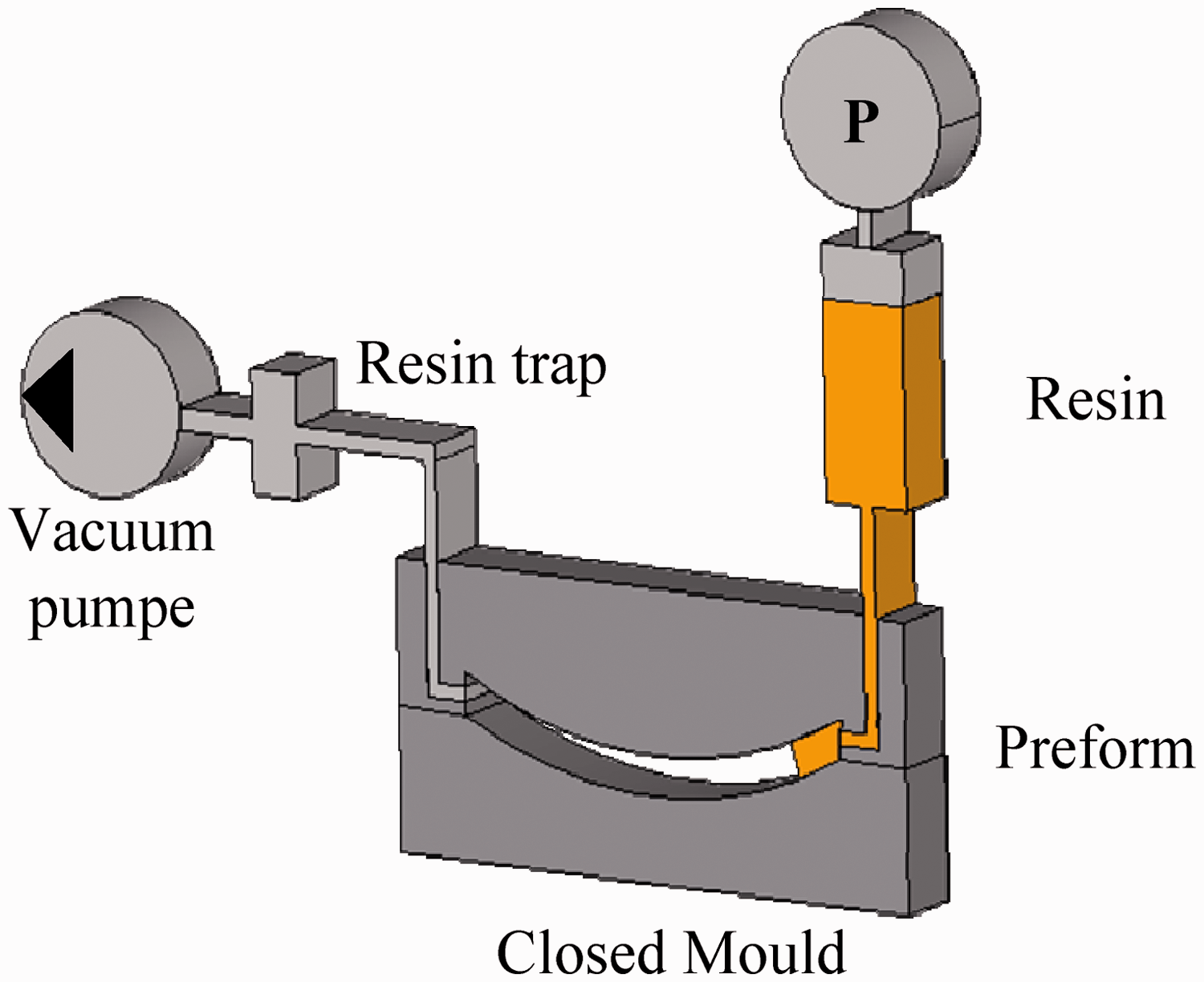
Therefore, RTM is suitable for mass producing high quality parts while minimising manufacturing costs. In the following work, the simulation methods will focus on RTM and the materials used during this process.
The composite part is cured using a one shot process. Dry textile forms are placed into a mould, heated to the injection temperature (120℃), injected, heated to the curing temperature (180℃), cured for 2 h and finally cooled to room temperature. While curing, the thermoset resin passes through three different morphological states (Figure 2). The resin converts from a liquid (i) to a rubbery state (ii) and, finally, to a solid state (iii). These changes are gradual, but from an engineering point of view, the transition can be defined as the gel point (liquid to rubbery) and the vitrification point (rubbery to solid). A model must reflect these important changes.
Curing process.
In general, three types of analysis can be identified: elastic models, incrementally elastic models and viscoelastic models. Elastic models account for the anisotropic coefficients of thermal expansion while neglecting the effects of the curing reaction, chemical shrinkage, and viscoelastic material properties; these models are fast, but not reliable. Incrementally elastic approaches can be found in the literature; these methods model the resin modulus development, depending on the degree of cure, through either linear, incremental linear 5 or nonlinear approaches.17–19 These models are more complete, but neglect the viscoelastic material behaviour and the effects of relaxation. To represent the true residual stress state, a viscoelastic approach that depends on the degree of cure, the temperature and the time is necessary; examples are reported by Svanberg et al., 4 Prasataya, 22 Kim and White 11 and Zoberiy. 7
In this study, a manufacturing process simulation is presented that begins with a thermodynamic analysis and ends with a sequentially coupled mechanical analysis used to examine the warpage generated during a RTM process in a 7.5 m composite part. The entire curing process is simulated using a transient thermodynamic analysis to determine the temperature inside the mould and the part. During this step, the degree of cure is computed by implementing a user routine that applies an exothermic heat flux from the chemical curing reaction. Afterwards, the temperature results are applied to a transient mechanical analysis. During the mechanical analysis, the material was treated as a linear viscoelastic material dependent on the degree of cure, temperature and fibre volume content; this analysis was implemented via a user subroutine into the implicit Finite Element code, Samcef/Mecano.
Simulation strategy
The manufacturing process for composite parts is a multi-physical problem because it connects the thermodynamic discipline (thermal conduction in the moulds and parts), chemistry (resin curing) and mechanical analysis (warpage). Additionally, this multi-physical problem is compounded with a multi-scale problem because single components, such as resin, fibre and fabric, are combined and used to build large structures, including wing covers, fuselage sections, etc. This analysis method should represent the correct physical behaviour on the part level while using the involved parameters to perform parameter studies, sensitivity analyses and parameter variability analyses to increase the part quality, decrease the manufacturing costs and design stable manufacturing processes. Therefore, a simulation strategy that generates a detailed analysis with less computational effort is required.
Two different solutions are available for the multi-physical problems between thermo and mechanical analyses. First, a strong coupling is possible; therefore, the thermal and mechanical equations are solved simultaneously. Second, there will be a sequential coupling; a thermal analysis is performed, and temperature profiles are transferred as boundary conditions, specifically temperature loads, to the mechanical analysis. This sequential coupling can be performed if the thermal analysis influences the mechanical portion, but not the inverse. In the given case, the mechanical part does not produce any type of heat; therefore, a sequential coupling is sufficient. This coupling generates different advantages because optimising the temperature process parameters, such as the heat rate, curing temperature and curing time, in the thermal portion can be performed separately. In the mechanical portion, parameter studies, such as the variations in the laminate stacking, the influences of the draping errors and the variations of the fibre volume content, can be analysed without recalculating the temperature loads when the temperature is only slightly affected. The sequential coupling enables the use of different meshes and elements in the different analysis modules. For the RTM process, the mould and part must be analysed during the thermal analysis process using a volume mesh for the mould and the part (Figure 3). In the mechanical portion, the deformation and stress of the mould are not necessary. Therefore, shell elements may be used, reducing the computational effort significantly; varying the layup can be performed easily without changing the geometry.
Simulation strategy.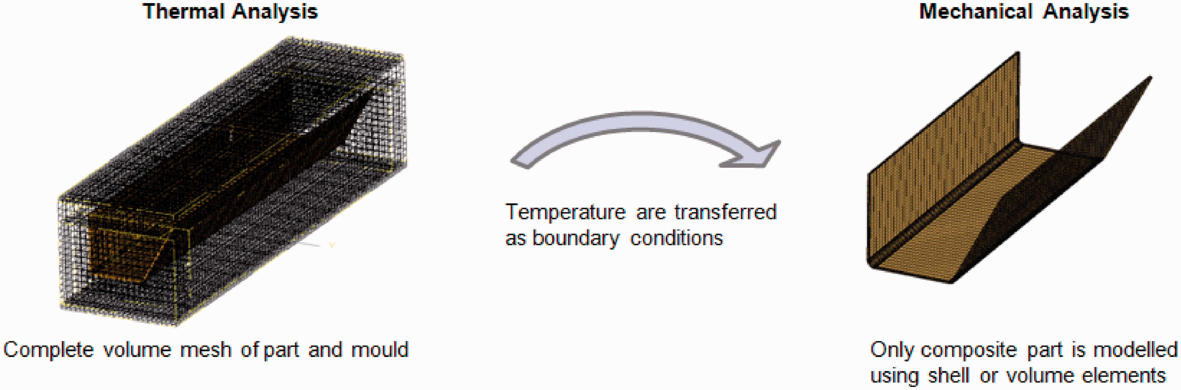
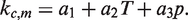
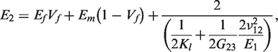
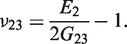
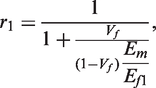
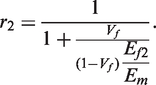
To capture the multi-scale problem, the following method is recommended. While manufacturing composites, the fibre volume content can be influenced, deviating from the ‘As-Planned’ to the ‘As-Built’ value. Depending on the fibre volume content, all properties change. To account for possible variations in the fibre volume content and resin properties, the homogenised ply properties must be recalculated during the transient analysis. Two general approaches can be applied by using a numerical unit cell/representative volume element approach or by using analytical homogenisation methods. Using the numerical unit cell method leads to a two scale analysis that is computationally wise but more expensive. Consequently, the analytical approach is preferred. Using an analytical micromechanical homogenisation method changes the following parameters. The advantage of this approach is that the input parameters can be divided into the resin and fibre properties. Experimental characterisation of single quantities is always easier, as was demonstrated by the researchers in Ref. [23]. Another advantage is that the method will provide additional results because cured homogenised properties on the ply level will be available. Therefore, the following material properties are provided: Young’s moduli E1, E2 and E3, shear moduli G12, G23 and G13, Poisson's ratios v12, v13 and v23, thermal expansion coefficients CTE1, CTE2 and CTE3, heat capacity cp, density ρ and thermal conductivities
Thermal analysis module
The necessity of performing a heat transfer analysis in the composite part is related to two different factors. The first factor depends on the thickness of the laminate. For thin laminates, assuming a uniform temperature in direction of the thickness is valid because exothermic reaction heat can be neglected. The second aspect is a temperature gradient within the part itself. Due to the forced convection heating, the curing process is much faster where the temperature is higher. Using a rough rule-of-thumb, increasing the temperature by 10℃ doubles the speed of the curing reaction. To apply the exothermic heat flux from the resin cure reaction, a model developed by Bogetti and Gillespie
2
is used. The governing equation for heat transfer is the transient anisotropic heat conduction equation containing a heat flux generation term from the exothermic cure reaction
Cure kinetics
Thermoset resins transform from a liquid state to a solid state at elevated temperatures, and their curing processes can be described using generalised empirical rate equations or mechanistic models. Mechanistic models begin to describe the curing process on an atomistic scale via descriptions of the growing macromolecules. The empirical rate approach derives a phenomenological mathematical description of the curing process from experimental studies using differential scanning calorimetry (DSC). With this method, the exothermic heat flow is measured and interpreted while assuming that this heat flow is proportional to the degree of cure. The reaction kinetics are often used to describe a reaction of nth order; p represents the conversion factor/degree of cure (varying from 1 to 0) and describes its development. The temperature dependence is described using the Arrhenius rate constant ki
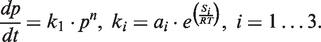
The Arrhenius term is based on the material and process parameters with the thermal activation energy of the reaction Si, the universal gas constant R, and the temperature T. The kinetic reaction models available in the literature for different resin systems are diverse. In general, the model must accommodate different curing situations, particularly the variation in isothermal and dynamic temperature conditions.
Kamal and Sourour developed a model that is mostly used for the given resin system (RTM6)
3
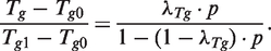
Glass transition temperature
While curing epoxy resin, three different morphologic states will be passed. The resin will be converting from liquid to rubbery and to solid states. These changes are not defined as points, but from the engineering perspective, they will be defined as points and connected to the glass transition temperature. The changes in the glass transition temperature depend on the degree of cure. These changes can be accounted for using equations available in the literature
6
Specific heat capacity
The heat capacity varies with the degree of cure and the reaction temperature; this attribute is also one of the sensitive parameters used to describe the thermal behaviour of thermoset resin. The specific heat increases with the temperature, but it decreases when changing from a liquid to a solid state. This dependency is non-linear. The change from a liquid to a solid will be approximately 15–20% and generates a direct error in the idealisation of the thermal material behaviour. Therefore, the dependence of the specific heat capacity on the temperature and degree of cure must be considered. There are different approaches towards idealising these dependences; one approach comes from Balvers.
9
He defined
For
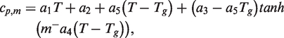
For
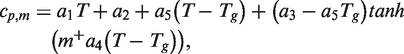
The heat capacity is a scalar quantity and is not influenced by the type of fabric or arrangement of the fibres. The following approach was reported by Schürmann
13
and used by Johnston
5
Thermal conductivity
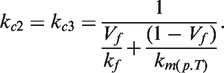
The thermal conductivity changes with the temperature and the degree of cure, similar to the heat capacity. However, the thermal conductivity is a vector quantity. Three values must be assumed. For the pure resin, an isotropic material behaviour may be defined, and all thermal conductivity parameters can be equalised. There are also excising approaches used to model thermal conductivity. Johnston models the thermal conductivity as a function of the degree of cure and temperature
The thermal conductivity of a composite will be a first order tensor that strongly depends on the type of fabric/unidirectionality of the fibre arrangement. Analytical mixing rules for unidirectional fibre arrangements are based on the theory of parallel adjustment in the thermal conductivity in the fibre direction and a series connection in transverse direction of the fibre. For a unidirectional layer, an orthotropic/transverse isotropic behaviour can be observed in the thermal conductivity. Extended versions of this model have been published by Kulkarni et al.14 and Springer and Tsai15

Mechanical analysis module
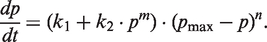
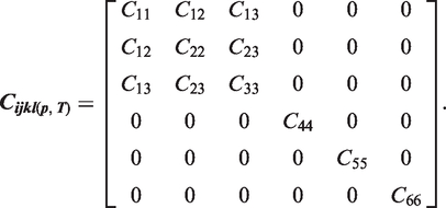
The mechanical module should capture the relevant variations in the material parameters to represent the behaviour of the material. This material can be idealised as an orthotropic material with nine relevant material parameters. The second derivative of the deformation energy through the deformation is the material tensor and can be written as follows
The major indicators for process-induced deformations are chemically and thermally induced strains. Therefore, an incremental formulation of the strains is defined and added to the mechanical strain

The chemically induced strains are based on the increments of the degree of cure. The total value of this vector quantity is the computed homogenisation approach in equations (18)–(27)
A similar approach is applied to the thermally induced strains and is based on the presented homogenisation approach (equations (31)–(33))
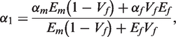
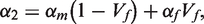
To account for the variation in the resin properties, homogenisation methods can be applied. The micromechanical approaches used to homogenise the Young’s moduli are mostly analytical rules for mixtures based on the application of the Voigt model in fibre direction and the Reuss model transverse to the fibre direction. The Voigt model is derived from the examination results; the fibre and the matrix can be treated as a parallel connection of springs. The Reuss model applies a serial connection between the fibre and matrix stiffness. Using these approaches, the following basic restrictions must be fulfilled. The lamina must be macroscopicly homogeneous, linearly elastic and initially stress free. The fibres are homogeneous, linear elastic, isotropic, regularly spaced and perfectly aligned. The matrix must be homogeneous, linearly elastic and isotropic. 24 Restrictions such as the initial stress-free condition for the lamina and the linearly elastic behaviour for the resin are not fulfilled. Additionally, the fibre volume ratio changes due to thermal expansion and shrinkage. The magnitude will be approximately 2–3%. This dilemma might be solved by computing the homogenised properties incrementally. As expected, the composite transverse moduli are highly dependent on resin behaviour, while the fibre direction properties were far less affected. In the literature, different micromechanical approaches for the transverse properties are available.
As shown in Figure 4, the differences between the approaches are quite pronounced, particularly for high fibre volume ratios. The maximum value for squared fibre packing is approximately 0.785, and that for hexagonal packing is 0.90. After analysing the different approaches, the Hashin/Hill approach estimates the highest values for the transverse Young’s modulus. In this study, the Hashin/Hill homogenisation approach was chosen because a consistent approach for a transverse isotropic material exists (equations (18)–(27)). This approach is valid for a certain material range but must be proved for the materials used in this study. Hashin/Hill defined first the hydrostatic fibre and matrix modulus
Comparison between the different analytical homogenisation approaches for the transverse module.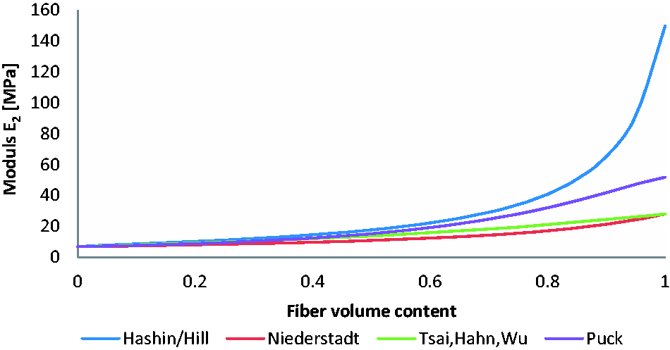
These values are used to determine the lateral bulk modulus
For an orthotropic material, nine elastic coefficients may be successively derived from the following equations

For transverse isotropy (which will be used in this study), the following assumptions can be found

Similar to the engineering constant, the thermal expansion coefficients (CTE) (
In the transverse direction, the thermal expansion of the compound is matrix dominated. The theoretical fundament base is connected in series. Using the assumption that the CTE of the matrix is not cure-dependent, a micromechanical model can be defined in the simplest way. In the transverse and longitudinal directions, the following approaches from Schürmann
13
are chosen

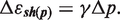
To determine the influence of chemical shrinkage, a chemically induced shrinkage coefficient (CSC)


The viscoelastic relaxation effects must be used and cannot be neglected. A possible approach using the incrementally written differential form of the relaxation, as discovered by Zocher et al.
16
and Svanberg and Holmberg
4
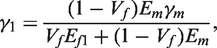
, can be used. To account for this effect, an instantaneous viscous elastic approach is applicable. Therefore, to define the stress at the actual time, a relaxation term can be added using a formulation based on a Maxwell element

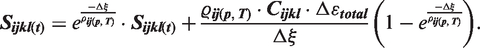
The parameters The global viscoelastic behaviour is based on the matrix component The fibres have a pure linear elastic behaviour Homogenisation methods can be used to relate the matrix relaxation behaviour to the composite behaviour.
Therefore, the relaxation behaviour can be characterised as a pure resin that displays isotropic behaviour. This isotropic material can be described using the
Material characterisation
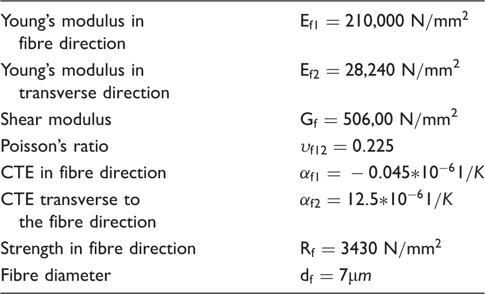
Fibre properties.
Matrix properties (cured).
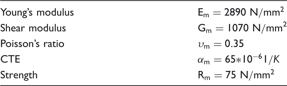
The present study concentrates on a polyfunctional epoxy resin (RTM 6) supplied by Hexcel Composites (UK). The resin is used to manufacture aircraft composite structures via the RTM process and is currently receiving considerable attention from civil aircraft manufacturers. The composition of the resin system includes two aromatic diamine hardeners. The expected service temperatures of final products range from −60℃ to 180℃. At room temperature, RTM 6 is a translucent paste, but its viscosity drops very quickly after heating. The uncured resin has a density of 1.117 g/cm3, and the fully cured resin has a density of 1.141 g/cm3. The recommended cure regime for this resin is 160℃ for 75 min, followed by a post-cure treatment at 180℃ for 2 h, generating the expected glass transition temperature (approximately 183℃) in the cured material. The recommended curing process (180℃ for 120 min) generates a 196℃ glass transition temperature and a final degree of cure of approximately 96%. The following resin properties are given for the cured material (table 1 and 2).
Application to a test case
Experimental test setup
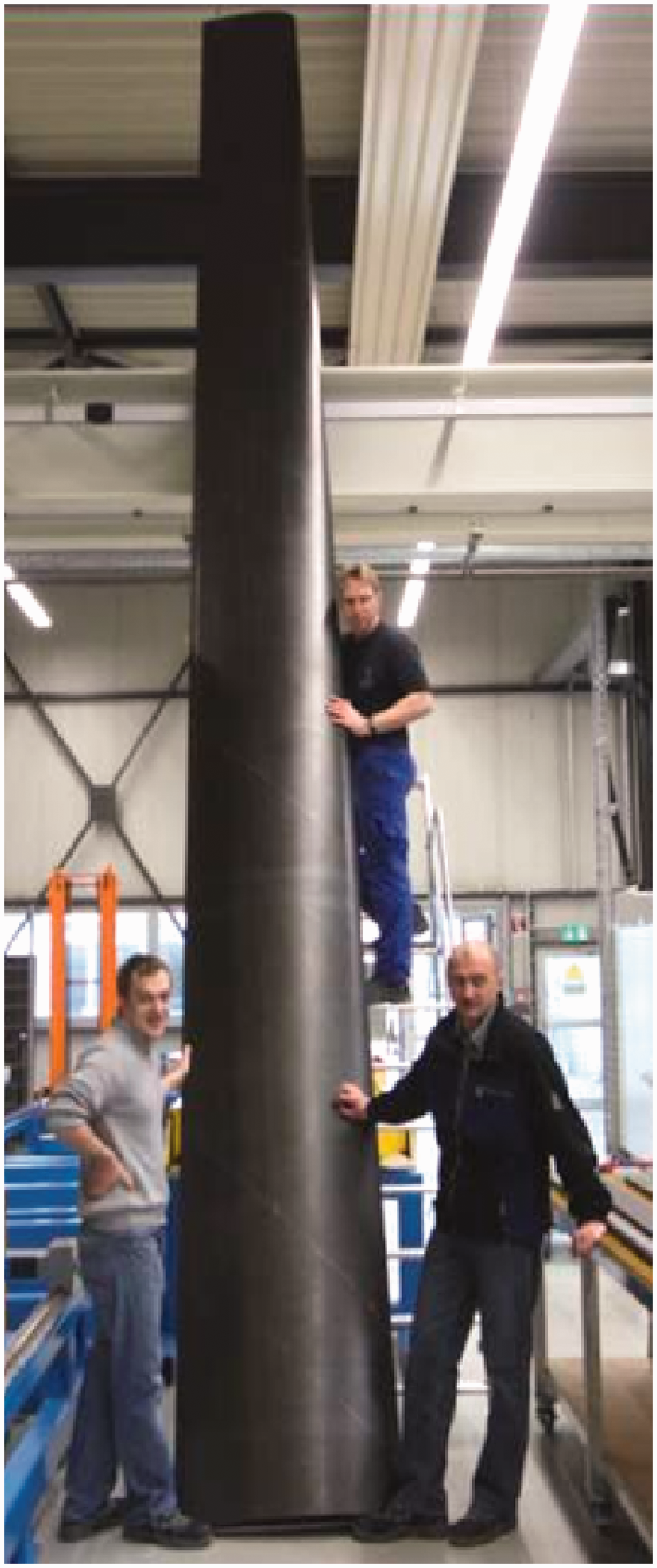
The objective of this study was to apply the simulation method to analyse the manufacturing process of an integral one shot RTM CMF. The test structure has the length of 7.5 m (Figures 5, 6 and 7). The application of the analysis method on this middle-sized structure presents the application possibilities using parameter studies on process parameters to reduce process time, to evaluate risk parameters and their influence and to improve part quality.
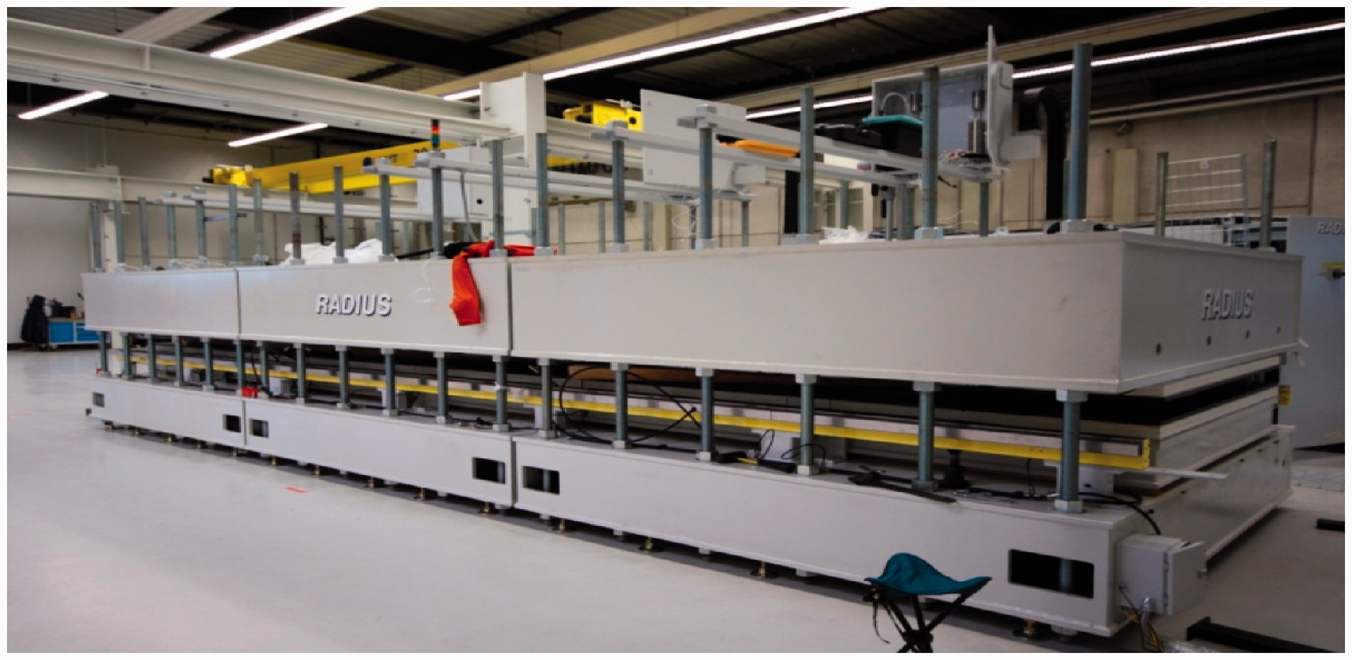
Cross section of the composite part. Heat press and mould. Composite part.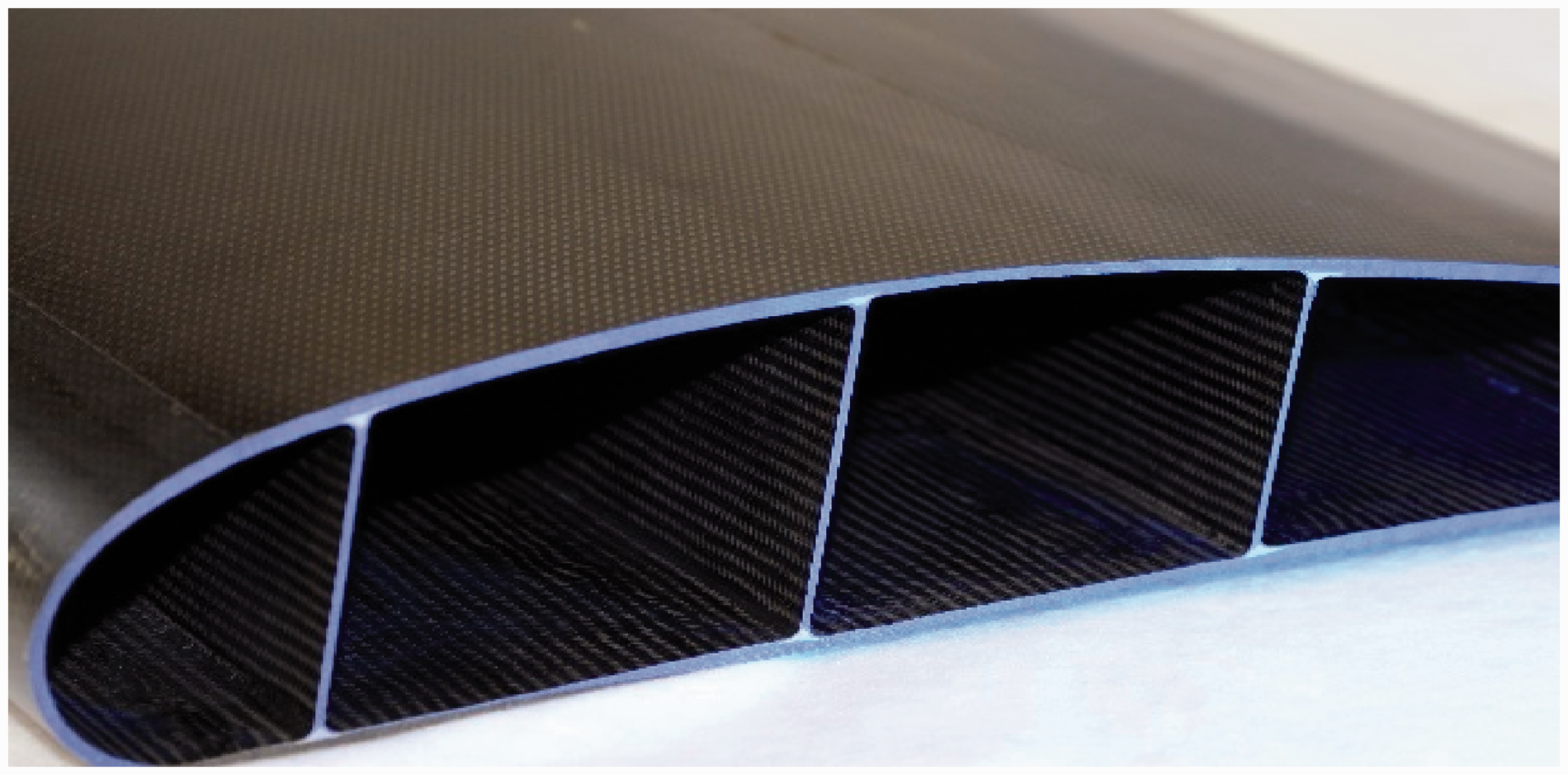
Numerical analysis
Starting from an imported CAD model, the FE model was built with a volume mesh using 985640 tetrahedral volume elements for the thermal analysis portion of the sequential coupled analysis. The complete mould and the composite are meshed with volume elements (Figure 8).
FE discretisation mould for the thermal analysis.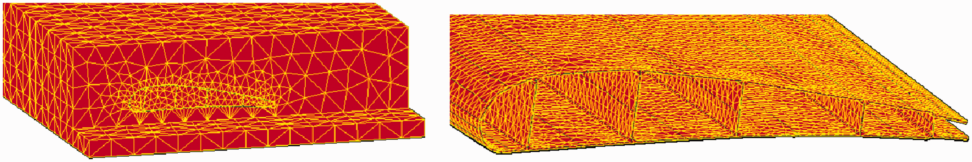
For the boundary conditions, a temperature profile (Figure 9) was applied to the upper and lower sides of the mould. On the sides of the mould, a natural convection was applied with a convection coefficient of 12 W/m2 and a fluid temperature of 20℃.
Temperature boundary conditions and infusion point.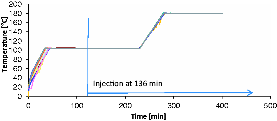
The mechanical FE model of the flap was simplified to a shell structure. The laminate stacking is made of a quasi-isotropic laminate that contains different types of satin weave fabric (Hexcel G0926). Every fabric ply (0/90) was modelled using four unidirectional plies (0/90/90/0). The model of the multispar flap was simplified to the shell structure presented in Figure 10.
FE discretisation for the composite portion of the mechanical analysis.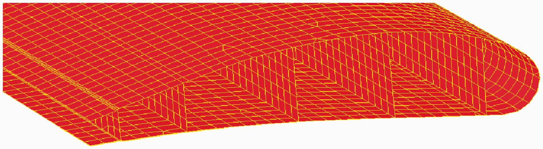
The mesh of the flap consists of 1984 (8%) triangle and 23028 (92%) quadrangle multilayer linear shell elements when using a Reissner Mindlin approach.
Results
In the following, the results of the thermal and mechanical analyses are presented. For the thermal analysis module, the temperatures inside of the composite part and mould are displayed in Figure 11. The points are arbitrarily chosen. The dashed lines represent the nodal temperatures in the spars, while the continuous lines indicate the nodal temperatures in the skin.
Temperature boundary conditions and temperature inside the composite part/mould.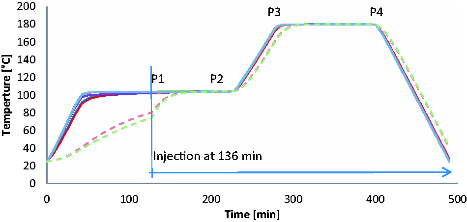
Figure 11 displays the temperature evolution during the process. At the beginning of the process, the thermal conductivity of the dry preform is four times lower and is visible during the slow heating portion of the temperature curves for the spars. After reaching the injection point, the resin properties are added, as well as the thermal conductivity, heat capacity and density change. After this point, the thermal conductivity is dictated by the resin and fibres. The heating is much faster and more uniform. In the following pictures, the temperatures in the mould, in the mandrels and on the composite parts are presented at point 3 (280 min).
The simulation shows that the temperature distribution in the mould is not homogeneous (Figures 12–14). During the heating from the injection temperature to the curing temperature, the composite part temperature varied largely. The skin parts are heated quickly, but the mandrels heated slowly, delaying the heating process for the spars. The temperature has a strong influence on the curing process (Figure 15) because that process is autocatalytic.
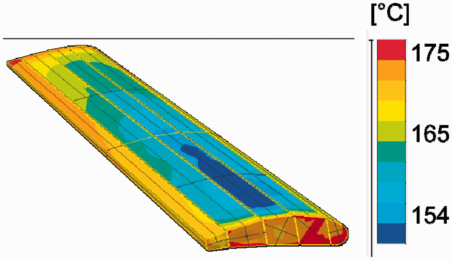
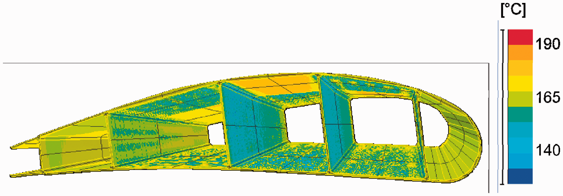
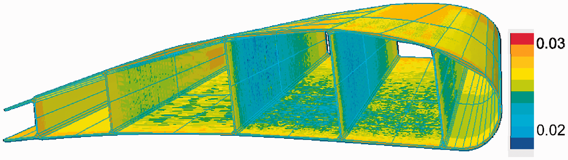
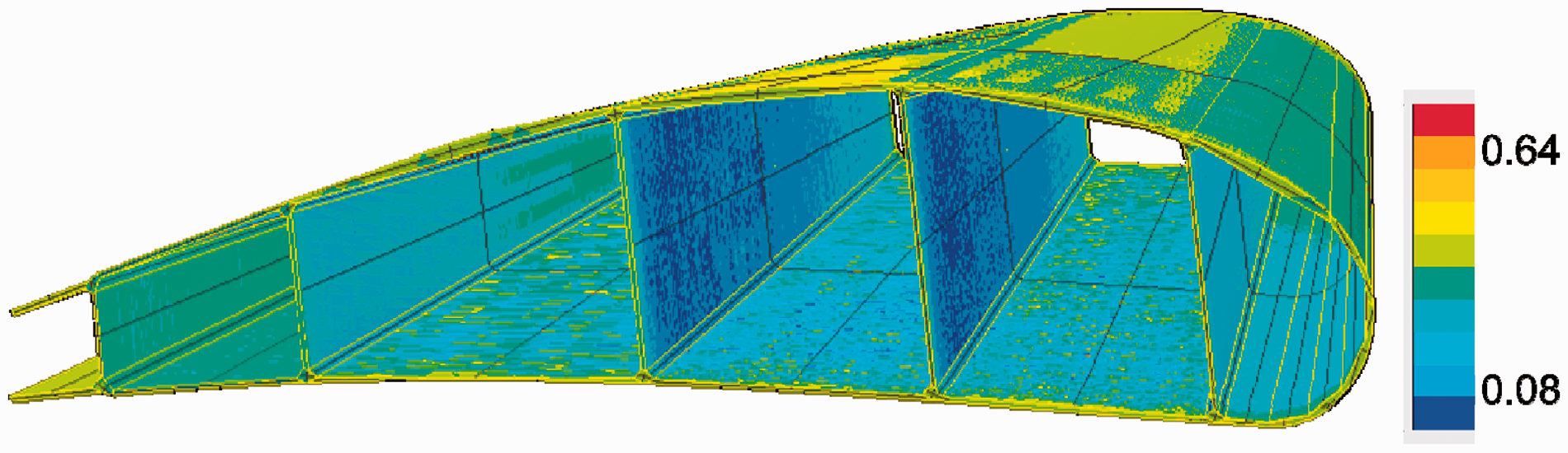
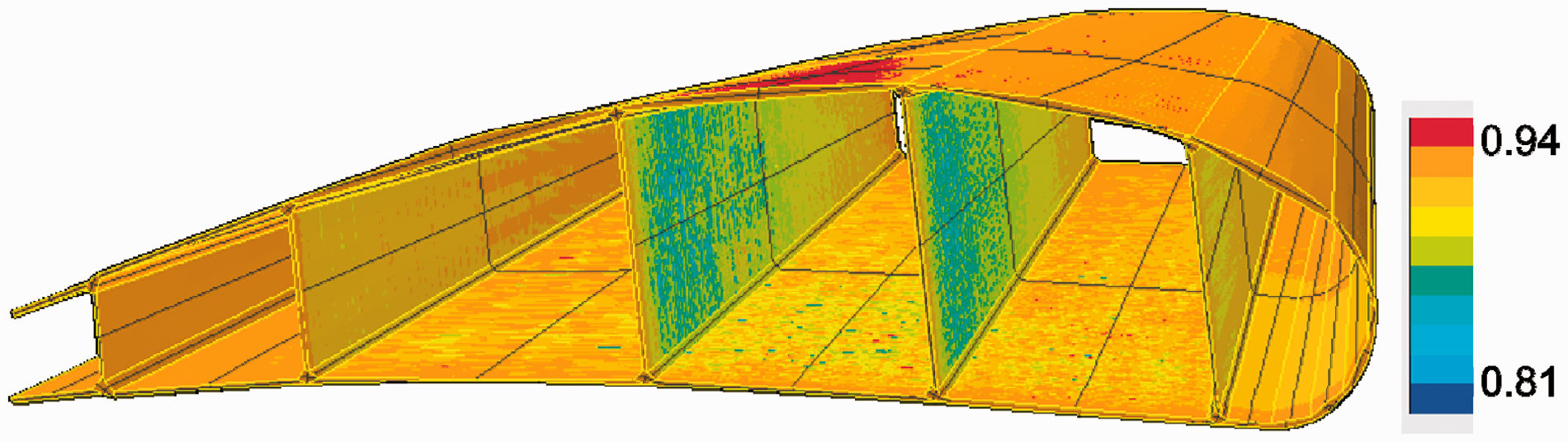
Temperature in the mould on a cross section located at the middle of the mould (max 190℃, min. 140℃). Temperature in the mandrels (max 175℃, min. 154℃). Temperature in the composite (max 190℃, min. 140℃) at 280 min after reaching 180℃. Press temperature and curing development in the composite part (min–max values). Press temperature and changes in the glass transition temperature in the composite (min–max values). After 227 min (before heating from 104 to 180℃) – degree of cure 0.01–0.03. After 278 min (after reaching 180℃) – degree of cure 0.08–0.64. After 310 min (middle of curing phase) – degree of cure 0.81–0.94.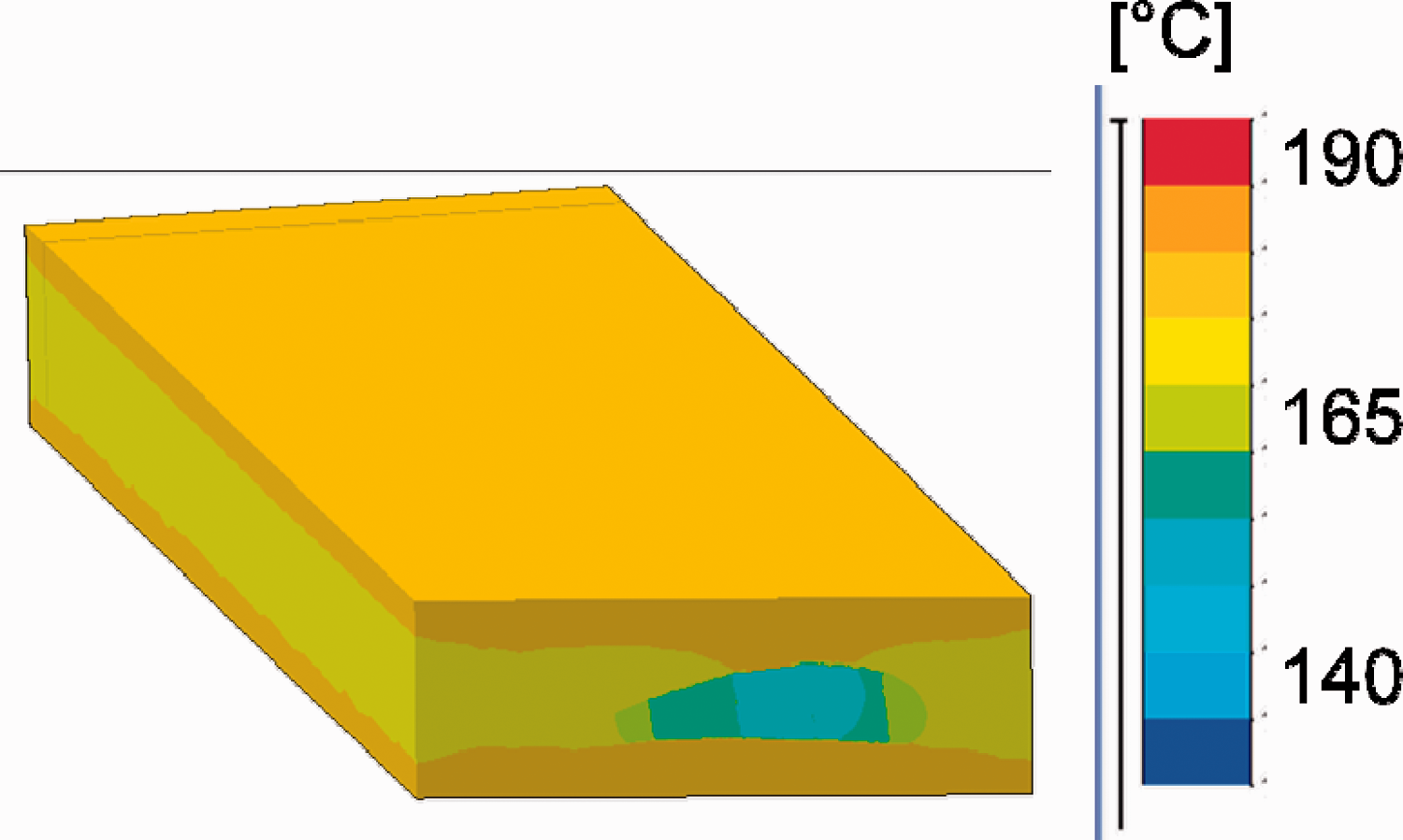
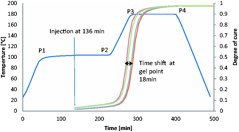
The curing development is shown at different points in the upper skin, the lower skin and the spars. The curing process is not homogeneous because it is sensitive to the non-uniform temperature fields. Figure 15 can be used to identify the first transition point (the gel point) from the liquid to the rubber state. The gel point was taken from the experimental characterisation (0.4). During the process, the gel point is delayed by 18 min. In Figure 16, the changes in the glass transition temperature are shown.
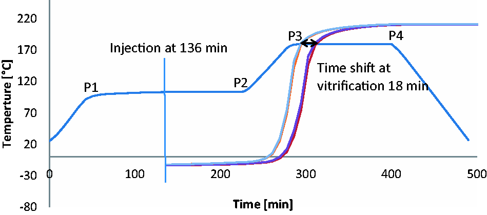
The glass transition temperature is coupled to the curing reaction using the DiBenedetto equation. Figure 16 can be used to identify the next transition point; this point is called the vitrification point and it is where the material transforms from a rubber phase to a solid phase. The vitrification point occurs where the glass transition temperature is higher than the local temperature. Therefore, this point is a process-dependent value. The time shift in the vitrification point is approximately 18 min. Figures 17–20 show the degree of cure at discrete time steps across the full structure.
After 400 min (after cooling) – degree of cure 0.98–0.98.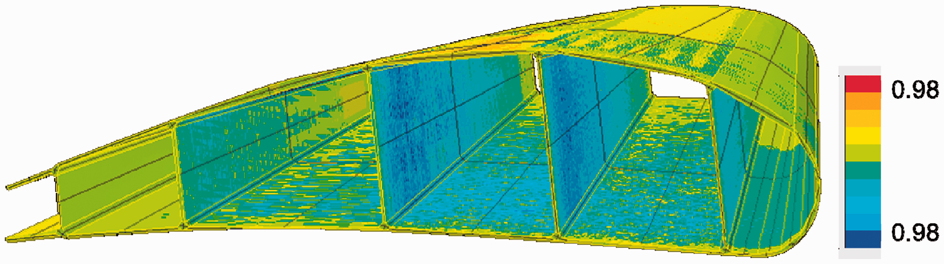
After analysing the curing evolution, the curing begins before reaching 180℃ in the skin region. The spars are cured at the end. The curing is very in homogeneous and dependent on the non-uniform temperature distribution.
The material model can provide a virtual material characterisation on the ply level. These results are presented as follows. The topology of the FE model is built on the ‘As-Built’ configuration that accounts for different discrete distributions of the fibre volume contents. The distribution of the fibre volume content is based on variations in the cavity and has been measured using the skin thickness. These changes are continuous. In the FE model, they are implemented as discrete steps between the spars and through eight sections from the inboard to the outboard side. Figure 21 presents the distribution based on the measured skin thickness. Additionally, the fibre volume content is in the modelled material and is influenced by the thermal and chemical shrinkage.
Resulting fibre volume content with variations from 0.63 to 0.46 based on thickness measurements.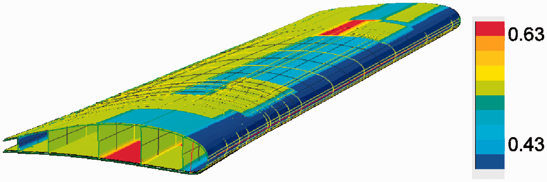
The ‘As-Planned’ fibre volume content is approximately 0.55. The variation in the fibre volume content starts with a minimum value (0.43) at the leading edge, while the maximum (0.63) occurs on the lower skin side. These variations significantly influence the resulting material properties, leading to a non-uniform distribution of material parameters in the structure. Figure 22 displays the changes in the thermal conductivity over the process time.
Changes in the thermal conductivity of the resin (kr) and laminate in the X (kx) and Y (ky)directions.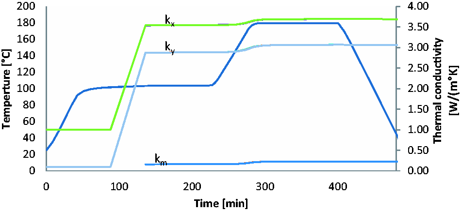
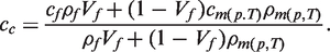
Figure 22 shows the changes in the thermal conductivity of the resin and the homogenised laminate values. For the laminate, the homogenised values are presented in direction of the global X and Y coordinates. The detailed observations in chapter 3 and 4 indicate that. The changes based on the degree of cure are smaller, particularly on the laminate level. The resulting cured values of the laminate are 3.70 W/m2 in the X direction and 3.06 in the Y direction. Figure 23 presents the changes in the heat capacity of the resin and the homogenised laminate.
Changes in the heat capacity of the resin (Cm) and laminate (Cc).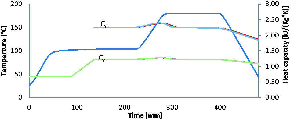
The Figure 23 illustrates the changes in the heat capacity during the process. The resin injection drives a significant change in the value; after adding the resin, the changes that depend on the temperature and the curing reaction are nearly equal in the rubber phase. The cured material is much more sensitive regarding the temperature because uncured material remains in the rubber phase. The density is presented in Figure 24.
Changes in the homogenised density over time.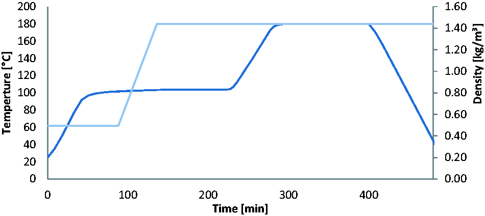
In addition to the thermodynamical results below, the mechanical analysis results are presented. Figure 25 presents the changes in the modulus in the fibre direction for arbitrary points chosen during the process time.
Changes in and range of the modulus in the fibre direction over time.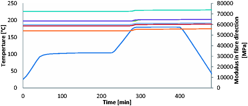
The cured values for the modulus in fibre direction varied from 73900 to 54930 MPa. The influence of the curing and the temperature is smaller in the fibre direction. The most significant influence is based on the fibre volume content. Figure 26 displays the variation in the fibre modulus across the full structure.
Distribution of the modulus in the fibre direction after the curing process.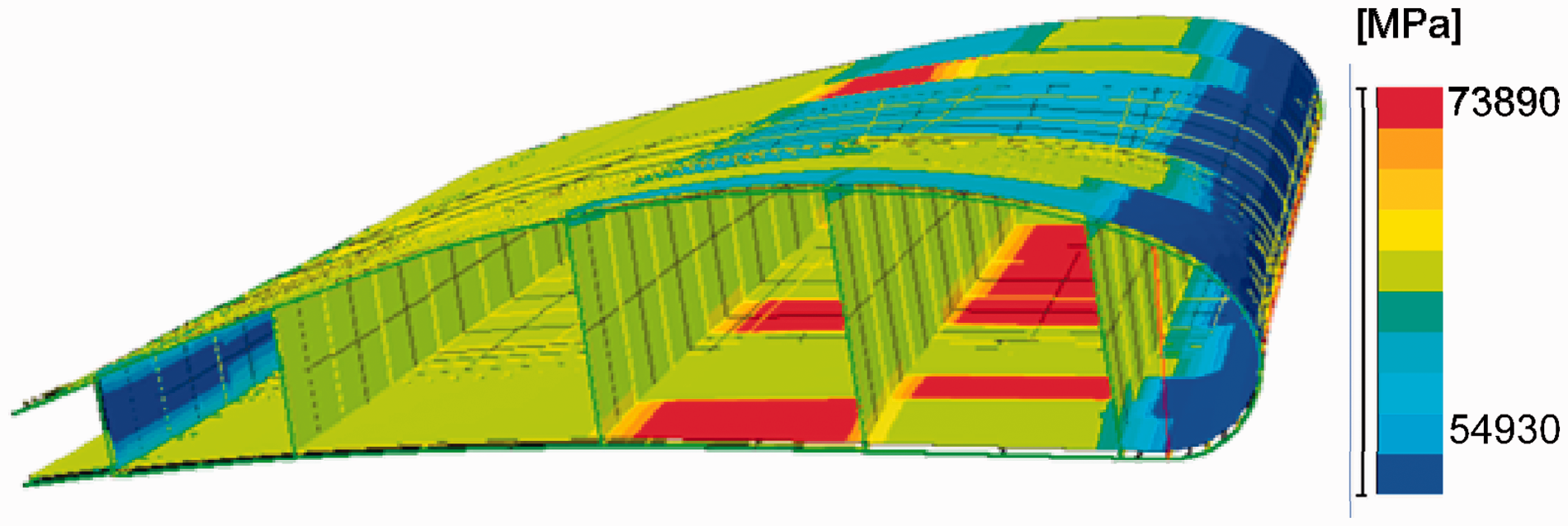
The discrete distribution is an approximation. For more reliable results, continuous mapping methods using experimentally determined data, such as thickness and fibre volume content, would improve the accuracy. Figure 27 presents the changes in the modulus transverse to the ply coordinate system.
Changes in and range of the modulus transverse to the fibre direction over time.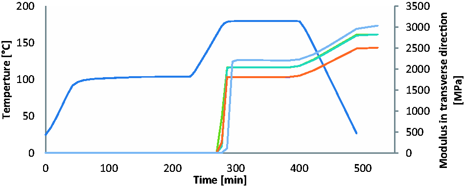
The influence of the resin is dominant in the transverse direction. Accordingly, during the process time, the curing begins in the upper skin. Figure 28 shows the modulus in the transverse direction at 286 min. The values varied from 19 to 7940 MPa.
Modulus in the transverse direction at 286 min (range 7940/19 MPa) and at the end of the process (range 10870/7100 MPa).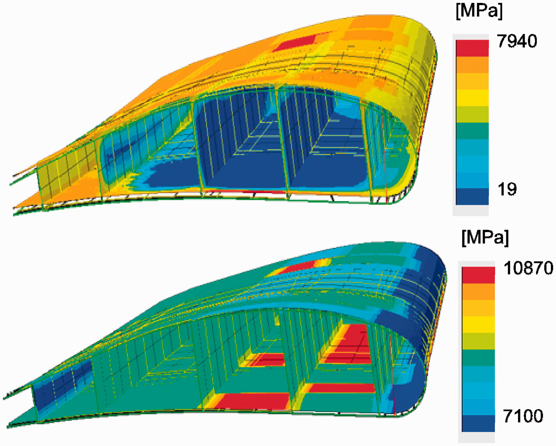
Resulting material properties.
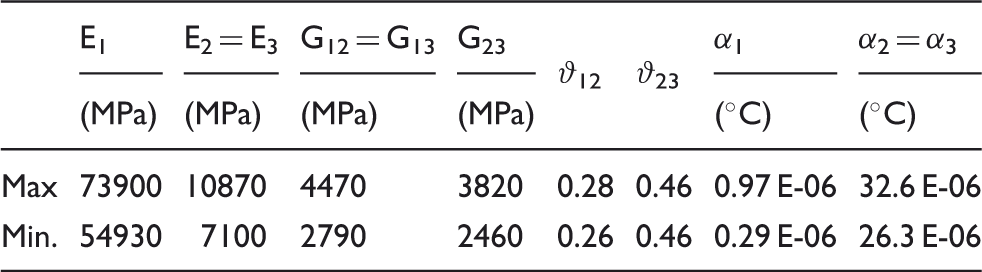
Figure 29 presents the process-induced deformations.
Warpage of the composite part.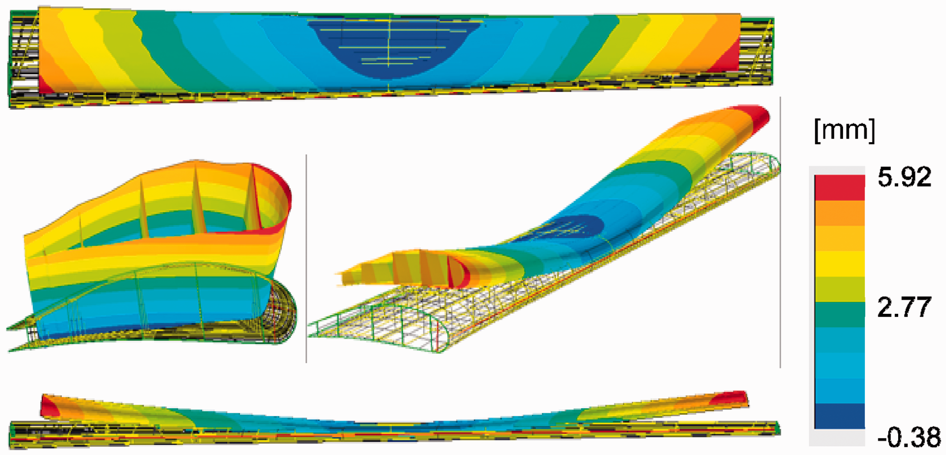
The displacement is displayed as the scalar magnitude projected in out of plane perpendicular to the flap. This representation of the process-induced deformation reveals a displacement from −0.36 mm to 5.92 mm, generating a 6.3 mm total magnitude. In Figure 30, the experimentally measured deformations are shown. The measurements were performed using a structured light 3-D scanner, specifically the Atos system from GOM. The experimental data were analysed using GOM Inspect; this software compares the measurements with CAD references. The problem caused by using measurements is that the same reference coordinates must always be found. For a deformed box structure similar to the given case, matching these coordinates is difficult. Accordingly, there are some methods, such as ‘best fit’, used to align the measured data to the CAD. This method was used in this application because a reference coordinate system was not previously defined. The representation of the deviation values is different from the FE representation. In the FE software, the displacement values are always based on a coordinate system. For the GOM Inspect software, the deviations from the CAD data are calculated normal to the surface. Therefore, the absolute values are not comparable. Figure 30 shows the deviations in the upper and the lower sides.
Measured warpage of the composite part.
The measured warpage from the upper side has a minimum value of −5.71 mm and a maximum value of 2.55 mm, generating a total deformation of 8.26 mm. The lower side deforms from −4.56 mm to 2.40 mm, creating a total deformation of 5.96 mm. This measurement was repeated in the CMF project while using a laser tracking system to evaluate the measurement method. This measurement reached a magnitude of 5.96 mm, highlighting a general problem during warpage analyses for large composite structures. A reliable experimental technique for validating numerical methods, particularly large flexible structures, including thin fuselage skins or panels, is not obvious. The definition of reference coordinate systems, the alignment of experimental data and the possibility of comparing equal values, such as out of plane displacement or deviation in the normal face direction, would mitigate the imprecision. However, the numerical results show the same deformation behaviour (the bent banana shape) and a magnitude of deformation that falls between the GOM measurements and the laser tracking method.
In Figure 31, the material effort is presented over time. To condense the complex stress state, the puck inter fibre effort value was used to reduce the stress tensor to one scalar value. The position of the points are arbitrarily chosen.
Puck inter-fibre effort.
The development of material effort begins after reaching the gel point. This value increases strongly in the rubber phase due to the chemical shrinkage. The material effort caused by chemically induced shrinkage is approximately 15–20%. Afterwards, due to the viscoelastic effect, the effort decreases during the isothermal curing. During the cooling phase, the thermally induced shrinkage increases the material effort, reaching values of 0.85–0.98. Figure 32 presents the effort value distribution across the structure. In regions with high fibre volume content, the stiffness is higher, increasing the effort values.
Puck inter-fibre effort.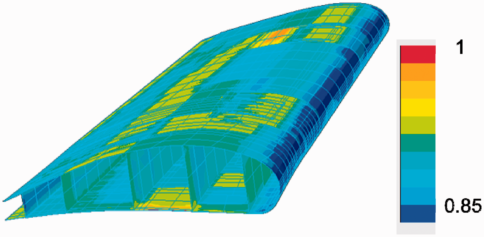
The calculated effort is near the failure index of 1, meaning that inter fibre failure will occur. Figure 33 shows the stress distribution transverse to the fibre direction.
Transverse stress distribution after the process.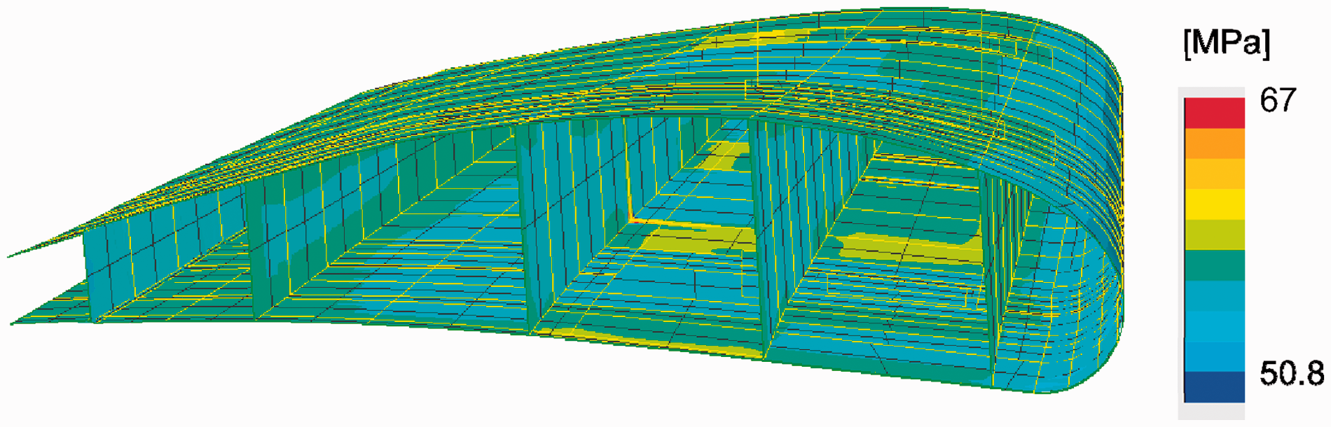
Conclusion
In this study, a sequential thermo-mechanical approach using cure-dependent material model was used to study the cure development and process-induced deformations. A detailed volume model of the mould, component and mandrels was built to analyse the temperature distribution and curing during the entire process. After this thermodynamic analysis, the temperature profiles were transferred to a mechanical analysis as boundary conditions. In this mechanical portion, a multilayer shell discretisation was chosen. The layup of a shell element can be modified without significant pre-processing effort. Therefore, this method can be used to perform sensitivity analyses on the layup, decreasing the computational effort. The simulation method provides the following results during the process time: degree of cure, glass transition temperature, process-induced deformations, residual stress and a complete characterisation of the engineering properties on the ply level. In summary, this simulation method generates accurate values and represents the correct physical behaviour.
Footnotes
Funding
The authors are grateful for the financial support provided by the German Federal Ministry of Economics and Technology (BMWi) within the framework of the national aeronautical research program IV Fact/Vitech (LuFo IV).
Conflict of Interest
None declared.