An anisotropic elasto-plastic material model for injection-molded long fiber-reinforced thermoplastics accounting for local fiber orientation distributions

Abstract

This paper presents an anisotropic elasto-plastic material model for injection-molded long fiber-reinforced thermoplastics. It considers local heterogeneities which are attributed to process-induced variations of fiber orientation distributions and fiber volume fractions. These inhomogeneities have an effect on the mechanical properties and need to be considered in structural computations. In the material model, this is realized through a two-step homogenization procedure. First, an anisotropic stiffness tensor is approximated using mean field homogenization. Second, the plastic behavior is described using Hill’s transversely isotropic yield criterion averaged over the three principal directions of the fiber orientation. The advantage in combining these two approaches is a micro-mechanically based, yet fast numerical calculation of the composite material behavior within an explicit finite element code. The anisotropic material model is calibrated by simulating tensile tests on specimens taken in different directions from an injection-molded plate of fiber reinforced thermoplastic. The spatial variation of fiber orientation distribution and fiber volume fraction throughout the plate is determined from numerical mold filling simulations and is compared with computer tomography scans at different positions. A validation of the model is performed through simulating position-dependent tensile tests on smooth and notched specimens as well as a punch test which is well reproduced.

Keywords

Injection-molded long fiber-reinforced thermoplastic Mori-Tanaka mean field homogenization anisotropic plasticity fiber orientation distribution

Introduction

The great advantages of long fiber-reinforced thermoplastics (LFT) compared to short and infinite fiber-reinforced composites are excellent material properties, e.g. high strength and toughness, in conjunction with processability, e.g. by injection molding. By using low cost ingredients for the matrix such as polypropylene and glass fibers as reinforcements, LFT becomes an efficient material for automotive applications. Especially injection-molded LFT can be used for geometrically complex structures such as airbag housings, frontend-modules or dashboards. A challenging task is to predict the mechanical behavior with respect to its inhomogeneity. Due to the injection molding process, the fiber orientation distribution (FOD) and fiber volume fraction can vary locally and so the mechanical properties. The goal for an applicable use of this material is to simulate the injection molding process and provide information of FOD and fiber volume fraction for structural calculations. An efficient way for calculating effective composite stiffnesses within the consideration of the provided information of the micro structure is to use analytical mean field models. An overview for the application of mean field models for short fiber-reinforced thermoplastics can be found in Tucker and Liang,¹ in which the approach of Mori and Tanaka² is recommended after comparing five different approaches including, e.g., the self-consistent scheme^3,4 and the Halpin-Tsai method.⁵ Furthermore, a validation of mean field models for LFT considering fiber orientation distributions has been carried out by Buck et al.,⁶ resulting in equivalent accuracies for a purely elastic approximation comparing the self-consistent scheme with two variants of the Mori-Tanaka method. All mentioned mean field models are based on the assumption of linear elastic behavior of fibers and matrix. The fibers are assumed to be axisymmetric, identical in shape and size, and can be characterized by the aspect ratio (fiber length divided by fiber diameter). Furthermore, fiber and matrix are assumed to be well bonded at their interface during deformation. Doghri et al.^7–10 or Nguyen et al.^11–13 use mean field homogenization methods, even for nonlinear material behavior. This is done by incrementally linearizing the material behavior. Even some approaches consider fiber/matrix debonding based on an approach of a slightly weakened interface.^12,14,15 A disadvantage of these incrementally formulated micro-mechanical approaches is that they are driving up the CPU times tremendously. Moreover, the determination of the material parameters in this approach is rather laborious.

The aim of the present work is to reduce computational expense and, at the same time, the effort of calibration by combining an analytical micro-mechanical approach for the linear elastic properties with a phenomenological approach for the non-linear plastic properties. The first one is the approach of Mori and Tanaka² which solves the homogenization in one calculation step and therefore it is more effective than, e.g., the self-consistent scheme. The homogenization is used to micro-mechanically approximate a composite stiffness tensor for the linear elastic range. The method, originally suitable for aligned fiber configurations, is extended to account for the local FOD using the approach of Advani and Tucker.¹⁶ The latter is an arithmetical averaging of different orientations of the transversely isotropic stiffness tensor for a unidirectional fiber orientation. The nonlinear plastic behavior is homogenized in a second step through a weighted average over the three principal directions of the FOD. For each direction, Hill’s transversely isotropic yield criterion is used. Furthermore, damage evolution is as well accounted for in a phenomenological manner. Thus, a material model on the use of a two-step homogenization scheme is introduced for structural application for which only a small computing effort is needed. That makes the model applicable for explicit finite element calculation used, e.g., in automotive crash simulations.

Experimental investigations are performed to analyze an injection-molded LFT made of polypropylene and 30 wt% glass fibers. Specimens for tensile and punch tests are taken from different positions of a plate. A spatial heterogeneity is attributed to variations of the local FOD and fiber volume fraction. These data are provided from numerical mold filling simulations and are compared with experimental results. The latter are obtained optically through computer tomography (CT) scans and in addition through density calculations by weighing specimens from different positions to determine local fiber volume fractions.

The material model for LFT has been implemented as a user’s material routine in a commercial finite element code (LS-DYNA). Numerical simulations of various tests are compared with the experimental results.

Notation

Boldface letters in lower case denote vectors, e.g. the position vector $x = x i e i$ , where normal letters with subscripts (i = 1, 2, 3) denote their Cartesian components. Boldface upper case letters denote tensors of second order (e.g. A, $σ, ε$ ), and tensors of fourth order are indicated as $ℂ, A$ and alike. A dyadic product is designated by ⊗. Dots (·) and colons (:) denote contractions over one and two subscripts, respectively. The tensors $I \overset{\land}{=} δ ij$ and $I \overset{\land}{=} 12 (δ ik δ jl + δ il δ jk)$ denote second- and fourth-order symmetric identity tensors, respectively, and δ_ij is the Kronecker delta. The volumetric and deviatoric operators are given by $I vol = 13 I \otimes I$ and $I dev = I - I vol$ , respectively. Therefore, the isotropic elasticity tensor is written as $ℂ = 3 κ I vol + 2 μ I dev$ , where κ is the bulk modulus and μ is the shear modulus.

Approximation of effective stiffness tensor

Mori-Tanaka homogenization

The boundary value problem of an ellipsoidal inclusion embedded in a linear elastic matrix has been solved by Eshelby¹⁷ and is fundamental for the Mori-Tanaka homogenization.² With the concept of the equivalent inclusion problem, the inclusion is considered as a material inhomogeneity. The macro strain $\bar{ε}$ can be defined as

\bar{ε} = c i ε i + (1 - c i) \bar{ε} m

(1)

with the volume fraction of the inclusion cⁱ, the constant strain within the inclusion

ε i

, and the average strain in the matrix

\bar{ε} m

. The strain localization tensor

A

of the dilute distribution is introduced with

ε i = A : \bar{ε}; A = [I + E : ℂ m - 1 : (ℂ i - ℂ m)] - 1

(2)

Here, $ℂ i$ and $ℂ m$ are the isotropic stiffness tensors of the inclusion and the matrix, respectively, and $E$ is the so-called Eshelby’s tensor. Its analytical expression consists of trigonometric functions and depends only on the aspect ratio of the inclusion and the Poisson’s ratio ν^m of the isotropic matrix material. Details can be found, e.g., in the book by Mura.¹⁸ In the approach of Mori and Tanka, the strain localization tensor is not connected to the overall strain but to the average strain in the matrix material

ε i = A : \bar{ε} m

(3)

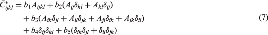
After some algebra, the effective stiffness tensor can be calculated as

ℂ * = [c i ℂ i : A + (1 - c i) ℂ m] : [c i A + (1 - c i) I] - 1

(4)

The embedded inclusion in the matrix is taken to be a prolate ellipsoid approximating a fiber. This leads to a transversely isotropic effective stiffness tensor.

Tensorial description of fiber orientation distribution

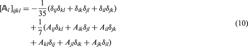
It is often not useful to work with a continuous function to describe the fiber orientation distribution, especially when it comes to the local fiber orientation data mapped from a mold filling simulation. Then, a tensorial form with discrete values is more helpful. Following Advani and Tucker,¹⁶ a tensorial description of a fiber orientation distribution is introduced. In doing so, a unit vector $p (θ, φ)$ is associated with the fiber direction. On the use of spherical coordinates, one can describe every possible fiber orientation on the half of the unit sphere with the variables $(θ, φ) ε [0, π)$ . The integral of the dyadic product of the unit vectors multiplied with the orientation distribution function $Ψ (θ, φ)$ over the surface of the half of the unit sphere yields a tensorial description of the fiber orientation distribution of second and fourth order, respectively

[A] ij = A ij = \oint p i p j Ψ (p) d p

(5)

[A] ijkl = A ijkl = \oint p i p j p k p l Ψ (p) d p

(6)

Orientation averaged effective stiffness

Anisotropic behavior of a material can be described on the use of FOD.¹⁶ The transversely isotropic stiffness tensor $ℂ *$ can be orientation averaged, indicated by $\bar{ℂ} *$ , using the tensors A and $A$ leading to

\bar{C} ijkl * = b 1 A ijkl + b 2 (A ij δ kl + A kl δ ij) + b 3 (A ik δ jl + A il δ jk + A jl δ ik + A jk δ il) + b 4 δ ij δ kl + b 5 (δ ik δ jl + δ il δ jk)

(7)

where the five scalars b_i are related to the five independent components of the transversely isotropic stiffness tensor

C ijkl *

with the 1-axis being the principal direction of anisotropy. It is convenient using Voigt’s notation to write the fourth-order stiffness tensor in a 6 × 6 matrix. With the notation of subscripts

11 \to 1, 22 \to 2, 33 \to 3, 12 \to 4, 23 \to 5

and

13 \to 6

, the five scalars are¹⁶

b 1 = C 11 * + C 22 * - 2 C 12 * - 4 C 44 * b 2 = C 12 * - C 23 * b 3 = C 44 * + 12 (C 23 * - C 22 *) b 4 = C 23 * b 5 = 12 (C 22 * - C 23 *)

(8)

Closure approximation

Often the information of the fiber orientation distribution, especially the data from mold filling simulations, is only available in the form of an orientation tensor of order 2. A closure approximation for the fourth-order tensor $A$ is then needed to use equation (7). The hybrid closure approximation¹⁶ is an efficient way to approximate the missing information for the tensor of higher order. For this, on the one hand, a quadratic form is described as the dyadic product of the tensor of order 2 with

[A q] ijkl = A ij A kl

(9)

This is exact for a unidirectional fiber orientation. On the other hand, a linear form is more accurate for an isotropic fiber orientation distribution and is described by

[A l] ijkl = - 135 (δ ij δ kl + δ ik δ jl + δ il δ jk) + 17 (A ij δ kl + A ik δ jl + A il δ jk + A kl δ ij + A jl δ ik + A jk δ il)

(10)

A rule of mixture is then used to interpolate between both forms with

A hyb = (1 - f) A l + f A q

(11)

and

f = 32 A ij A ji - 12

(12)

The parameter f is a generalization of Herman’s orientation factor. It varies between f = 0 for randomly orientated fibers (isotropic) and f = 1 for perfectly aligned fibers (transversely isotropic). It is to say that the one or the other closure approximation applied separately will lead to poor results for the extreme cases of isotropy or transverse isotropy, respectively. The accuracy has been studied, e.g., in Doghri et al.⁹

Approximation of plastic material behavior

Several publications, e.g. by Doghri et al.^7–10 or by Nguyen et al.,^11–13 consider plasticity in the matrix material and use an incremental homogenization scheme by calculating a tangential stiffness for the matrix material. Implementing these approaches into an explicit finite element code would result in extensive computing times due to the large number of small time steps. The challenging task is an efficient orientation averaging for plastic behavior to achieve feasible CPU time. In contrast to the above-mentioned approaches, the material model developed here is more phenomenological. Plasticity is decoupled from the linear elastic homogenization scheme. For this, Hill’s transversely isotropic yield criterion is used three times in a parallel network (Figure 1) as indicated by the frictional sliding elements. Each unit of the network considers a different direction of anisotropy given by the three principal directions of fiber orientations in terms of the second-order tensor A. Taking the weighted average of the parallel network stress response using the eigenvalues (a₁, a₂, a₃) of the fiber orientation tensor as weights, an orientation averaged elasto-plastic material model is introduced. This simplified orientation averaging for plasticity renders the material model very efficient and improves CPU time tremendously.

Figure 1.

Rheological network of the material model.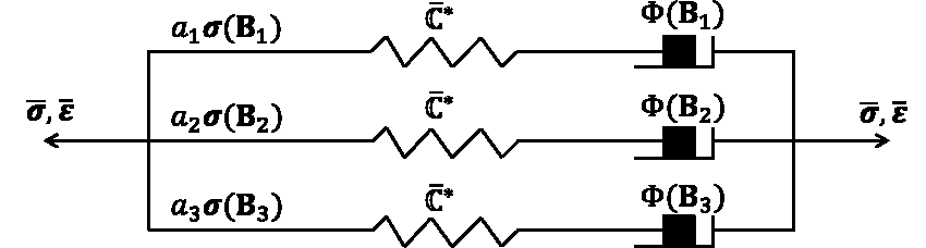

Hill’s yield criterion

The material behaves transversely isotropic for a unidirectional fiber orientation. For this case, the use of Hill’s yield criterion¹⁹ fits perfectly. As the plasticity model needs to account for a particular fiber orientation, an orientation tensor B is introduced, defined solely by the dyadic product

B = e * \otimes e *

(13)

where the unit vector

e *

represents the fiber direction. According to Aravas,²⁰ Hill’s yield criterion can be written on the use of the orientation tensor B in the following form

Φ (σ, B) = (G + 2 F) tr (σ' 2) + 2 (M - G - 2 F) tr (σ' 2 \cdot B) + (5 G + F - 2 M) tr 2 (σ' \cdot B) - σ y 2 (ɛ p)

(14)

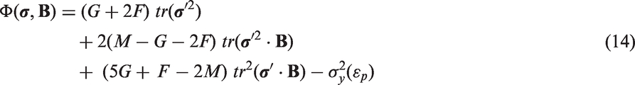
Here, σ_y is the yield stress, $σ'$ is the deviatoric part of $σ$ , and the parameters F, G and M describe the degree of anisotropy. When the parameters are chosen to be F = G = 0.5 and M = 1.5, the criterion reduces to the isotropic von Mises criterion. Hardening depends on the effective plastic strain $ɛ p$ and is approximated with a potential approach

σ y (ɛ p) = σ 0 + h ɛ p q

(15)

where σ₀, h and q are material parameters. The plastic strain rate tensor is obtained from the normality flow rule

\overset{\cdot}{ε} p = \overset{\cdot}{λ} \partial Φ (σ, B) \partial σ

(16)

Orientation averaged plasticity model

To account for arbitrary FOD in the plasticity model, a simplified averaging procedure is suggested here. The principal fiber orientations are given by the eigenvectors $e i *$ of the fiber orientation tensor A as

A = \sum i = 13 \sum j = 13 A ij e i \otimes e j = \sum i = 13 a i e i * \otimes e i *

(17)

where the unit vectors e _i refer to a global coordinate system. The values a_i (

Σ i = 13 a i = 1; a i ε [0, 1]

) are the eigenvalues describing the fiber orientation distribution within the three principal directions

e i *

. Now, three yield criteria

Φ (B i)

are introduced according to the rheological model (Figure 1) using three orientation tensors

B i = e i * \otimes e i *

. This results in three stress tensors

σ (B i)

defined as the numerical solution of

Φ (B i) \leq 0

. An effective stress tensor

\bar{σ}

for the rheological model (Figure 1) is then defined by taking the weighted average using the eigenvalues a_i as weights

\bar{σ} = a 1 σ (B 1) + a 2 σ (B 2) + a 3 σ (B 3)

(18)

The notation $σ (B i)$ symbolizes that each stress tensor depends on the orientation tensor B _i . It has to be emphasized that no orientation averaged yield surface is explicitly formulated in the material model. The parallel network of three independent elasto-plastic material models (Figure 1) is rather averaging the material behavior of three unidirectional fiber orientations according to the FOD. The parameters F, G and M of Hill’s yield criterion are taken equal for the three frictional sliding elements in the network. Details on the implementation and the numerical evaluation of the model are provided in Appendix 1.

Incorporation of damage and failure

When it comes to unloading, irreversible effects have to be separated whether material behavior is referred to damage or plasticity. For an implementation, it is convenient using Voigt’s notation introduced in the Orientation averaged effective stiffness section. In this notation, the second-order symmetric Cauchy stress tensor $σ$ is expressed by a six-dimensional vector $[σ] α (α = 1, \dots, 6)$ . Since interactions between different loading states and damaging effects are not fully understood, six independent damage variables $d α$ are introduced. This leads to a tensorial formulation, where the damage evolution is considered separately for each component of the stress tensor. The damage effect tensor $M$ is then written as follows²¹

M = [1 - d 10000001 - d 20000001 - d 30000001 - d 40000001 - d 50000001 - d 6]

(19)

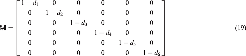
The undamaged stresses $σ α$ are reduced by the term $(1 - d α)$ to calculate stresses of the damaged material $σ α dam$ as

σ α dam = (1 - d α) σ α

(20)

σ dam = M σ

(21)

in direct tensor notation, respectively. For an undamaged state, all six components d_α are equal to 0. If one of the components reaches the value 1, material failure occurs. Damage evolution and failure are taken to depend on the historical maximum of the associated strain

ɛ α, max

. With the material parameters

ɛ f

describing the failure strain and g being the damage evolution exponent, the damage variables are calculated as

d α = (ɛ α, max ɛ f) g

(22)

For convenience, the same failure strain $ɛ f$ and the same damage evolution exponent g are assumed for all strain components. This has turned out to be sufficient when calculating $ɛ f$ and g from tensile tests (Determination of parameters for plasticity and damage section). An extension to an anisotropic failure criterion can be realized easily by introducing different failure strains for the different strain components with respect to the principal fiber directions.²² This would require a more complex test program including also shear in the different directions with repeated loading and unloading.

Experimental investigations

An injection-molded LFT plate of polypropylene with 30 wt% glass fibers (SABIC – STAMAX 30YK270) has been analyzed experimentally. The material was injected through the whole width on the left side of the plate (Figure 2). Specimens for tensile tests were taken from different positions of the plate in angles of 0° and 90° to the flow direction. In addition, computer tomography scans (μCT-scans) have been performed in order to analyze the fiber orientation at three positions indicated in Figure 2.

Figure 2.

LFT plate with 30 wt.% glass fibers manufactured by injection molding (dimensions: 300 mm × 80 mm × 2.8 mm). Specimens (smooth shape) for tensile tests are taken from different positions in 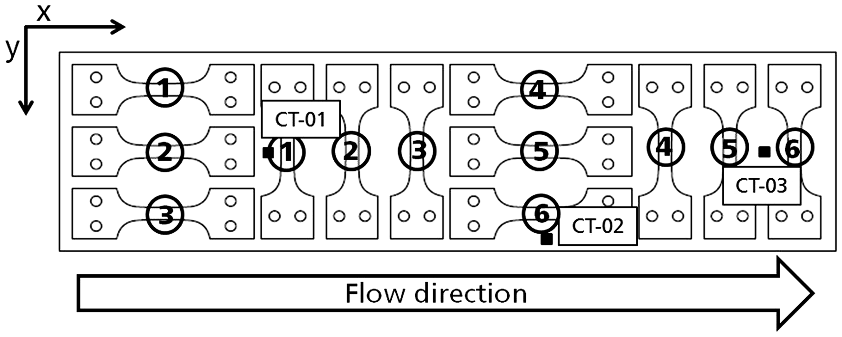$0 \circ$ and $90 \circ$ to flow direction. μ-CT scans are performed at three positions (CT-01, CT-02 and CT-03). Each μ-CT sample has a size of 3 mm × 3 mm × 2.8 mm.

Uniaxial tensile tests

Tensile tests have been performed at a testing speed of 0.01 mm/s at room temperature (23 ± 2℃). The parallel region in each specimen is (14 mm × 5 mm). Elongation has been measured over a length of 10 mm within the parallel region using an extensometer. The force was determined directly at the standard Instron Universal Testing machine using a load cell. The results in terms of stress strain curves are shown in Figures 3 and 4. The engineering strain is determined from the elongation divided by the gauge length of 10 mm and the engineering stress results from the measured force divided by the initial cross section of (5 mm × 2.8 mm). In analyzing strength and stiffness values for the various positions, differences can be clearly identified. According to the symmetry of the plate, tensile tests for positions 1 and 3 performed in 0° to the flow direction show the same response in terms of the stress–strain curves being stiffer than that for position 2 (Figure 3). The same trend can be observed by comparing positions 6 and 4 with position 5. Moreover, strength and stiffness increase with the flow path, i.e. a generally softer response is observed close to the gate.

Figure 3.

Tensile tests in 0° to the flow direction.

Figure 4.

Tensile tests in 90° to the flow direction.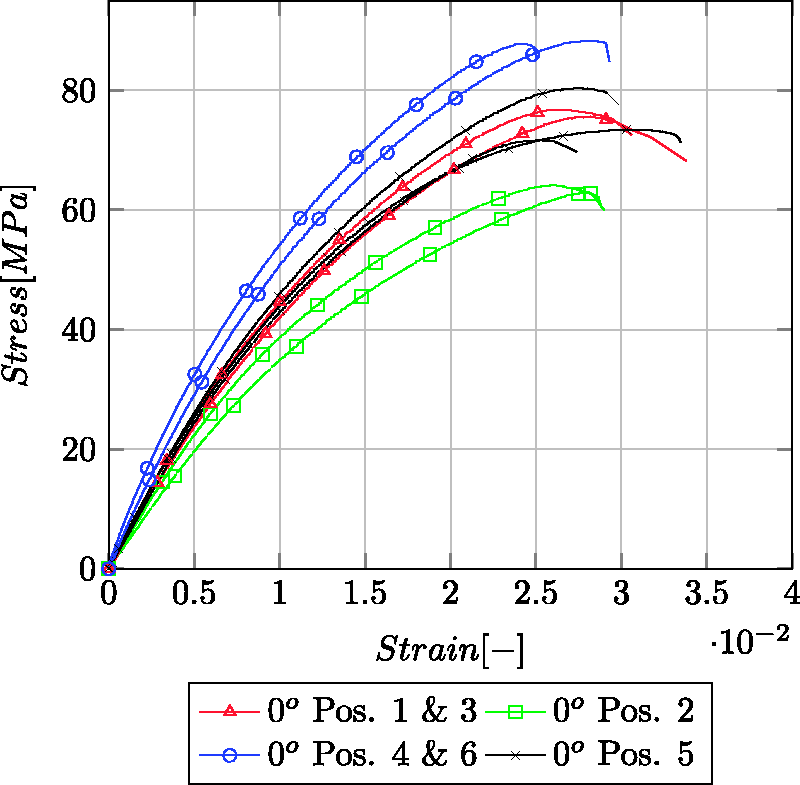

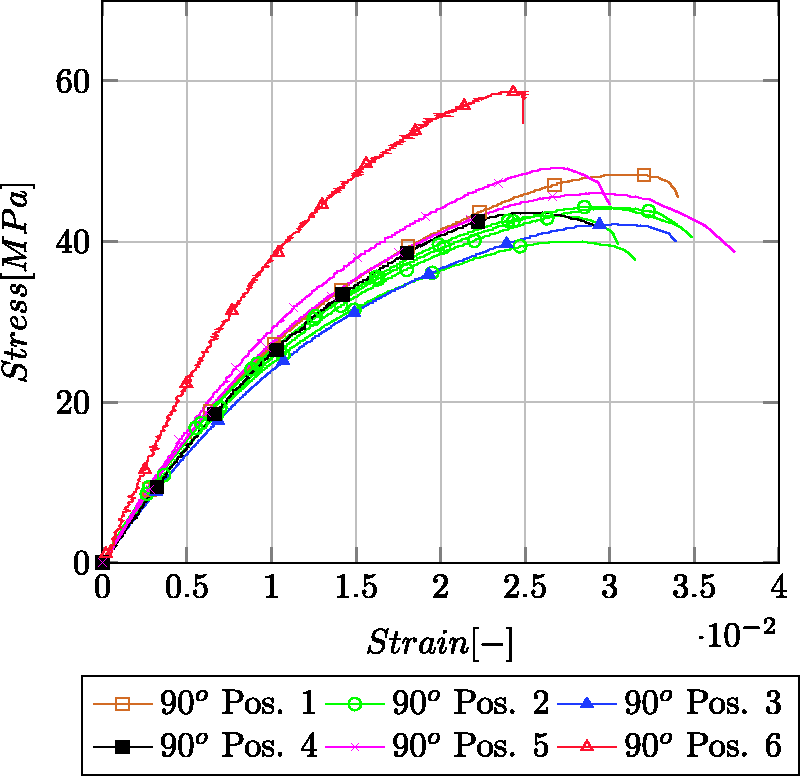
This effect is much less pronounced in tests on 90°-specimens (Figure 4). A clear edge effect is observed at position 6 with the result of an extraordinary high strength and stiffness compared to the other positions. An explanation of these findings is provided in the following subsection based on the measured fiber orientations.

Analysis of fiber orientation distribution

A typical fiber orientation distribution through the thickness of the plate is shown in Figure 5 where a polished cross section from the center region of the plate is analyzed with a light microscope. The characteristic flow induced layered structure of fiber orientation can be observed. Most of the fibers lie in flow direction and can be identified by long ellipsoidal shapes. A thin layer of fibers orientated perpendicular to the flow direction exists in the core region identified by circular shapes. This crossing fiber orientation is typical for injection molded LFT.

Figure 5.

Polished cross section from the center region of the plate under a light microscope showing fibers aligned to the flow direction (ellipsoidal shapes) and perpendicular to the flow direction (circular shapes).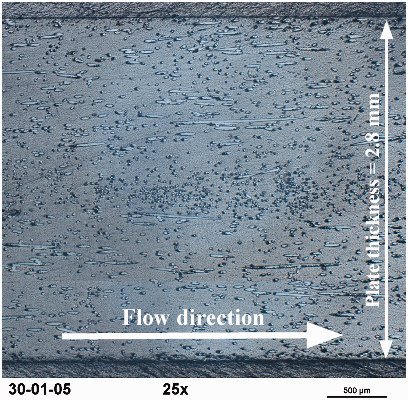

According to Figure 2, CT-scans are performed for milled cubes over the complete thickness of the plate from three different positions. A micro computer tomograph with a 225 kV X-ray tube has been used and scans are performed with a voxel size of 2.7 µm. The data were analyzed using the software tool MAVI (Modular Algorithms for Volume Images).²³ The software is able to analyze a fiber orientation distribution through a 3D image. Each cube-shaped specimen is divided into 18 layers over the thickness and FOD is represented by a second-order tensor. In MAVI, a Hessian matrix is built from the directional differences of the gray scale from pixel to pixel. An eigenvalue analysis of the Hessian matrix is performed for each pixel classified as the gray value of the fiber material. The eigenvector v belonging to the smallest eigenvalue describes the direction of the smallest change of the gray value and therefore the most likely fiber direction. The fiber orientation tensor of second-order $[A] ij$ is then calculated through the dyadic product represented by

A = v \otimes v

(23)

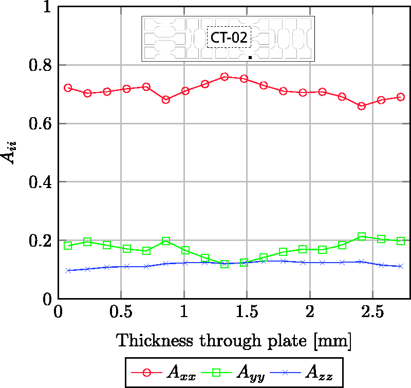
For each of the 18 layers, the arithmetic mean is calculated on the use of all fiber orientation tensors belonging to all pixels in that considered region. In Figures 6 to 8, the diagonal components of the orientation tensors are plotted for each CT scan over the thickness. The coordinate system is according to Figure 2, i.e. the x-coordinate is along the flow direction and the z-coordinate points in thickness direction of the plate. In Figures 6 and 8, the already mentioned typical crossing of fiber orientation can be observed. A clear edge effect can be analyzed in Figure 7 with most of the fibers directed in flow direction A_xx.

Figure 6.

Fiber orientation tensor from CT scan at Position CT-01.

Figure 7.

Fiber orientation tensor from CT scan at Position CT-02.

Figure 8.

Fiber orientation tensor from CT scan at Position CT-03.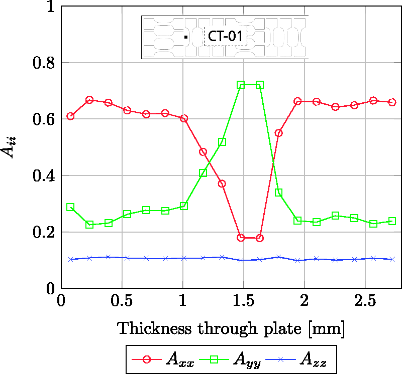

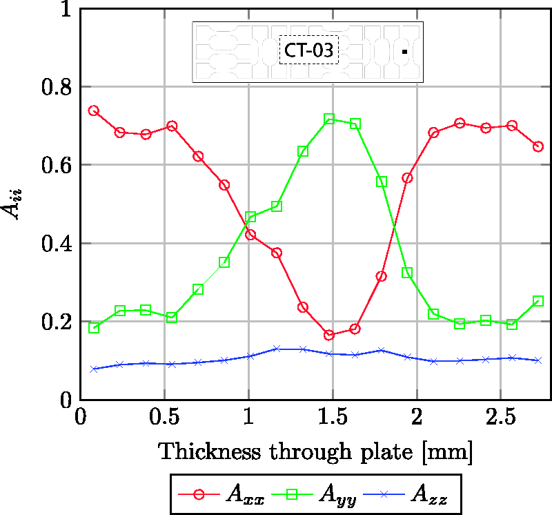
The fiber orientation distribution analysis based on the use of a voxel mesh created trough a CT-scan has to be taken with some care. The amount of fibers in plate thickness direction is likely to be overestimated. The reason is that a bunch of fibers with an in-plane direction often creates a voxel field of glass material without interruption in thickness direction and will be identified as a fiber with an out-of-plane direction. As a consequence, the value A_zz will be overestimated which leads to an underestimation of A_xx and A_yy.

Analysis of fiber diameter

The weight-averaged fiber length of this material is known from suppliers analysis and is about 2.4 mm for plate-shaped structures. The fiber radius has been analyzed in polished cross sections using a light optical microscope (Figure 9). The radii between 6 µm and 12 µm have been observed. Thus, the aspect ratio can vary between approximately 100 and 200. The unprocessed fiber length is approximately 10 mm. It can be assumed that the plate contains some amount of unbroken fibers. This means that the aspect ratio can be much higher for certain fibers than the average. The effect of the fiber length on the mechanical behavior and the response of the material model are discussed in the Material model calibration and validation section.

Figure 9.

Polished cross section under a light microscope showing the variation of the fiber radius between 7.62 µm and 11.36 µm.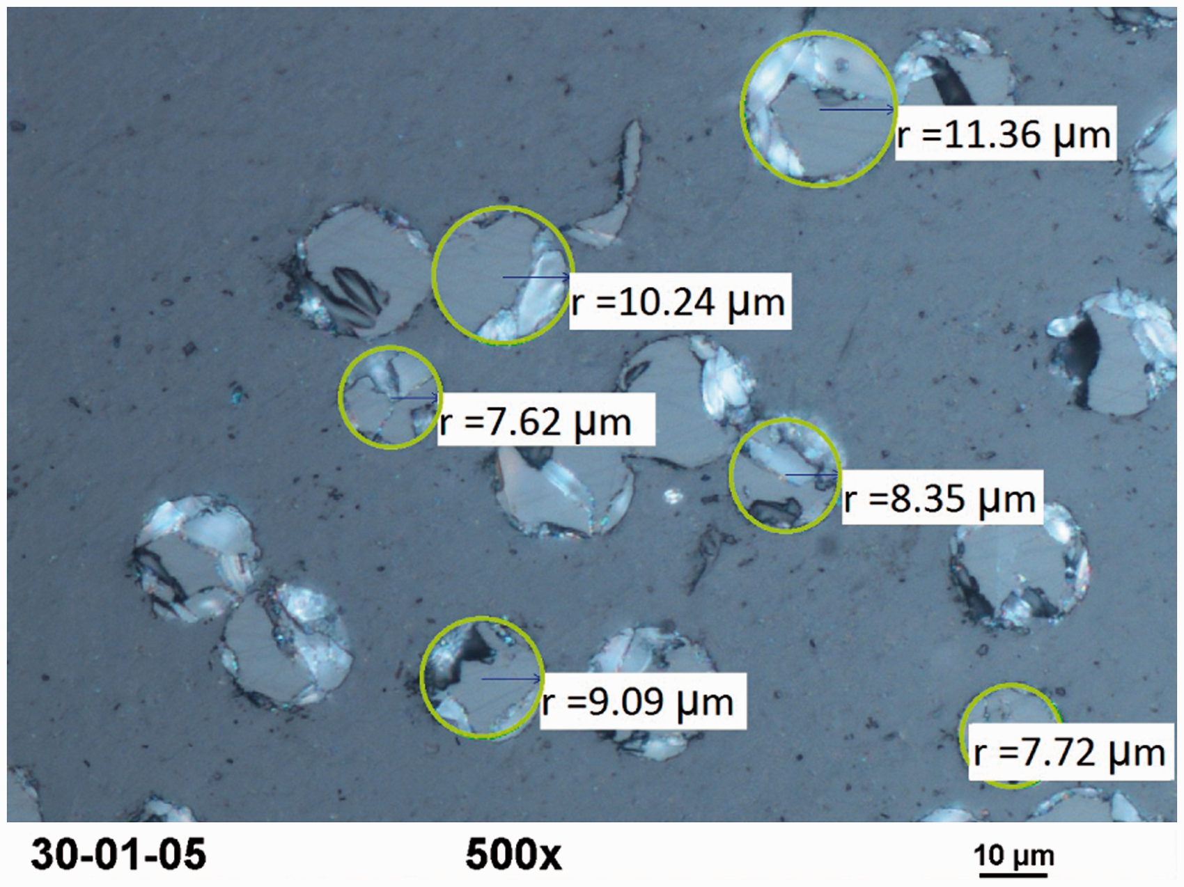

Analysis of fiber volume fraction

The fiber volume fraction has been analyzed by two independent ways. To determine the mass density ρ_total, the tensile specimens have been weighed. This was done for each specimen. A fiber volume fraction c_f is then calculated with

c f = (ρ total - ρ pp) (ρ glass - ρ pp)

(24)

where

ρ pp = 905 kg / m 3

is the mass density of polypropylene and

ρ glass = 2600 kg / m 3

is the mass density of glass. Both values are given from the material supplier.

Additionally, the fiber volume fraction is analyzed from 3D images of a CT-scan using MAVI Software.²³ The fiber radius must be given for calculation and therefore the solution of the fiber volume fraction may have faults. It is recalled that the radii vary between 6 µm and 12 µm. A detailed information about the algorithm of MAVI can be found in the user’s manual.²³ In Figure 10, both results for the fiber volume fraction c_f along the x-coordinate of the plate are shown. The results from the CT-scans are averaged over the whole thickness of the plate. Figure 10 shows that according to both methods, the fiber volume fraction increases with the flow path. This corresponds to the results of Figures 3 and 4 where strength and stiffness increase in the same way.

Figure 10.

Fiber volume fraction from method of weighing and CT analysis.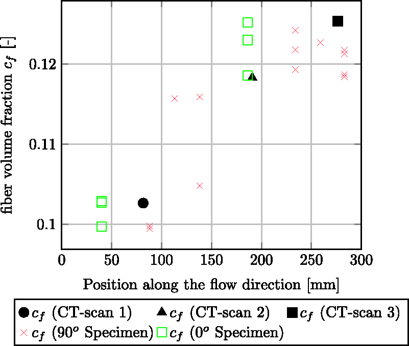

Fiber orientation distribution and volume fraction from mold filling simulation

The process of injection molding has been simulated using the software CoRheos (Complex Rheology Solver) developed at Fraunhofer Institute for Industrial Mathematics ITWM. A coupling between fluid–fiber and fiber–fiber interaction has been considered for a good prediction of fiber orientation distribution throughout the plate. In addition, the influence of fiber volume fraction coupled with the fiber orientation is taken into account. The numerical model of the plate is discretized with nine finite volume cells through the thickness, 80 cells in width and 200 cells in length direction. Further details about the implementation of the rheological solver can be found in recent publications.^24–26

For validating the accuracy of the numerically predicted fiber orientation distribution, simulated results are compared with the CT-scans. For the three positions CT-01, CT-02 and CT-03 (see Figure 2), results are compared and shown in Figures 11 to 13. It can be clearly seen that the simulated values of A_zz are generally lower than in the experiments. Thus, simulated values of A_xx and A_yy are higher than the experimental results. For reasons mentioned in the Analysis of fiber orientation distribution section, the fiber orientation in thickness direction is somewhat overestimated in the CT analysis. In view of this, the simulated results are in reasonable agreement with the experiments.

Figure 11.

Fiber orientation tensor from CT scan and mold-filling simulation at position CT-01.

Figure 12.

Fiber orientation tensor from CT scan and mold-filling simulation at position CT-02.

Figure 13.

Fiber orientation tensor from CT scan and mold filling simulation at position CT-03.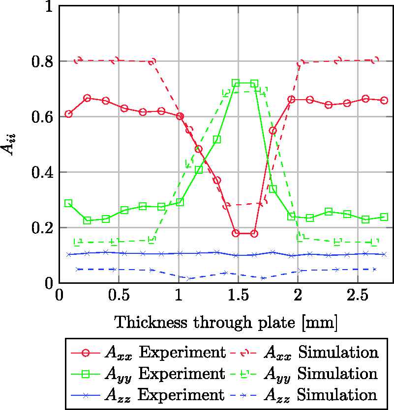

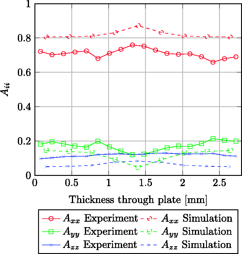
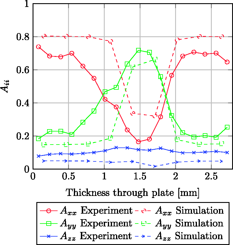
Figure 14 shows the comparison between the fiber volume fractions at the three positions of the CT-scans and the numerically determined fiber volume fractions from the mold filling simulation. The simulated data are in a good agreement with the experimental results showing the increase of the fiber volume fraction with the flow path. The latter has been analyzed in Figure 10.

Figure 14.

Fiber volume fraction from CT analysis and mold-filling simulation.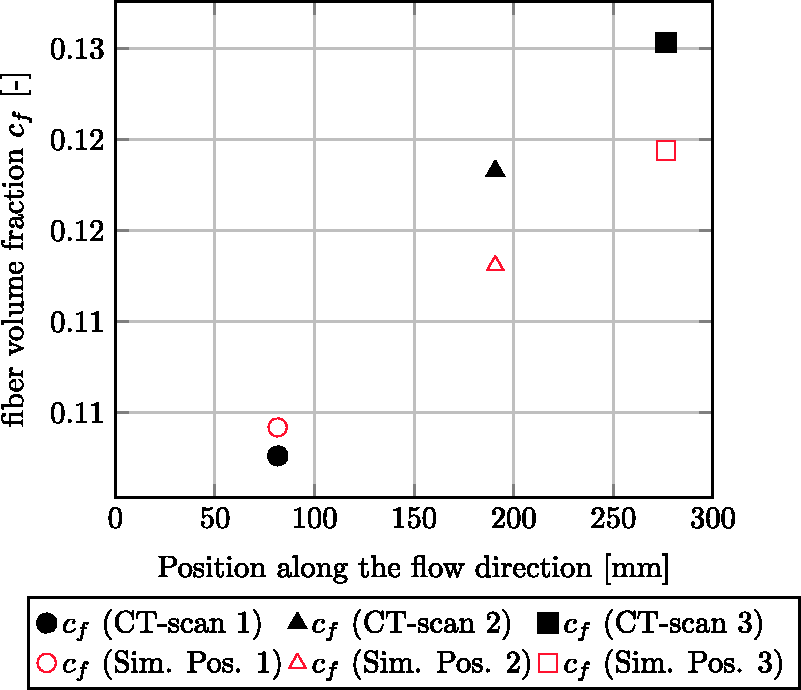

Material model calibration and validation

The geometry of the tensile test specimen (smooth shape) used in the experimental investigations of the Experimental investigations section has been discretized with 3288 eight-noded finite elements of hexahedral shape (Figure 15) with one point reduced integration. In the center region of the size (14 × 5 × 2.8 mm), the uniform element edge size measures 0.5 mm. The engineering strain in the simulations of the tensile tests has been determined (analogous to the experiments) from relative nodal displacements divided by their gauge length of 10 mm. The boundary conditions are applied to the nodes at the surfaces on the left and right side of the specimen as displayed in Figure 15. According to the corresponding coordinate system, the displacements in $y'$ -direction are fixed at the nodes on the left side and a prescribed velocity $V 0 = 1 m / s$ is applied at the nodes on the right side. For both sides, the displacements in $z'$ -direction are fixed and traction free boundary conditions are applied in $x'$ -direction.

Figure 15.

Finite element model of tensile test specimen (smooth shape) showing element size and boundary conditions.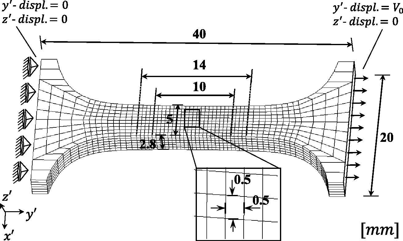

Validation of anisotropic stiffness tensor

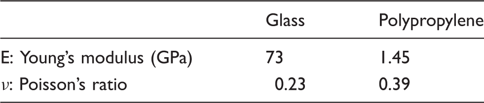
For the approximation of the anisotropic stiffness tensor, the material properties of the components are taken from suppliers informations listed in Table 1. Young’s modulus and Poission ratio of polypropylene have been determined through tensile tests at room temperature according to DIN-EN-ISO-527. Similar values are given in the literature.^12,27

Table 1.

Elastic parameters of isotropic base materials.

	Glass	Polypropylene
E: Young’s modulus (GPa)	73	1.45
ν: Poisson’s ratio	0.23	0.39

In the first homogenization step using the Mori-Tanaka approximation according to the Mori-Tanaka homogenization section, the transversely isotropic stiffness tensor requires the information of the fiber aspect ratio. As mentioned in the Analysis of fiber orientation distribution section, this aspect ratio can vary due to process-induced fiber breakage with different lengths and fiber diameters. Theoretical predictions of the anisotropic Young’s moduli are shown in Figure 16 over a variation of the aspect ratio. It can be seen that an aspect ratio larger than 80 does not have much influence on the approximated stiffness. Fiber length of 2.7 mm and fiber diameter of 0.017 mm are mean values. This gives an aspect ratio of 158 (dashed line in Figure 16) with a Young’s modulus of about 10.72 GPa in fiber direction.

Figure 16.

Anisotropic Young’s moduli of transversely isotropic stiffness tensor. Influence of fiber length in Mori-Tanaka approximation.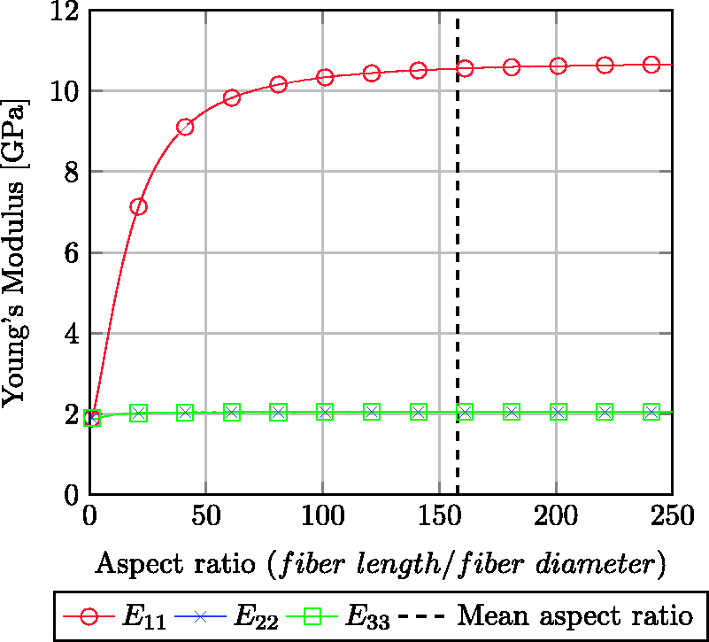

Taking into account the FOD for approximating the stiffness tensor according to the Orientation averaged effective stiffness section, the FOD from the injection molding simulation and the CT-data can be used in linear elastic finite element simulations of the tensile tests. Therefore, results for FOD and fiber volume fraction accounting for variations over the thickness have been mapped to the finite element model of the tensile test specimen. A comparison of the linear elastic calculations using the numerical model of Figure 15 with FOD from μCT-scan and FOD from mold filling simulation is shown in Figure 17 along with the experimentally obtained stress–strain response. It can be seen that the simulated FOD-data give a stronger anisotropy with a higher stiffness in flow direction and a lower stiffness perpendicular to the flow direction than the FOD from the μCT-scan. Simulated results are compared with experimental tests on specimens close to the position of CT-01. In the range of experimental scatter, both FODs lead to reasonable simulation results in the linear elastic regime.

Figure 17.

Linear elastic FEM calculations of tensile tests using FOD from CT-scan CT-01 (dashed lines) and FOD from mold-filling simulation at the same position (solid lines). Comparison with experimental data from close positions (black dotted lines).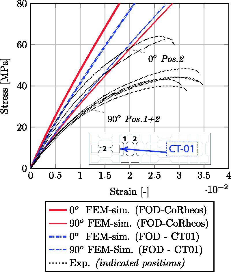

Determination of parameters for plasticity and damage

For applications of the material model such as automotive crash simulation, the requirements are basically a good prediction of the elasto-plastic behavior and the onset of failure under monotonic loading. In the following, damage affects are first neglected and only plasticity parameters of the model are fitted to the experimental tensile tests. The results are shown in Figure 18 where the FOD obtained from mold filling simulation (CoRheos) has been used. It has to be mentioned that a slightly higher Young’s modulus for polypropylene (than given by supplier, Table 1) of $E PP = 1.8 GPa$ has been adopted here which leads to better results. This correction appears justified because there is no information on material parameters of polypropylene inside the composite and it is very likely that the elastic parameters of the base material differ from those inside the composite. For example, material behavior could be influenced by the degree of crystallization affected by the presence of fibers in the composite. For a separation of plasticity and damage, uniaxial tensile tests with unloading have been performed. As can be seen in Figure 19, by neglecting damage the elasto-plastic model yields a significantly stiffer unloading response than the experimental data. Therefore, damage according to the Incorporation of damage and failure section is included in the model, and the improved model performance with re-adjusted plasticity parameters is shown in Figure 20. It is noteworthy that the damage formulation (22) with equal values of the parameters for all components gives good results in predicting the anisotropic material behavior.

Figure 18.

Tensile tests: Experimental results (dotted lines) and FEM simulations using elasto-plastic model without damage (solid lines). Parameters: $E PP = 1.8 GPa, ν PP = 0.39,$ $E Glass = 73 GPa, ν Glass = 0.23, σ y = 15 MPa,$ $h = 480 MPa, q = 0.43, F = 3.0, G = 0.5, M = 1.5$ .

Figure 19.

Loading–unloading tensile tests: Experimental results (dotted lines) and FEM simulations using elasto-plastic model without damage (solid lines).

Figure 20.

Loading–unloading tensile tests: Experimental results (dotted lines) and FEM simulations using elasto-plastic model with damage (solid lines). Parameters: $E PP = 1.8 GPa, ν PP = 0.39,$ $E Glass = 73 GPa, ν Glass = 0.23, σ y = 10 MPa,$ $h = 470 MPa, q = 0.27, F = 3.0, G = 0.5, M = 1.5,$ $g = 1, ɛ f = 0.076$ .

Validation of position dependence

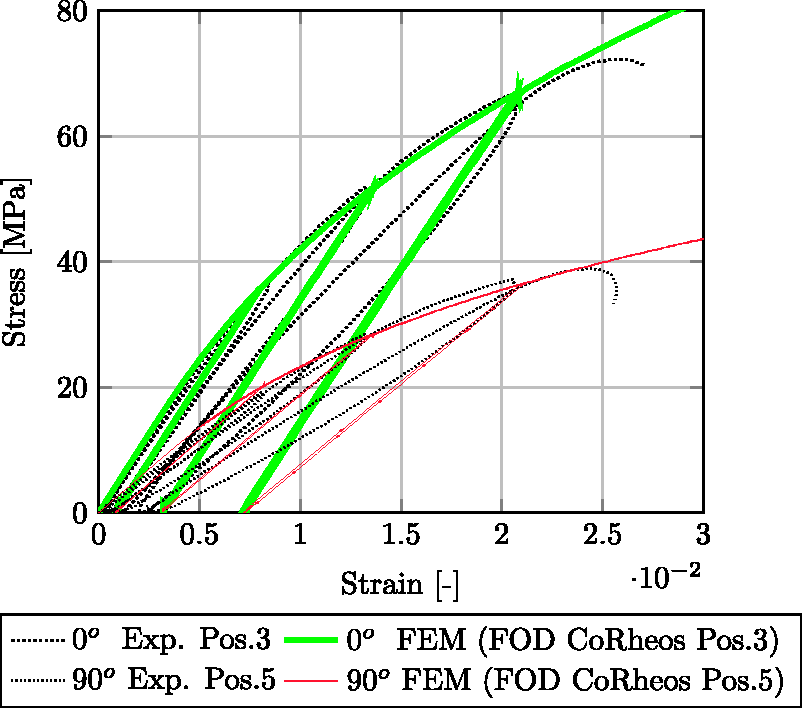
Tensile test specimens corresponding to different positions in the plate (Figure 2) are now simulated using calibrated material parameters according to Figure 20. Each tensile test specimen is allocated to a position on the plate and the fiber orientation distribution from the mold filling simulation is mapped onto the FEM model, by also taking into account the variation of the FOD through thickness according to Figures 11 to 13. Results for all specimens in 0° to flow direction are shown in Figure 21. The proper tendency with the highest strength and stiffness at positions 4 and 6 and the softest response at position 2 is reproduced well. Due to symmetry, the simulated tensile test of position 1 has no particular difference to the simulation of position 3. The same holds for comparing positions 4 and 6.

Figure 21.

Tensile tests in 0° to the flow direction: comparison between FEM simulations with damage and failure (solid lines) and experiments (dotted lines).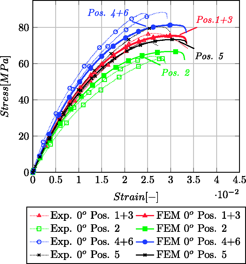

As mentioned in the Uniaxial tensile tests section, no clear position dependency for 90° tensile tests of positions 1 to 5 has been observed. The simulations show comparable results (Figure 22). The edge effect of position 6 with high strength and stiffness is not represented correctly due to low correspondence of the FOD in the mold filling simulation at this edge influenced region.

Figure 22.

Tensile tests in 90° to the flow direction: Comparison between FEM simulations with damage and failure (solid lines) and experiments (dotted lines).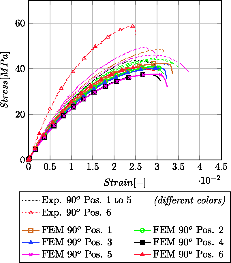

Simulation of tensile tests with notched specimens

For further validations of the introduced material model, investigations have been made to analyze the material under different loading conditions. Therefore, two additional types of specimens have been cut out from the injection-molded plate. As shown in Figure 23, notched tensile test specimens (marked in black) are taken from various positions of the plate in two directions. Additionally, round specimens for punch tests (marked in gray) have been extracted.

Figure 23.

LFT plate with specimens for notched tensile tests taken from different positions in 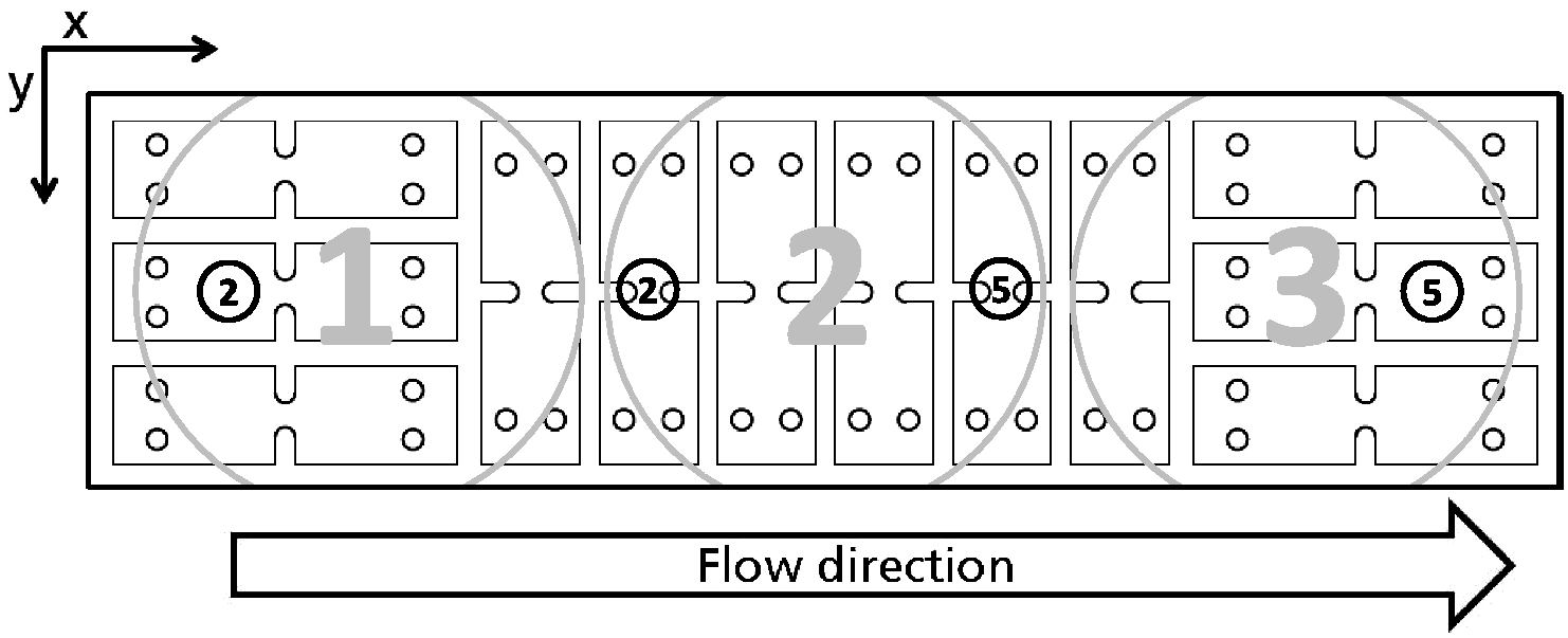$0 \circ and 90 \circ$ to flow direction (marked in black). Specimens for punch tests taken from three positions (marked in gray).

The tensile tests on notched specimens with notch radii of 2 mm and a ligament of 5 mm have been analyzed at four different positions, two positions in 0° and two positions in 90° to the flow direction. The smallest cross section A₀ measures (5 mm × 2.8 mm). The experimental conditions are according to the Uniaxial tensile tests section. The force is normalized over the smallest cross section through ( $F / A 0$ ). Elongation (Δl) has been measured over a length of 10 mm, hence ± 5 mm from the center of the specimen, using an extensometer.

The geometry of the notched tensile test specimen has been discretized with 4344 eight-noded finite elements of hexahedral shape (Figure 24). Element size in the region of localized deformation as well as element type and boundary conditions is the same as for the smooth tensile tests. The simulated elongation is determined as relative nodal displacements at a distance of 10 mm.

Figure 24.

Finite element model of notched tensile test specimen showing element size and boundary conditions.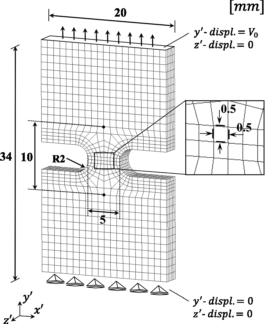

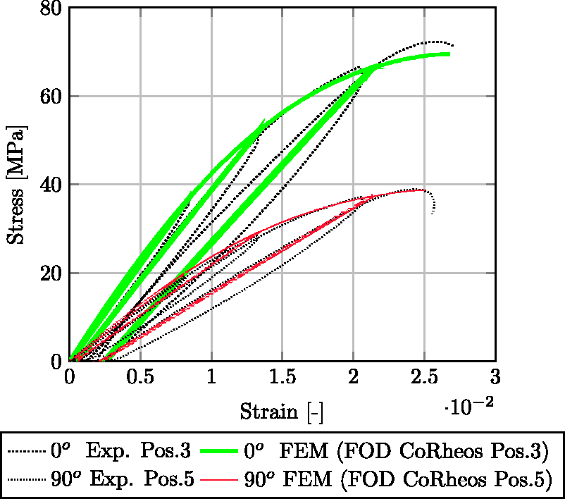
The results of the experimental tests and numerical calculations are shown in Figure 25. No further calibrations on the material model have been made, and hence all parameters of the model correspond to those determined in the Determination of parameters for plasticity and damage section. Similar to the examination of the smooth tensile tests (Experimental investigations section), the experimental results of the notched specimens (Figure 25) show a clear position dependency for the 0° direction. The numerical results in Figure 25 show a better agreement for position 5 than for position 2 which is slightly overestimated by the simulation. As the position dependency in 90° between positions 2 and 5 is hardly recognizable, only the FOD of position 2 is mapped to the numerical model. Calculated results are in reasonable agreement with the experiments. The end point of the curves corresponds to the ultimate failure of the specimens. Failure occurs in a rather brittle manner in the simulations while it appears to be more ductile in the experiments.

Figure 25.

Tensile tests on notched specimens: Comparison between FEM simulations with damage and failure (solid lines) and experiments (dotted lines).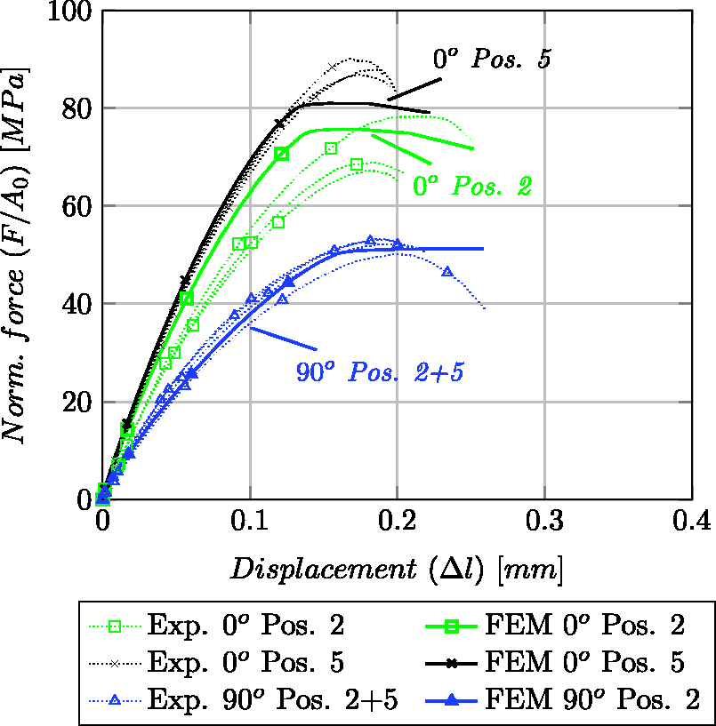

Simulation of punch tests

Punch tests have been performed on round specimens of 90 mm diameter taken from three different positions of the plate (Figure 23). For the experimental setup and the numerical model (Figure 26), the specimen is fixed between two metal plates with round openings. The bottom fixation measures an opening diameter of 33 mm. The top fixation has an opening diameter of 27 mm with a smooth edge of radius 0.5 mm. The specimen did not slip between the two fixations. The round indenter of radius 10 mm pushes through the openings with a constant velocity of 0.01 mm/s while deforming the specimen. The force and the displacement have been determined directly at the standard Instron Universal Testing machine.

Figure 26.

Finite element model of punch test.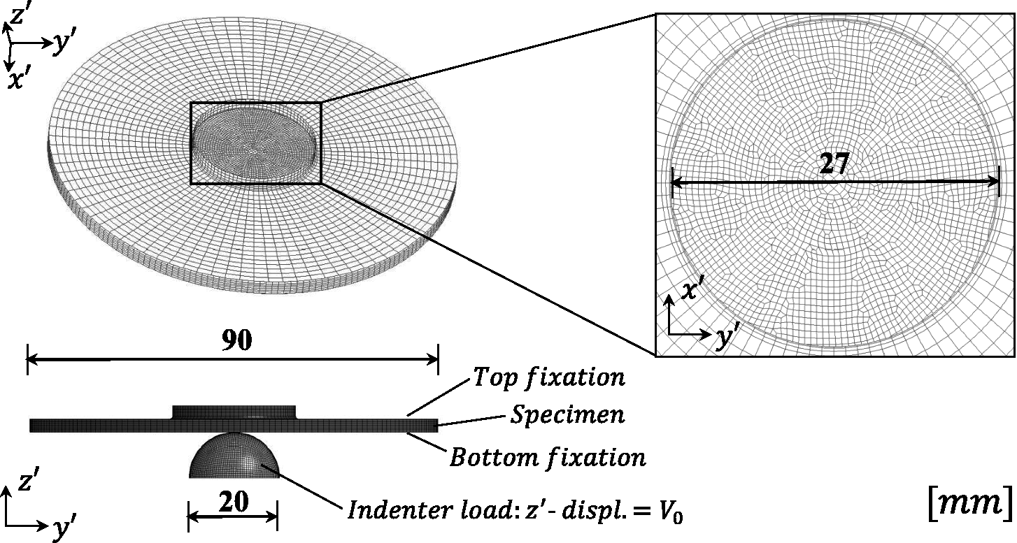

As shown in Figure 26, the numerical model of the specimen is meshed with 59010 eight-noded solid elements on the use of automatic mesh generation (HyperMesh, Altair Computing Inc., Troy, Michigan, USA). An element size of 0.5 mm is realized in the core region with six elements through thickness. Plates for fixation and indenter are modeled as rigid bodies. For contact definition, a penalty contact type is used. A high friction coefficient of 0.99 is defined to clamp the specimen between the two rigid plates and a low friction coefficient of 0.1 is considered for the contact between the indenter and the specimen. All parameters of the material model correspond to the ones determined in the Determination of parameters for plasticity and damage section.

A comparison between experimental results and numerical solution of the force–displacement curves measured at the indenter is shown in Figure 27. In contrast to the smooth and notched tensile tests, no significant position dependence is seen in the punch tests (dotted and dashed curves). Consequently, only one position (position 2) is simulated. The calculation is in good agreement with the experimental results by comparing the slope and the maximum force. Due to an early and very fine scale crack initiation observed in the experiments, the slope gets successively flatter. In the simulation result, in contrast, the force drop after the maximum is overestimated and more sudden due to the coarse element size (0.5 mm) which is not fine enough to resolve the fine scale crack propagation.

Figure 27.

Punch test: Comparison between FEM simulation with damage and failure (red solid line) and experiments (dotted and dashed lines).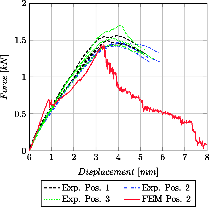

The differences between experiments and simulation can be better understood by the visual observation of the fracture pattern (Figure 28). In the numerical model (left picture), crack propagation is influenced by element size and orientation. After the first element reaches the failure criterion and gets deleted, the neighboring elements are strongly affected by the large imperfection. The experimental observation in contrast shows a stable crack propagation whereas finely branched cracks join to coarse cracks. However, the fracture pattern just after the maximum force shown in Figure 28 is in good agreement.

Figure 28.

Comparison of fracture pattern in the punch test between numerical calculation (left) and experiment (right) just after maximum force.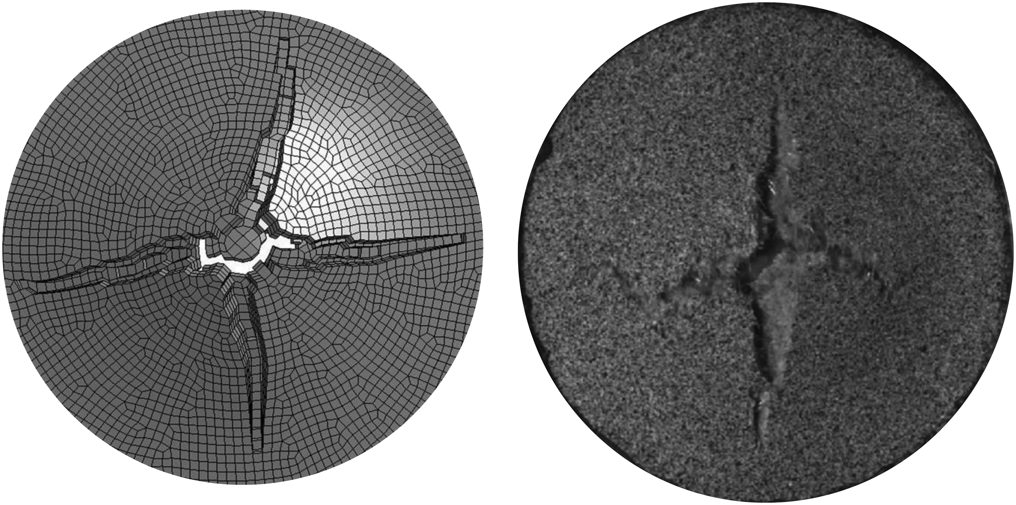

It has to be emphasized in summary that the simulation of the complex punch test matches well, in terms of maximum force, initial slope (Figure 27) and fracture pattern (Figure 28) which are usually not as well reproduced in numerical simulations.

Summary and conclusions

Using a two-step homogenization scheme, an anisotropic elasto-plastic material model for LFT has been developed. It has been shown that the micro-mechanical approach of Mori and Tanaka with the orientation averaging according to Advani and Tucker performs well for the approximation of the anisotropic stiffness tensor. The second homogenization step accounting for the plastic material behavior is an orientation averaging over the three principal fiber directions and a rather rough estimate, but obviously precise enough for the present application. Damage and failure have been considered within a rather simple approach and proved to be sufficient in the performed simulations. This is due to the fact that failure strains in 0° and 90° to the flow direction do not show significant differences. This might not be the case for stronger anisotropy (e.g. aligned fiber orientation) where anisotropic damage and failure criteria should be used. Experiments and simulations with complex loading situations have been performed on notched specimens and a punch test showing satisfying results. The complex crack initiation and crack propagation observed in the experiments of the punch test will only be able to be reproduced with a small finite element mesh size. As this was not the goal here, we have only considered an element size of ca. 0.5 mm edge length. An improved model should consider also damage evolution depending on the load case, e.g. stress triaxiality, and element size. A fiber length distribution has not been considered in the proposed model. As shown in the Validation of anisotropic stiffness tensor section, a variation of the fiber length would not have a strong effect on stiffness calculation because the fiber length of the examined material is in the range of saturation. Hence, this material mostly contains fibers with a fiber length close to the critical fiber length for which a maximum stiffness is achieved according to the Mori-Tanaka model. It might be reasonable to assume that the fiber length plays a different role in case of damage and failure regarding experimental observations.²⁸ This effect is not yet studied well enough and therefore not considered in this approach. The present results indicate that the approach suggested here can be successfully employed to predict nonlinear anisotropic material behavior of injection-molded long fiber-reinforced composites in an explicit finite element calculation. Experimental investigations on different FODs need to be done for further refined validations. Other stress states, e.g. shear loading, should also be taken into account for a detailed analysis of the proposed model. The extension of the model considering a strain rate dependency is subject of future work.

Footnotes

Acknowledgments

We would like to thank for the rheological simulations with CoRheos and the computer tomography analyses of the material studied in this work. The support by our colleagues from Fraunhofer ITWM in Kaiserslautern, Germany, is gratefully acknowledged.

Declaration of Conflicting Interests

The author(s) declared no potential conflicts of interest with respect to the research, authorship, and/or publication of this article.

Funding

The author(s) disclosed receipt of the following financial support for the research, authorship, and/or publication of this article: This work has been funded by the AiF program of the BMWi for collaborative industrial research (grant no. IGF-No. 17334 N), a research association for vehicle engineering (Forschungvereinigung Automobiltechnik e. V. (FAT), Behrenstrasse 35, 10117 Berlin).

Appendix 1

References

Tucker

Liang

. Stiffness predictions for unidirectional short-fiber composites: review and evaluation. Compos Sci Technol 1999; 59: 655–671.

Mori

Tanaka

. Average stress in matrix and average elastic energy of materials with misfitting inclusions. Acta Metallurg 1973; 21: 571–574.

Hill

. A self-consistent mechanics of composite materials. J Mech Phys Solid 1965; 13: 213–222.

Willis

. Bounds and self-consistent estimates for the overall properties of anisotropic composites. J Mech Phys Solid 1977; 25: 185–202.

Halpin

. Stiffness and expansion estimates for oriented short fiber composites. J Compos Mater 1969; 3: 732–734.

Buck

Brylka

Müller

. Two-scale structural mechanical modeling of long fiber reinforced thermoplastics. Compos Sci Technol 2015; 117: 159–167.

Doghri

Ouaar

. Homogenization of two-phase elasto-plastic composite materials and structures study of tangent operators, cyclic plasticity and numerical algorithms. Int J Solid Struct 2003; 40: 1681–1712.

Doghri

Friebel

. Effective elasto-plastic properties of inclusion-reinforced composites. Study of shape, orientation and cyclic response. Mech Mater 2005; 37: 45–68.

Doghri

Tinel

. Micromechanics of inelastic composites with misaligned inclusions: numerical treatment of orientation. Comput Meth Appl Mech Eng 2006; 195: 1387–1406.

10.

Doghri

Brassart

Adam

. A second-moment incremental formulation for the mean-field homogenization of elasto-plastic composites. Int J Plast 2011; 27: 352–371.

11.

Nguyen

Bapanapalli

Kunc

. Prediction of the elastic-plastic stress/strain response for injection-molded long-fiber thermoplastics. J Compos Mater 2008; 43: 217–246.

12.

Nguyen

Kunc

. An elastic-plastic damage model for long-fiber thermoplastics. Int J Damage Mech 2010; 19: 691–725.

13.

Nguyen

Bapanapalli

Holbery

. Fiber length and orientation in long-fiber injection-molded thermoplastics – Part I: Modeling of microstructure and elastic properties. J Compos Mater 2008; 42: 1003–1029.

14.

. The effect of slightly weakened interfaces on the overall elastic properties of composite materials. Mech Mater 1993; 14: 269–281.

15.

Othmani

Delannay

Doghri

. Equivalent inclusion solution adapted to particle debonding with a non-linear cohesive law. Int J Solids Struct 2011; 48: 3326–3335.

16.

Advani

Tucker

. The use of tensors to describe and predict fiber orientation in short fiber composites. J Rheol 1987; 31: 751–784.

17.

Eshelby

. The determination of the elastic field of an ellipsoidal inclusion, and related problems. Proc Royal Soc Ser A 1957; 241: 376–396.

18.

Mura

. Micromechanics of defects in solids, Dordrecht, The Netherlands: Martinus Nijhoff Publishers, 1982.

19.

Hill

. A theory of the yielding and plastic flow of anisotropic metals. Proc Royal Soc Lond 1984; 193: 281–297.

20.

Aravas

. Finite elastoplastic transformations of transversely isotropic metals. Int J Solid Struct 1992; 29: 2137–2157.

21.

Murakami

. Continuum damage mechanics, New York, NY: Springer, 2012.

22.

Seelig T, Latz A and Sanwald S. Modelling and crash simulation of long-fibre-reinforced thermoplastics. In: 7th LS-DYNA user's conference 2008. Bamberg Germany, pp.33–40.

23.

Armbrecht

Sych

Robb

. MAVI – Modular Algorithms for Volume Images V 1.2.1 (user’s manual), Kaiserslautern, Germany: Fraunhofer Institute for Industrial Mathematics ITWM, 2006.

24.

Latz

Strautins

Niedziela

. Comparative numerical study of two concentrated fiber suspension models. J Non-Newton Fluid Mech 2010; 165: 764–781.

25.

Niedziela

Strautins

Hosdez

. Improved multiscale fiber orientation modeling in injection molding of short fiber reinforced thermoplastics: simulation and experiment. Proceedings 1st International Conference Multiphysics Simulation - Advanced Methods for Industrial Engineering, Bonn, Germany, 2010.

26.

Sun DZ, Schulenberg L, Lienhard J, et al. IGF-Vorhaben 17334 N: Entwicklung einer Methode zur Crashsimulation von langfaserverstärkten Thermoplast (LFT) Bauteilen auf Basis der Faserorientierung aus der Formfüllsimulation. Technical report, Forschungsvereinigung Automobiltechnik e.V. (FAT), 2016.

27.

Kabel

Fliegener

Schneider

. Mixed boundary conditions for FFT-based homogenization at finite strains. Computat Mech 2016; 57: 193–210.

28.

Thomason

Vlug

. Influence of fibre length and concentration on the properties of glass fibre-reinforced polypropylene: 1. Tensile and flexural modulus. Compos Part A: Appl Sci Manuf 1996; 27: 477–484.

29.

Simo

Hughes

TJR

. Computational inelasticity. Vol. 7, New York, NY: Springer, 1998.

30.

Simo

Ortiz

. A unified approach to finite deformation elastoplastic analysis based on the use of hyperelastic constitutive equations. Computer Meth Appl Mech Eng 1985; 49: 221–245.