Efficient dual-scale flow and thermo-chemo-rheological coupling simulation during on-line mixing resin transfer molding process

Abstract

Simulation tools are required to ease the determination of the optimal process parameters and injection strategy of short cycle resin transfer molding (RTM). The developed finite element method/volume of fluid numerical tool aims to simulate accurately and efficiently the flow of a reactive resin mixed on-line in a dual-scale porous reinforcement during the resin transfer molding process. A macroscopic mesh deals with the flow inside of the channels of the reinforcement while a representative microstructure associated to each element allows reproducing both the unsaturated area and the intra-tow resin storage. Degree of cure, temperature, and viscosity are updated and transported at each time step, both in the channels and in the tows of the fabric using advection equations and sink and source terms for inter-scale exchanges. A new flexible approach based on the textile’s geometry defines automatically the representative microstructure associated to each macroscopic element depending on its size and shape. Additionally, tow saturation is simplified under the assumption of high-speed injection to a sum of one-dimensional transverse tow saturation problems, which reduces the computational cost of the simulation. Convergence tests have highlighted the ability for the simulation tool to treat with an equivalent degree of accuracy a saturation problem with elements exhibiting element sizes three times smaller to three times bigger than the length of the unsaturated area. Significant computation time reductions have also been noticed when large elements were used. Finally thermo-chemo-rheological coupled simulations have been conducted, highlighting the importance of taking the dual-scale effect into account when simulating reactive injections with on-line mixing.

Keywords

High speed resin transfer molding process dual-scale flow on-line mixing thermo-chemo-rheological couplings finite element method/volume of fluid method

Introduction

Production of composite parts consists in bringing together fabrics made of carbon or glass fibers and polymeric resins. One of the existing processes to manufacture composite parts is called resin transfer molding (RTM). In this process, a preform made of fibrous material is placed in the closed cavity of a mold and a thermosetting or thermoplastic resin is injected in the cavity to fill the spaces between the fibers. The resin gives after curing or solidification the final shape to the part. Two categories of textiles have been identified: single and dual-scale porous textiles. Single-scale porous materials as mats present pores with sizes within the same scale, while dual-scale porous materials that are made of fiber tows present two types of pores: macro pores (channels) between the tows and micro pores inside the tows. Two major phenomena have been observed experimentally while injecting fluid in dual-scale textile:¹ the existence of an unsaturated area behind the macroscopic flow front and the storage of resin in the tows of the textile.

In order to reach short RTM cycle times (a few minutes), low viscosity, fast curing resins have been developed recently. The components of these resins are mixed on-line (at the mold inlet). The fast curing has a significant influence on the parts temperature (the curing reaction is exothermic) and on the resins viscosity (viscosity decreases with an increasing temperature but increases with the crosslinking of monomers) during injection. Thus, temperature fields or injection pressures… are expected to be much affected by the resin storage in the tows during injection in dual-scale porous materials. Finally, the chemo-thermo-mechanical couplings during resins polymerization make almost impossible an experimental optimization of the process.

For these reasons, simulation tools are required to optimize the injection strategies. Both single-scale and dual-scale techniques have been developed in the past. However, the classical single-scale simulation approach, treated intensively in the literature,^2–5 may fail in predicting accurately the evolution of the quantities of interest (degree of cure or polymerization, temperature, viscosity) during injection in a dual-scale porous material as tows are not properly considered. And on the other hand, even if they allow treating the problem finely, the dual-scale approaches developed so far, are constraining in terms of part meshing and expensive in terms of computation time.⁶

The novelties of the presented approach lie in the way the problem is discretized and treated numerically. The textile is divided in two levels treated separately: the macro pores on one side and the tows on the other side as proposed in several articles in the literature.^7–9 However, instead of adapting the macroscopic mesh to the microstructure and associating one single equivalent microscopic cell to each node or element of the mesh, in the presented work, the microstructure is fitted to the macroscopic mesh depending on the textiles characteristics as well as the size and shape of each element. This makes the approach more flexible in terms of meshing and allows using directly heterogeneous meshes obtained from former draping or mechanical simulations to conduct dual-scale flow simulations. Furthermore, a VOF method inspired from^5,10 is applied to treat both the filling and reactive aspects of the simulation. This numerical technique is supposed to be more CPU time efficient than the finite element method (FEM) proposed earlier to treat reactive problems.¹¹ Finally, the tow filling problem is treated in a way that reduces the necessity of time step reduction which speeds up the calculation.

In the following, physics and published numerical works dealing with isothermal and anisothermal flow in single and dual-scale porous materials will be introduced. The second section will focus on the simulation of the flow and the transport of the quantities of interest at the two scales with a specific focus on the new microscopic filling procedure. And in the last section, the flexibility of the new approach will be highlighted before showing the capability of the model to treat thermo-chemo-mechanical couplings at the macroscopic and microscopic levels using a simple example.

Previous work

Introduction to the dual-scale flow

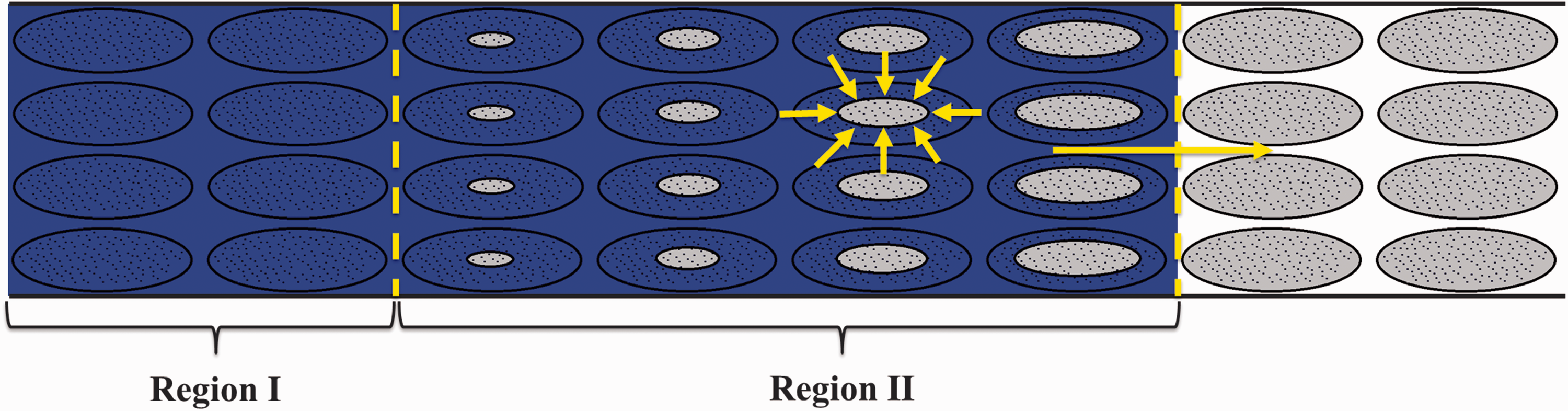
A dual-scale flow occurs when a fluid is injected in a dual-scale porous material. In the case of composites, continuous fiber textiles can be considered as dual-scale porous materials as they are composed of fiber tows, made of hundreds to thousands of fibers, which are woven stitched or braided together. Weaving, stitching or braiding generates macro pores called gaps or channels between the tows. The average size of these gaps is in the range of the millimeter while inside the tows, fibers are separated by some microns to some tens of microns. This bi-dispersed pore size has two consequences on the flow as presented in Figure 1:

It generates an unsaturated region behind the macroscopic flow front (Region II). This unsaturated area presents poor mechanical properties as the tows are not fully saturated. Therefore, its size and position must be predicted accurately in order to ensure that it is resorbed or located in a cut off region of the part at the end of injection.

Resin storage occurs inside the tows, as once the tows are filled there is no more flow inside of them. (Region I). This phenomenon becomes very important in the reactive RTM with online mixing because it implies that the oldest, first injected, resin will be stored in the tows next to the injection point. It may thus affect through exothermic polymerization the temperature and polymerization of the resin injected afterward.

Figure 1.

Unsaturated area in a dual-scale flow.

Thus, classical single-scale simulations are not able to reproduce these two aspects and so may fail to predict what happens finely in the material during injection.

In the next section, the equations governing the flow in the single-scale (Region I and inside of the tows) and dual-scale regions (channels of Region II) will be introduced and numerical techniques developed to simulate the flow in these two types of regions will be presented.

Isothermal flow in a single-scale porous material

Flow of a Newtonian fluid in porous materials has been widely investigated in the past. The commonly used equation to characterize the flow is Darcy’s law (1):¹²

\bar{v} = \frac{- \bar{\bar{K}}}{μ} \bar{\nabla} P

(1)

where,

\bar{v}

is the Darcy velocity of the fluid and P is the pressure in the fluid.

\bar{\bar{K}}

is a tensor containing permeability values. μ is the viscosity of the fluid. The other governing equation for a single-scale fluid flow is the equation of mass balance. It is commonly expressed for an incompressible fluid as (2):

\nabla \cdot \bar{v} = 0

(2)

The pressure profile in the impregnated area can be computed analytically from equations (1) and (2) for 1D linear or radial flow with constant viscosity. However, for 2D impregnations, computational methods are required to access the pressure field and the filling state in the part. Several methods: FEM,¹³ finite difference method⁸ or boundary element method¹⁴ have been proposed in the past to simulate the impregnation of a single-scale porous material. The FEM is nowadays the most used technique and it has been therefore selected in the current work to compute the pressure.

The technique commonly associated with the FEM to track the shape of the impregnated area, is called volume of fluid (VOF). To each node or element of the domain is associated a volume to be filled and a so-called fluid fraction function or fluid filling factor indicating the filling of the control volume. To deal with the filling of the volumes, the velocity of the fluid and the mass balance are used to evaluate the in- and out-flowing volumes from each control volume. In the presented work, the control volumes are the elements themselves and advection equations are used to update the fill factor in the elements.

Isothermal flow in a dual-scale porous material

The most often used technique to deal with a dual-scale flow in complex 2D geometries is the FEM/CV technique presented in the previous section. The major difference is the introduction of a sink term q in the equation of mass balance (2) leading to equation (3).

\nabla \cdot \bar{v} = q

(3)

The sink term q introduces in the mass balance the piece of information that a certain amount of fluid is removed from the macroscopic channels to be stored in the tows. In order to track the fluid filling at the two scales, tows and channels are treated separately. Macroscopic control volumes are dedicated to the flow in the channels and are associated to a microstructure dedicated to the impregnation of the tows. The sink term is then computed from analytical expressions⁷ for simple microstructures or from impregnation simulations conducted on 2D¹⁵ or 3D⁹ unit cell microstructures. The so far developed models use constant tow geometries during the process despite the evolution of the textiles microstructure due to dry or wet decompaction studied in the literature.¹⁶ In Tan and Pillai⁹ and Wang and Grove¹⁵ the impregnation of the microstructures is treated using complex 2D or 3D FEM/CV problems inducing high-computational costs. Moreover, this approach implies to associate one single representative microscopic cell to each node or element of the model. Aside from the fact that the shearing is often not considered in the microstructures, the association one macroscopic element-one microstructure is a high constraint in terms of meshing and implies a high number of elements as unit cells are often not larger than 5 × 5 mm².

In the presented work also, macroscopic and microscopic levels are treated separately using constant tow geometries. However, in order to tackle the highlighted drawbacks of the existing methods, the microstructure associated to each element is adjusted depending on the size, shape, and textile shearing of the macroscopic elements. This makes the method applicable to heterogeneous meshes with element dimensions bigger than one single cell. Moreover, a new microscopic filling strategy has been developed to reduce the time step constraints due to the microscopic filling. Thus the method is supposed to propose a better CPU time efficiency than the methods introduced in Tan and Pillai.^9,11 The details of the method will be presented in the following sections.

Anisothermal flow in a dual-scale porous material

In the case of reactive RTM, chemical reactions occur during filling, generating evolutions in the degree of cure of the resin, coupled with heat generations and modifications of the viscosity. Pillai proposes in Pillai and Jadhav¹⁷ a 2D model to simulate the filling of a single fiber tow, using finite elements to determine the non-isothermal flow of a reactive resin in the channel as well as in the tow. The transfer of the quantities of interest is conducted for each element, using mass, energy, or degree of cure balance. However, the technique is limited to one single tow and the time step used for the computation is strongly constrained by the fixed mesh. In 2010, the Flux Corrected Transport method was adapted by Tan¹¹ to simulate the transport of quantities of interest in the frame of composite molding. This technique is based on the FEM. Values of the quantities of interest (temperature, degree of cure, etc.) are associated to the nodes of the grid and the updated values are obtained from the inversion of a “stiffness matrix”. This iterative method requires many matrix inversions and is therefore CPU time consuming. So as to reduce the calculation time, Abisset-Chavanne⁵ proposed a method inspired from Sanchez¹⁰ based on the VOF method to transport and update the values of the quantities of interest in a single-scale flow. This non-iterative method does not require matrix inversions and appears therefore more CPU time efficient. For this reason, the VOF method will be used in the presented work and adapted to the case of a dual-scale reactive flow.

Numerical developments

Macroscopic and microscopic volume repartition

A macroscopic mesh made of triangular elements covering the whole part allows dealing with the flow in the channels of the material while a representative microstructure is associated to each macroscopic element to deal with the flow in the tows. In the frame of this work, decision has been taken to adapt the microstructure associated to each macroscopic element to the size, shape, and textile shearing of the considered element.

Starting from a given macroscopic mesh, the method used in this paper allows defining an equivalent microstructure associated to each element. This macro–micro association is based on purely geometrical considerations. Tow geometry (cylindrical or rectangular cross-section), tow radius or thickness, inter-tow gap sizes in weft, and warp directions for biaxial textiles as well as fiber orientations (obtained from former draping simulations for example) are considered. Then using the size and shape of the triangular elements of the mesh and the shearing in the element, the number of tows in both directions as well as the average length of tows in both directions is determined in order to maintain the appropriate overall porosity in the element. Additionally, the tows are characterized by their transverse permeability $K_{t}$ computed from Gebart’s law.¹⁸ The volume of the macroscopic (channel) element $V_{macro}$ is computed by removing the volume of tows from the volume of the element (area multiplied by the thickness). Moreover, to each macroscopic element is also associated a permeability tensor ${\bar{\bar{K}}}_{c}$ . The principle of the volume repartition technique is presented in Figure 2.

Figure 2.

Volume repartition: from original material to equivalent tow length and number in the considered element.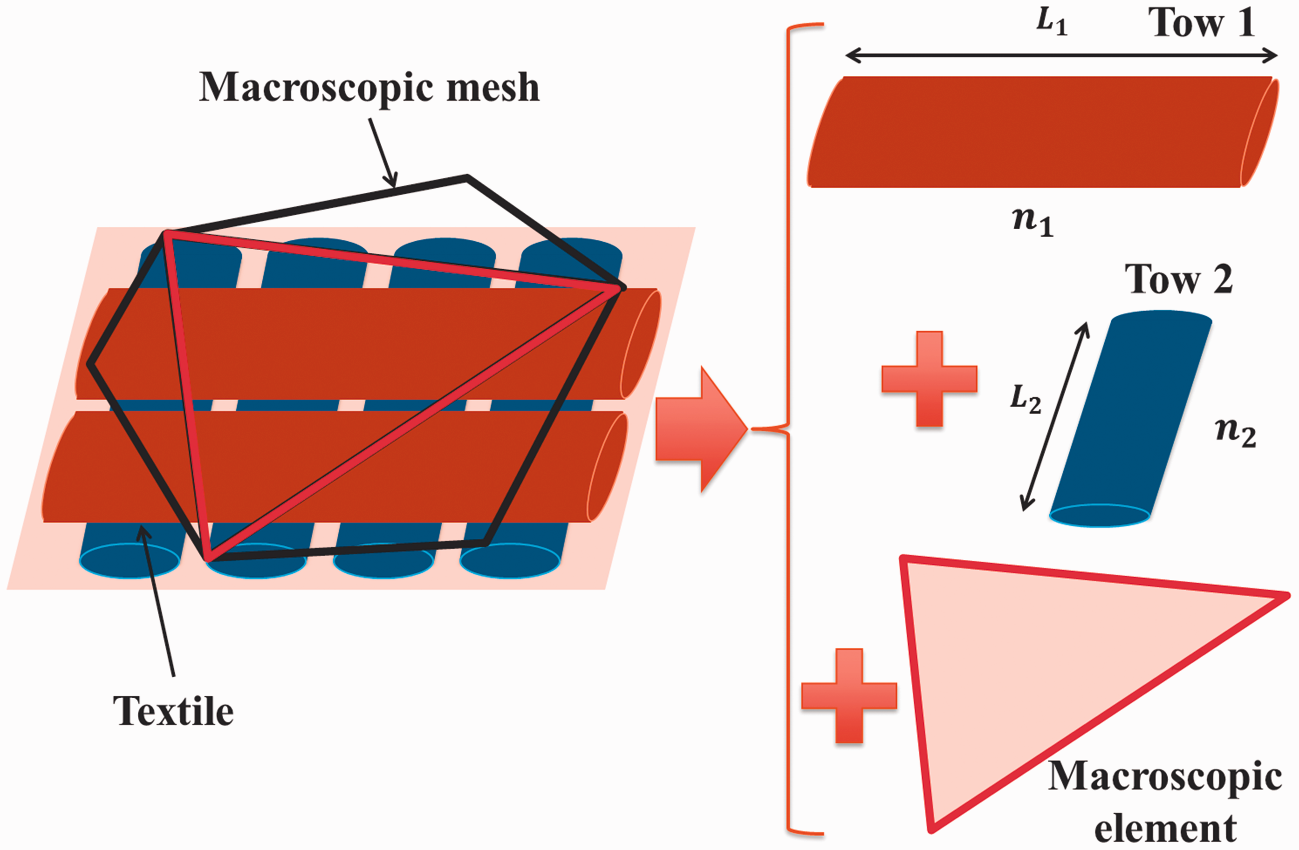

Thanks to this technique, it is therefore possible to determine, for example for a biaxial material, the number and average length of the tows in both directions of the textile whatever size or shape the element may have, the only limitation being the necessity for the element to be larger in both directions than the width of half a tow. The example of a biaxial material will be further considered in this article but the technique is fully applicable for other types of NCFs. During the simulation, all tows in warp and all tows in weft direction will be supposed to fill simultaneously within the same element so that the injection problems will be reduced to two tows: one in each direction. The volumes of fluid absorbed, computed for these two tows, will then be multiplied by the number of tows in both directions in each element and removed from the macroscopic level.

Microscopic tow discretization

As the tows are single-scale porous media, the classical FEM/CV approach is used to compute the pressure and the filling of the microscopic elements. This approach is based on a meshing of the tows. Three assumptions are made regarding tow filling which helps defining the microscopic tow meshing:

In each element, the ratio of tow impregnated surface to the overall tow surface is assumed equal to the macroscopic fluid fraction I_c (Figure 3).

Figure 3.

Ratio equivalence between impregnated to overall volumes, surfaces and lengths.

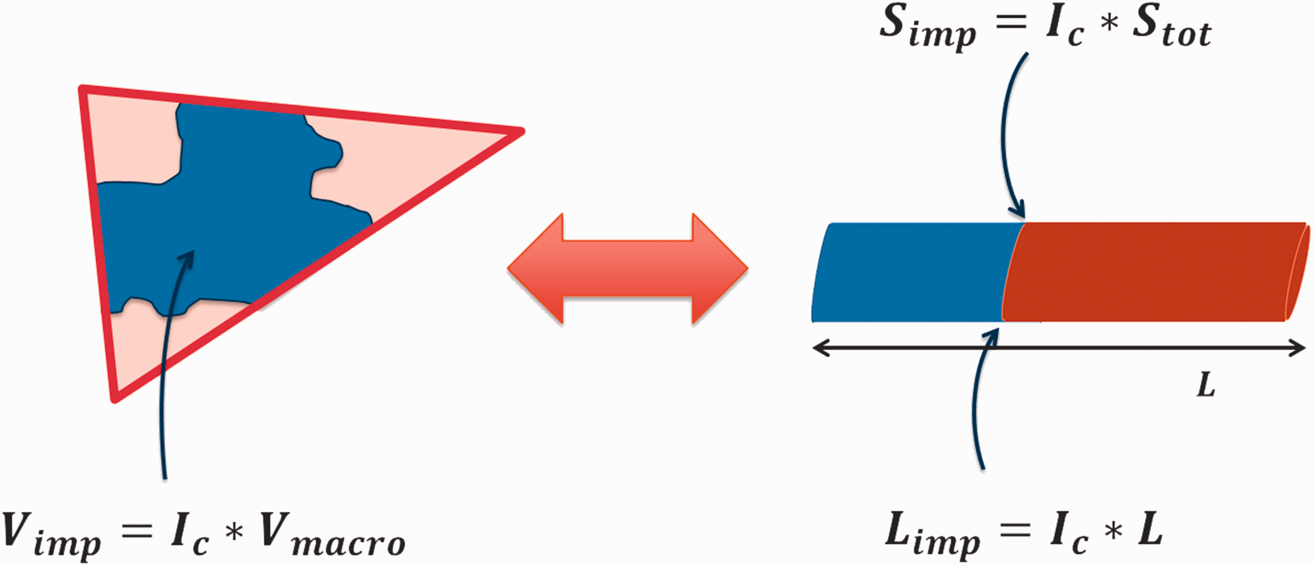
This assumption neglects the influence on the impregnation of the orientation of the flow front relatively to the tows. However, more complex law relating the ratio of volume and the ratio of impregnated surfaces could be introduced to deal with this aspect. Additionally, as the location of the resin in the element is not known, and for sake of simplicity, in the following representations, tow filling will be conducted from one end of the tow. However, it would give identical results starting from any location on the tow. In Figure 3, I_c is the ratio of impregnated volume $V_{imp}$ to the volume of the macroscopic element $V_{macro}$ . It is equal to the ratio of tow impregnated surface $S_{imp}$ to the total tow surface $S_{tot}$ and also to the impregnated length $L_{imp}$ to the total length of the tow L.

Tow filling is assumed to occur exclusively transversely.

For fast injections (less than a few minutes) and high pressures (∼5–30 bar), calculations made on simple cases highlighted that the ratio of longitudinal intra-tow permeability to channel permeability induces a major difference in flow velocities. The longitudinal intra tow flow as well during as after impregnation has been therefore neglected. Therefore the major phenomena generating the impregnation of the tow is the transverse tow filling. Channel permeability to transverse tow permeability ratio has been reported to be in the range of 50–2000,^9,19 for this reason, channels are expected to be filled much faster than the tow so that the tow being impregnated are considered to be surrounded with fluid over their whole periphery. Thus, tow filling problems are reduced to simple 1D filling problems with imposed inlet pressure on the surface of the tow. This pressure is the addition of the channel pressure and the capillary pressure which effects on the transverse flow has been shown to be significant especially at the end of injections conducted at imposed pressures. In the case of cylindrical tows, a radial flow problem is solved, in the case of a rectangular cross-section, the flow problem is solved in the half thickness of the tow.

The tow radius or half thickness cannot be discretized in elements smaller than 10 times the radius of a glass fiber (∼0.15 mm) in the transverse direction.

With this condition, it is assumed that the flow occurs in a homogeneous medium. Therefore Darcy’s equation can be used.

Additionally, as explained in the previous section, the microscopic filling problem in each element can be reduced to two tow filling problems treated separately, one for the warp and one for the weft direction (in the case of a biaxial material). The tow filling problem is presented in Figure 4.

Figure 4.

Microscopic meshing and filling principle of a cylindrical tow with radius R (a) and element thickness dr (b).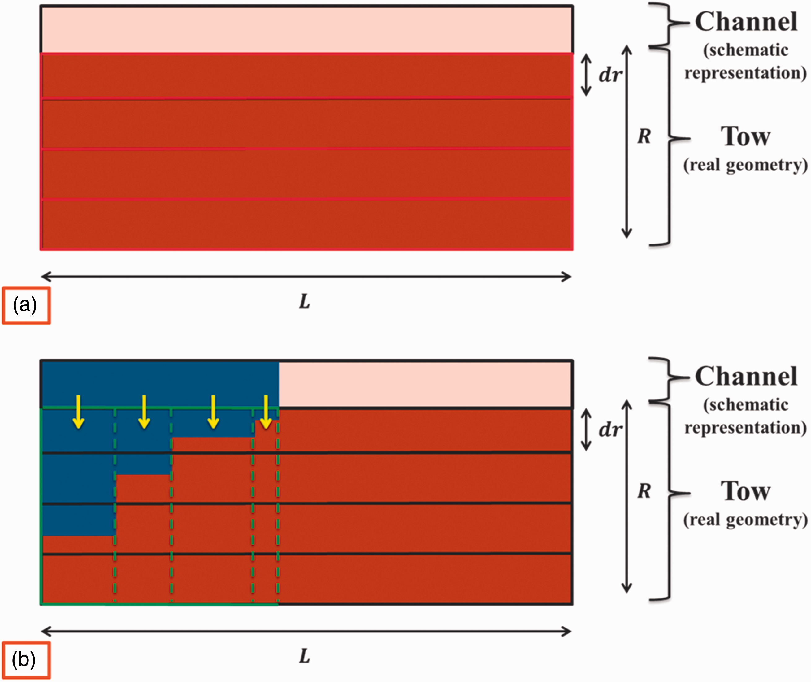

As presented in Figure 4 the discretization of the tow is made both in the transverse (a) and the longitudinal (b) directions. The mesh in the transverse direction is fixed and used for the FEM computation of the pressure field. To each element in the thickness is associated one single value of temperature, degree of cure (and thus of viscosity). Furthermore, a longitudinal mesh will be built along the filling of the macroscopic element (Figure 4(b)) using a numerical method presented in the following section. This longitudinal mesh defines “columns” that will be treated as separated 1D filling problems. These “columns” will allow representing finely the unsaturated area even in elements bigger than this unsaturated area.

The only limitation of this approach is the condition that in each “column”, the fluid should not fill more than the neighbor element of an element containing fluid. This condition is imposed by the VOF method used to compute the values of the quantities of interest in the tows.

This microscopic tow discretization presents the following advantages:

The evolution of the fluid in the longitudinal direction is not limited by any prepositioned mesh.

This makes the approach more flexible in terms of time step definition as there is no limitation of the flow front longitudinal advance within a time step.

The longitudinal discretization and the purely transverse flow assumption reduce the filling problem to a sum of 1D filling problems in each of the “columns”.

This approach is less CPU time consuming than 2D or 3D approaches as the maximal number of 1D pressure field computations to solve is equal to $2 N - 1$ with N the number of microscopic elements in the thickness of the tow (corresponding to the actual flow front position and the flow front located in the neighbor element of the one already impregnated).

The method is applicable whether the elements of the mesh are smaller (Figure 5(a)) or bigger (Figure 5(b)) than the unsaturated area.

Figure 5.

Cases of equivalent tows shorter (a) or longer (b) than the unsaturated area. Both cases can be treated with the proposed method.

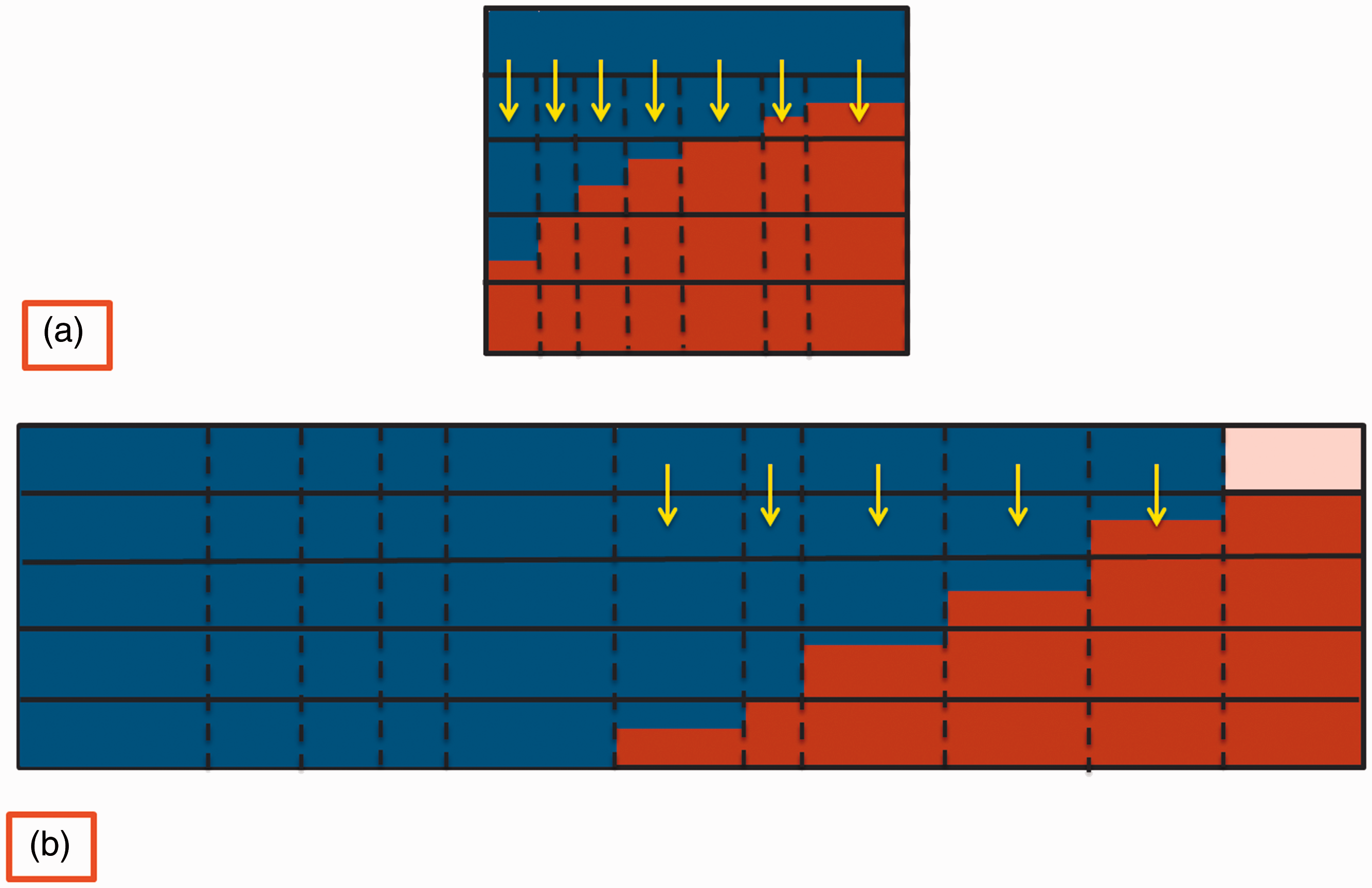
This is a major advantage as the method can be applied to any mesh without caring about the size of the unsaturated area as it would be done for a classical single-scale simulation.

Introduction of the variables

In the following section, the variables will be introduced. In order to differentiate the variables in the channels (macroscopic level) and in the tows (microscopic level), subscripts will be used: c for the channel and t for the tows. For the equations that have the same expression at the macroscopic and microscopic levels, the generic x subscript will be used. Furthermore, the superscript represents the element that is considered: either e for the element itself or $e^{-}$ for the single or multiple upstream elements of element $e .$

As well at the macroscopic as at the microscopic level, the pressure field P_x is defined using pressures values P_i at the nodes of the mesh and linear shape functions $ϕ_{i}$ associated with each node i of the model. The expression of P_x is given in equation (4).

P_{x} = \sum_{i} ϕ_{i} P_{i}

(4)

Furthermore, the following variables are defined and feature constant values in each element that has begun to be filled. It is assumed that, on the inflow boundary of each element, the physical value is equal to the value in the upstream element.

${\bar{v}}_{x}$ : Darcy’s velocity of the fluid in the elemente governed by Darcy’s law (5).

{\bar{v}}_{x}^{e} = \frac{- {\bar{\bar{K}}}_{x}^{e}}{μ_{x}^{e}} \bar{\nabla} P_{x}

(5)

I_x: Fluid fraction in the control volumes.

The fluid fraction function I_x indicates the ratio of the Volume of fluid present in an element, to the overall volume of this element. Moreover, at the macroscopic level, I_c represents the ratio of impregnated surface to the overall exchange surface between the tow and the channel (Figure 3).

The fluid fraction is governed by the advection equation (6) in the whole impregnated domain at both scales.

\frac{\partial I_{x}}{\partial t} + {\bar{v}}_{x} \cdot \bar{\nabla} I_{x} = S_{I}

(6)

Advection equation (6) exhibit a sink term S_I relative to the absorption of fluid in the tows. The generic expression of S_I is given in equation (7) with $Q_{abs}$ the absorption flow rate in the tows and $V_{macro}$ the volume of the macroscopic element.

S_{I} = \frac{Q_{abs}}{V_{macro}}

(7)

S_I is non equal to zero at the macroscopic scale when the tows are being filled and equal to zero when the tows are filled. S_I is also equal to zero at the micro-scale as the flow in the tows is single-scale. The new numerical technique developed in this work to compute S_I in the unsaturated area will be introduced in the following section.

$α_{x} :$ Degree of cure in the elements governed by the advection equation (8) adapted from Abisset-Chavanne and Chinesta.⁵

\frac{\partial α_{x}}{\partial t} + {\bar{v}}_{x} \cdot \bar{\nabla} α_{x} = S_{x}^{polym} - S_{I} α_{c}

(8)

This equation features a source and a sink terms. $S_{x}^{polym}$ is a source term relative to the polymerization of the resin. Among the many models of polymerization presented in the literature, the modified Kamal et al model²⁰ has been chosen in the frame of this work. The expression of $S_{x}^{polym}$ is detailed in equation (9).

K_{i 1}

and

K_{i 2}

are polymerization parameters,

E_{a 1}

and

E_{a 2}

are activation energies of the resin, R is the constant of ideal gases, T_x the temperature of the resin in the channel and m and p experimentally determined parameters. Values for these parameters, taken from Ivankovic et al.,²⁰ are given in Table 1.

Table 1.

Values of the parameters used in the model.²⁰

Parameter	Value
$K_{i 1}$	$e^{10.7} s^{- 1}$
$E_{a 1}$	61.4 kJ/mol
$K_{i 2}$	$e^{12.6} s^{- 1}$
$E_{a 2}$	62.1 kJ/mol
m	0.64
p	1.36
R	8.314 J/mol/K
$α_{\max}$	−1.43 + 0.00591 × T
ΔH	365 × 10₃J/kg
$ρ^{r}$	1028 kg/m³
$ρ^{t}$	2560 kg/m³
$ɛ_{c}$	1
$ɛ_{t}$	0.4
$C_{p}^{r}$	1500 J/K/kg
$k^{r}$	0.24 W/m/K
$C_{p}^{f}$ (Glass fiber)	670 J/K/kg
$k^{f}$ (Glass fiber)	0.0335 W/m/K
$μ_{g}$	$10^{12}$ Pa s
C ₁	36.5
C ₂	19.6
$T_{g 0}$	235.4 K
$α_{g}$	0.331
$n_{μ}$	2.7

Moreover, $S_{I} α_{c}$ is the sink term non equal to zero in the unsaturated area relative to the absorption of fluid with a certain degree of polymerization in the tows. This is the only contribution of the tows to the evolution of the polymerization in the channel as the tow is not supposed to influence chemically the polymerization reaction.

T_x: Temperature in the elements governed by the advection equation (10) also called equation of heat.

ρ^{x} C_{p}^{x} (\frac{\partial T_{x}}{\partial t} + {\bar{v}}_{x} \cdot \bar{\nabla} T_{x}) = S_{T}^{cond} + S_{T}^{polym} + S_{T}^{micro} - S_{I} T_{c}

(10)

In this equation, $ρ^{x}$ is the average density at the considered scale and $C_{p}^{x}$ is the average heat capacity. These two values are assumed constant. In the channel, $ρ^{c} C_{p}^{c} = ρ^{r} C_{p}^{r}$ where r stands for the properties of the resin and in the tow, $ρ^{x} C_{p}^{x} = ϕ_{t} ρ^{r} C_{p}^{r} + (1 - ϕ_{t}) ρ^{f} C_{p}^{f}$ where $ϕ_{t}$ is the porosity in the tow and f stands for the properties of the fibers (Table 1). $S_{T}^{cond}$ is a source or sink term relative to the conductive thermal exchanges between the elements and is defined in equation (11).

S_{T}^{cond} = k^{x} Δ T_{x}

(11)

$k^{x}$ is the thermal conductivity in the considered region

$S_{T}^{polym}$ is defined in equation (12).

S_{T}^{polym} = ρ^{r} ɛ_{x} Δ H \frac{\partial α_{x}}{\partial t}

(12)

$ɛ_{x}$ is the porosity at the considered scale and $Δ H$ is the heat generated by the curing reaction (Table 1).

$S_{T}^{micro}$ is the source or sink term relative to the conductive thermal exchanges between the tow and the channel. It is computed as the conductive exchanges of the cylindrical tow surrounded by fluid flowing in the channel. Furthermore, $S_{I} T_{c}$ is the sink term relative to the absorption of fluid with a certain temperature in the tow. Both terms are constantly computed and taken into account in the equation, however, their relative influence depends on time: $S_{T}^{micro}$ has a negligible influence during tow filling but becomes significant when the advective term $S_{I} T_{c}$ vanishes once the tow is filled.

It can be noted that both temperature and degree of cure, follow advection equations in the form of (13) where J_x is a generic quantity of interest. Therefore, to simplify the following explanations regarding reactive aspects, equation (13) will be used to explain how the evolution of temperature and degree of cure are treated numerically. S_J is a generic expression for sink or source term(s) relative to the considered quantity of interest. C is a generic expression for the coefficient multiplying the right hand side terms of advection equations.

C (\frac{\partial J_{x}}{\partial t} + {\bar{v}}_{x} \cdot \bar{\nabla} J_{x}) = S_{J} - S_{I} J_{c}

(13)

$μ_{x}$ : Viscosity of the fluid governed by the chemo-thermo-rheological law (16) taken from Ivankovic et al.²⁰

μ_{x} = μ_{g} exp [\frac{C_{1} (T_{x} - T_{g 0})}{C_{2} + T_{x} - T_{g 0}}] (\frac{α_{g}}{α_{g} - α_{x}})^{n_{μ}}

(14)

In equation (14), $T_{g 0}$ is the glass transition temperature of the uncured resin, $μ_{g}$ is the viscosity at $T_{g 0}$ and $α_{g}$ the degree of cure at the gelation point. C₁, C₂, and $n_{μ}$ are constants. Values of these parameters are given in Table 1.

General algorithm

Time step definition

Two conditions must be satisfied to enable the use of the presented technique:

No overfilling may occur at the macroscopic scale.

Therefore, the time step must be chosen so that equation (15) is satisfied:

I_{c}^{n + 1} - I_{c}^{n} \leq (1 - I_{th})

(15)

In equation (15) I_th is a number close to one. Once the fluid fraction in an element has reached I_th the element is considered as filled.

No more than one element may be filled in the transverse direction of the tows at the microscopic scale.

The simplified expression that the time step Δt must satisfy is presented in equation (16):

Δ t < \frac{Δ z^{2} μ_{c}}{P_{av} K_{t}}

(16)

In equation (16), Δz is the tow transverse discretization size and $P_{av}$ the average pressure over the three nodes of the macroscopic element that is used as boundary condition for the tow filling problem.

The smallest time step obtained from these two criteria is used for the calculation.

Macroscopic pressure field and flow velocity determination

The first step of the numerical strategy consists in computing the macroscopic pressure field in the impregnated area. Equations (1) and (3) are combined. The sink term has the same expression as S_I(defined in equation (7)).

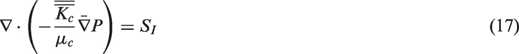
\nabla \cdot (- \frac{\bar{\bar{K_{c}}}}{μ_{c}} \bar{\nabla} P) = S_{I}

(17)

The pressure field is computed using the variational formulation of equation (17) and the boundary conditions. From this pressure field, upstream and downstream elements are determined for each element of the impregnated area. Then, using Darcy’s law (1) and the pressure at the nodes of each element, the velocity of the fluid is computed in each element of the impregnated area. From these flow velocities and the list of upstream and downstream elements, the amount of fluid flowing in and out of each macroscopic element during the considered time step is computed.

Macroscopic and microscopic filling

Considering the element $e_{macro}$ with $n 1$ tows in direction 1 and $n 2$ tows in direction 2; tows in direction 1 have the average length L₁ and tows in direction 2 the average length L₂.

As explained in the previous section, a result of the macroscopic pressure and flow velocity determination is the amount of fluid $V_{in}$ coming in the considered element during a considered time step. This volume needs to be shared between the macroscopic and the microscopic scales. In fact, a position of equilibrium for the macroscopic flow front can be determined analytically so that both Darcy’s flow in the tow and mass balance for the repartition of $V_{in}$ between the two scales can be satisfied.

First time step of the elements filling. When fluid arrives for the first time in an element, the repartition of the volume $V_{in}$ between the macroscopic and microscopic levels requires determining:

The position in the thickness of the tow that will be reached by the microscopic flow front during the time step due to Darcy’s flow.

The increase in impregnated tow surface (corresponding to the longitudinal propagation of the flow front) during this time step.

These two problems are solved analytically using the following processes:

Flow front position in the thickness of the tow. A simple 1D filling problem is solved to determine the position reached in the thickness of the tow during the purely transverse filling. The average pressure over the three nodes of the macroscopic element added to the capillary pressure computed from the expression given by Ahn²¹ is used as boundary condition. Using the transverse discretization of the tow, the pressure field is computed as well as the flow velocity using Darcy’s equation (1). The duration of the time step allows determining the volumes V₁ and V₂ of fluid that would be absorbed through the entire surface of one tow in direction 1 ( $S_{tot 1}$ ) and in direction 2 ( $S_{tot 2}$ ). Thus the volumes of fluid really absorbed in tows 1 and 2 during the time step are, respectively, $V_{1} (S_{imp 1} / S_{tot 1}) n_{1}$ and $V_{2} (S_{imp 2} / S_{tot 2}) n_{2}$ with $S_{imp 1}$ and $S_{imp 2}$ the exchange, impregnated, surfaces between channel and tows 1 and 2. $S_{imp 1}$ and $S_{imp 2}$ needs to be determined.

Impregnated tow surface determination. The volume injected in the element V_in needs to be shared between the channel and the tow satisfying mass balance. Its repartition satisfies equation (18).

V_{in} = V_{1} \frac{S_{imp 1}}{S_{tot 1}} n_{1} + V_{2} \frac{S_{imp 2}}{S_{tot 2}} n_{2} + V_{c}

(18)

In equation (18) V_c is the Volume of fluid remaining in the channel.

Assuming that $I_{c} = \frac{S_{imp 1}}{S_{tot 1}} = \frac{S_{imp 2}}{S_{tot 2}}$ and $V_{c} = \frac{V_{c}}{V_{macro}} V_{macro} = I_{c} V_{macro}$ equation (18) can be rewritten as equation (19).

V_{in} = V_{1} n_{1} I_{c} + V_{2} n_{2} I_{c} + I_{c} V_{macro}

(19)

Therefore, the new filling state $I_{c}^{n + 1}$ of the element can be computed using equation (20).

I_{c}^{n + 1} = \frac{V_{in}}{V_{1} n_{1} + V_{2} n_{2} + V_{macro}}

(20)

It allows accessing the new exchange surface $S_{imp}^{n + 1} = I_{c}^{n + 1} S_{tot}$ and the longitudinal length of the first column: $I_{c}^{n + 1} L_{1}$ in the tow 1 and $I_{c}^{n + 1} L_{2}$ in the tow 2. These lengths are saved to be used at the following time step.

In the newly generated column, the filling state of the microscopic elements is updated using equation (6). In practice, to compute 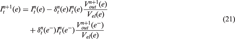$I_{t},$ the weak form of equation (6) is integrated and expressed using a first order explicit approximation of the time derivative. Moreover, as proposed in Sanchez et al.,¹⁰ the test function $δ_{x}$ is introduced in the equation in order to avoid diffusion of the macroscopic flow front ( $δ_{x} = 1$ if the element eis numerically considered as filled, $δ_{x} = 0$ in the other cases). Equation (7) is obtained.

I_{t}^{n + 1} (e) = I_{t}^{n} (e) - δ_{t}^{n} (e) I_{t}^{n} (e) \frac{V_{out}^{n + 1} (e)}{V_{el} (e)} + δ_{t}^{n} (e^{-}) I_{t}^{n} (e^{-}) \frac{V_{out}^{n + 1} (e^{-})}{V_{el} (e)}

(21)

In this equation, $V_{out}^{n + 1} (e)$ is the volume flowing out of the element e of the considered column at time step $n + 1$ calculated from fluid velocity in e. $e^{-}$ is the upstream element of elemente thus, $V_{out}^{n + 1} (e^{-})$ is the overall volume coming in the elemente at time step $n + 1$ . $V_{el} (e)$ is the volume of the element e in the considered column.

The flow front position in the column is saved for the future pressure field computation as well as the filling factor of the element where the flow front is located for the future update of the filling. Additionally, the volume absorbed in the tows is saved to compute S_I using equation (7). Finally, the volumes exchanged between the longitudinal elements are computed from the volumes exchanged in each column. Furthermore, the filling state of the longitudinal elements is calculated using the appropriate expression of equation (6). Exchanged volumes and filling factor are used to update the reaction related quantities of interest.

Following time steps. Once the first column has been generated, the approach is the same for two or more columns. The longitudinal length of each existing column is known. Thus, in these columns, the volume absorbed is computed directly using Darcy’s law and removed from the volume $V_{in}$ introduced in the element. Once the contribution of all columns has been taken into account, the remaining volume of fluid is shared between the channel and the tow using the same procedure as for the first column.

In this case, longitudinal length of the microscopic “column” created during the time step n + 1 in each tow is expressed as follows: ( $I_{c}^{n + 1} - I_{c}^{n}) L_{i}$ . The same information as for the first filling time step are saved regarding flow front position and filling state in the columns as well as their overall values in the longitudinal elements.

Once the level of filling at the macroscopic scale has reached 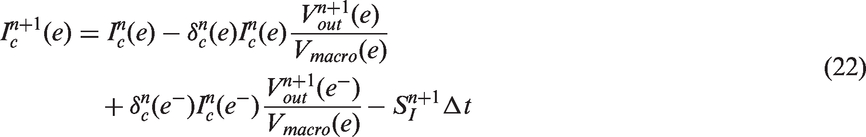$I_{th}$ , macroscopic flow is allowed in the downstream elements, the tows continue being filled using the same microscopic approach to compute S_I and the filling state I_c is updated using equation (22) obtained in a similar way as equation (21).

I_{c}^{n + 1} (e) = I_{c}^{n} (e) - δ_{c}^{n} (e) I_{c}^{n} (e) \frac{V_{out}^{n + 1} (e)}{V_{macro} (e)} + δ_{c}^{n} (e^{-}) I_{c}^{n} (e^{-}) \frac{V_{out}^{n + 1} (e^{-})}{V_{macro} (e)} - S_{I}^{n + 1} Δ t

(22)

Updating the other quantities of interest

Unlike the filling problem, for which a fine description is required to determine precisely the sink term and track the size of the unsaturated area, the choice have been made to consider one single value of temperature and degree of cure in each of the longitudinal elements of the tows.

As described in the previous section, temperature and degree of cure are governed by equations in the form of equation (13). With the approach developed by Abisset-Chavanne,⁵ adapted to the case of the dual-scale flow, equation (13) can be rewritten using a first order explicit approximation of the time derivative. Equation (23) is obtained.

J_{x}^{n + 1} (e) = \frac{1}{I_{x}^{n + 1} (e)} [I_{x}^{n} (e) {\tilde{J_{x}}}^{n + 1} (e) - δ_{x}^{n} (e) {\tilde{J_{x}}}^{n + 1} (e) \frac{V_{out}^{n + 1} (e)}{V_{el} (e)} + δ_{x}^{n} (e^{-}) {\tilde{J_{x}}}^{n + 1} (e^{-}) \frac{V_{out}^{n + 1} (e^{-})}{V_{el} (e)} {\tilde{J_{x}}}^{n + 1} (e) S_{I}^{n + 1} (e) Δ t]

(23)

${\tilde{J_{x}}}^{n + 1} (e)$ takes the non-convective source terms of equation (13) into account. It is defined in equation (24):

{\tilde{J_{x}}}^{n + 1} (e) = J_{c}^{n} (e) + \frac{S_{J}^{n + 1} (e) Δ t}{C}

(24)

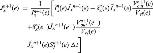
Equation (23) can be directly used at the macro-scale. However, specific attention must be paid to the microscopic level. In fact, when the tow finishes being filled, fully filled columns and partially filled columns cohabit in the element. Therefore, treatment of the advection equation must be adapted. Figure 6 illustrates the problem.

Figure 6.

Example of tow where cohabit filled and unfilled columns.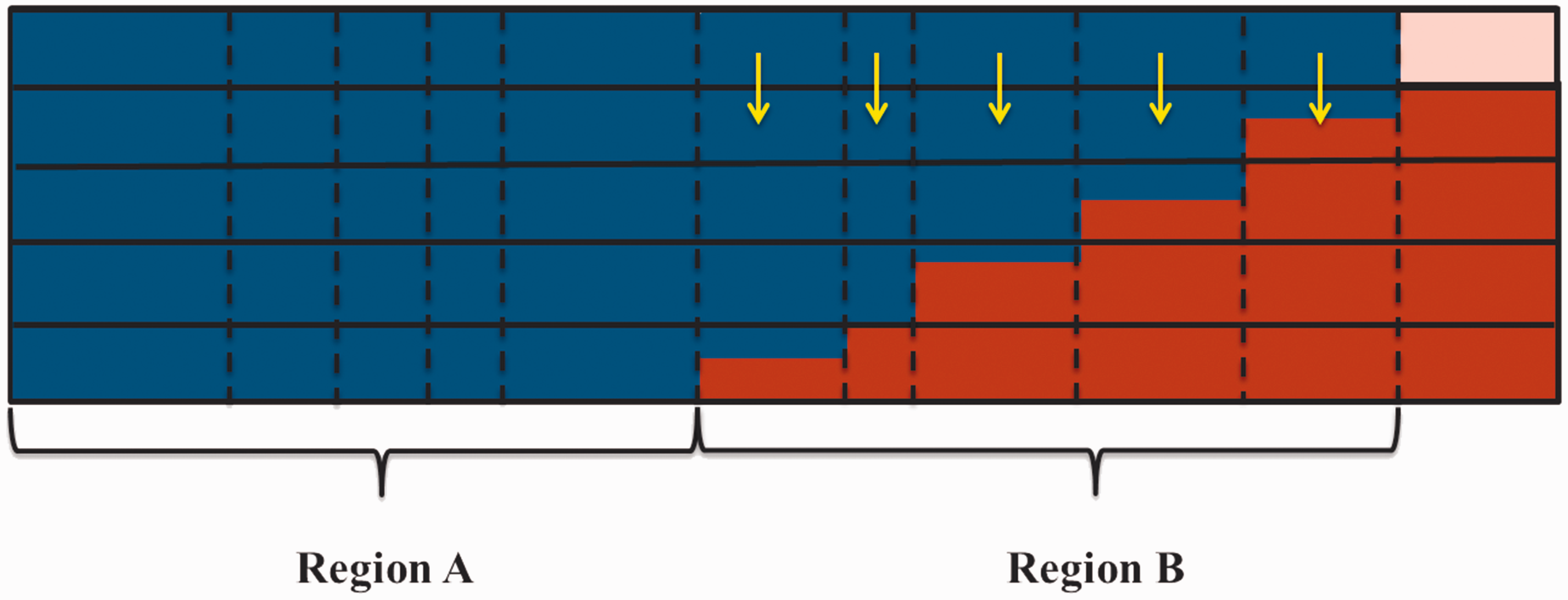

The longitudinal elements are split in two regions. In region A where the resin is stored, the convective terms of equation (23) must be removed from the computation. In region B, flow still occurs in the columns. Therefore, equation (23) including convective terms is used. Furthermore, it is considered that the only exchanges between region A and B is the inclusion in region A of the columns after their fulfilling. Thus two values of temperature and degree of cure are computed in each longitudinal element, one in each region. Finally to propose a unique value of temperature or degree of cure over the whole longitudinal elements, a volume average of the quantities of interest is computed.

Once the quantities of interest relative to the reactive character of the injection have been computed, viscosity is computed in each element using equation (14) and a new time step can be started.

Numerical examples

In this section, unidirectional filling simulations of a rectangular cavity containing a dual-scale porous material will be presented to highlight the characteristics of the developed method.

Isothermal filling simulation: flexibility of the method regarding mesh size and textile properties

One of the claims of the developed technique is that it is able to treat dual-scale flow with the same degree of precision with various element sizes. Therefore, isothermal 1D filling simulations with constant inlet pressure have been conducted using meshes with element sizes from 2 to 20 mm. Different values of material properties have also been considered in order to determine the sensitivity of the method to the relative size of the channels to the overall volume of the part (

ϕ_{c})

or the channel to transverse tow permeability ratio (K_c/K_t). The tows are considered cylindrical and exhibit a constant geometry and a constant intra-tow porosity equal to 0.4. Therefore, the evolutions of

ϕ_{c}

and the average porosity are only due to the increase of the size of the channels. The characteristics of the textile and the processing conditions are described in Table 2.

Table 2.

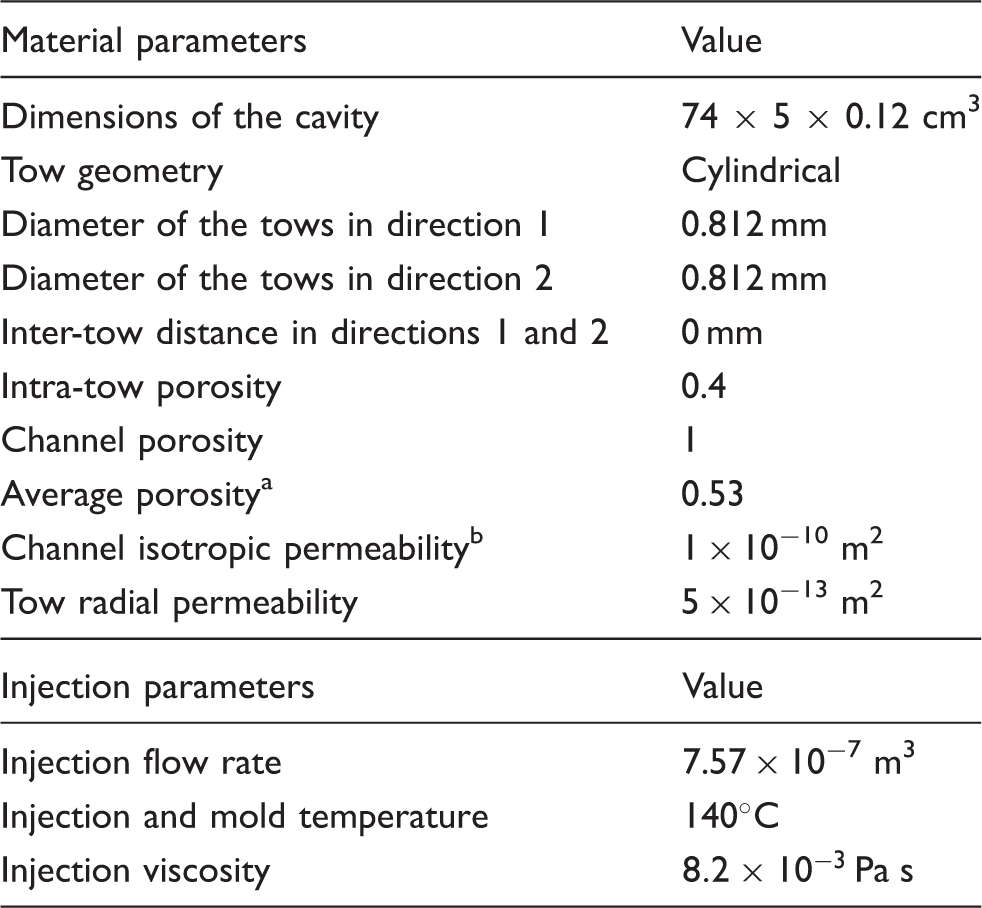
Textile parameters and processing conditions used for the different pressure imposed isothermal filling simulations

Material parameters	Values
Length of the cavity		20 cm
Diameter of the tows in direction 1		0.812 mm
Diameter of the tows in direction 2		0.812 mm
Channel to overall volume ratio ( $ϕ_{c}$ )	0.13	0.26	0.40
Average porosity	0.48	0.55	0.64
Channel isotropic permeability		$10^{- 10}$ m²
Tow radial permeability	$1 \times 10^{- 13}$ m²	$5 \times 10^{- 13}$ m²	$5 \times 10^{- 12}$ m²
Injection parameters		Value
Injection pressure		10⁵Pa
Injection viscosity		$8.2 \times 10^{- 3}$ Pa s

Additionally, as presented in section “Macroscopic and microscopic volume repartition”, the size and length of the tows associated to each macroscopic element depend on the characteristics of the considered material and the size of the element itself. The values and average length of tows in the elements depending on the size of the elements and

ϕ_{c}

are thus presented in Table 3.

Table 3.

Number and average length of tows in both directions depending on the element size and the channel to overall volume ratio $ϕ_{c}$ .

Macroscopic mesh	$ϕ_{c}$ = 0.13				$ϕ_{c}$ = 0.26				$ϕ_{c}$ = 0.40
Macroscopic mesh	2 mm	5 mm	10 mm	20 mm	2 mm	5 mm	10 mm	20 mm	2 mm	5 mm	10 mm	20 mm
Number of tows in direction 1	0.5	1.5	3	6	0.5	1.5	3	6	0.5	1	2.5	4.5
Tow average length direction 1	1.2 mm	2.6 mm	5.1 mm	10.3 mm	1.2 mm	2.4 mm	4.8 mm	9.7 mm	1.2 mm	2.9 mm	4.7 mm	10.5 mm
Number of tows in direction 2	1	3	6	12.5	1	3	6	11.5	1	2.5	4.5	9.5
Tow average length direction 2	0.6 mm	1.3 mm	2.6 mm	4.9 mm	0.6 mm	1.2 mm	2.4 mm	5 mm	0.6 mm	1.2 mm	2.6 mm	5 mm

Two types of results will be presented: first, the injected volume versus time will be compared for the different scenarii. This result is a direct representation of the flow front propagation and tow impregnation as they both influence the flow velocity in the part and thus the injected volume. Second, the length of the unsaturated area will be compared for the reference case (K_c/K_t = 200, $ϕ_{c}$ = 0.26) in order to highlight the ability for the model to reproduce the unsaturated area in the same way for different sizes of meshes. One-dimensional injections with constant pressure equal to $10^{5}$ Pa are conducted. The reference time to compare the different simulations is the time necessary to fill one half of the volume of the cavity (1D flow over 10 cm). For the considered injection pressure and channel permeability, the average flow velocity during impregnation is in the range of 4 cm per second and the smallest flow velocity at the end of injection is 1.2 cm/s. Thus the flow regime is in the range of the ones observed in high pressure RTM. Figure 7 presents results obtained for mesh sizes comprises between 2 and 20 mm, with the K_c/K_t = 200, $ϕ_{c}$ = 0.26). The reference volume for the volume normalization in Figure 7 is one half the volume of the cavity.

Figure 7.

Influence of mesh size on the normalized injected volume versus time for an isothermal injection with constant injection pressure.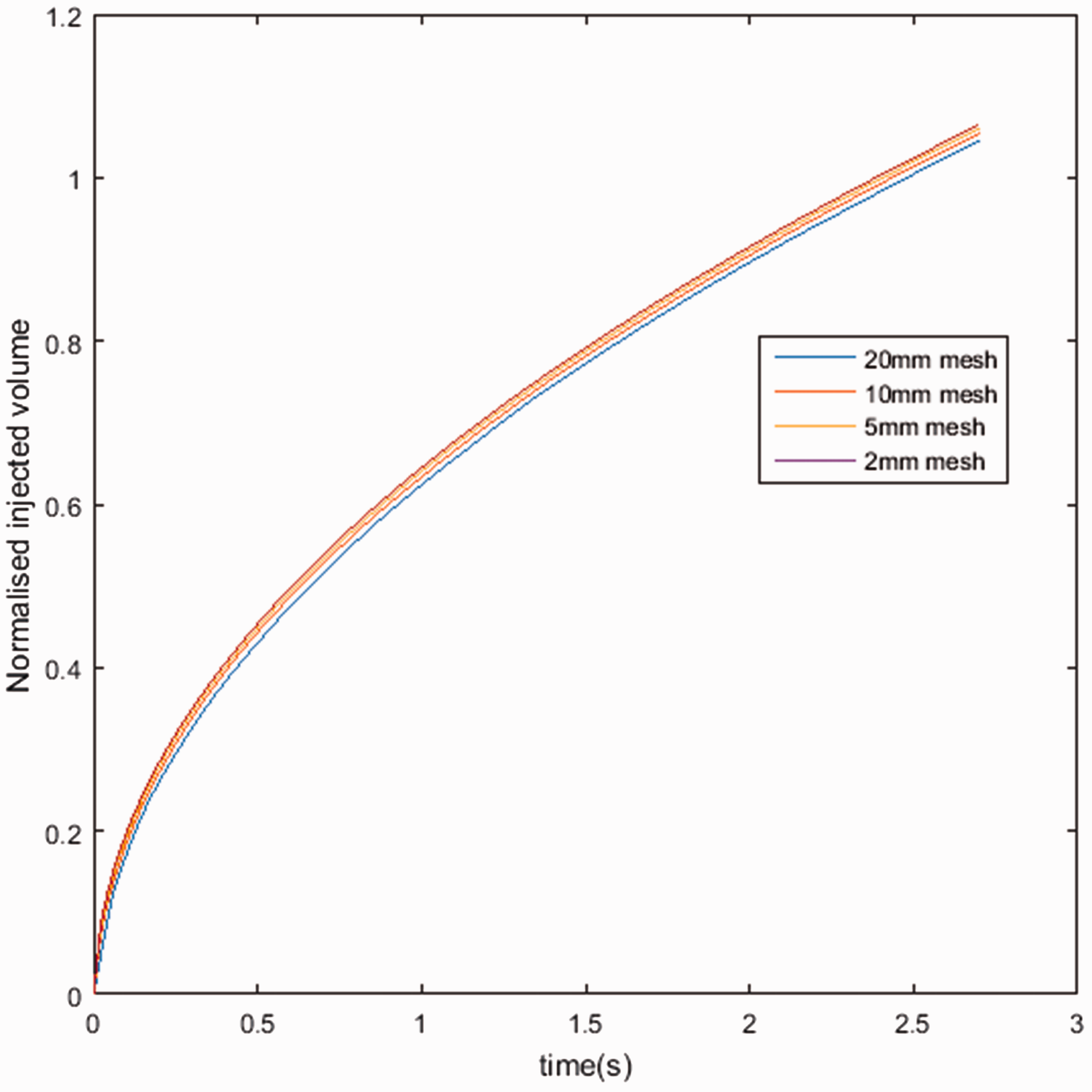

It can be observed that the plots of injected volume versus time are very close to each other for the four elements sizes. Table 4 gives the numerical values of injection times for the different scenario. In each cases, the injection time is compared to the time obtained from the most refined 2 mm mesh simulation.

Table 4.

Computed injection times for the different scenario and errors to the results obtained from the 2 mm mesh calculations.

Mesh size (mm)	Time to fill ½ of the cavity (s)	Error to 2 mm mesh (%)	Mesh size (mm)	Time to fill ½ of the cavity (s)	Error to 2 mm mesh (%)	Mesh size (mm)	Time to fill ½ of the cavity (s)	Error to 2 mm mesh (%)
K_c/K_t = 1000, $ϕ_{c}$ = 0.26			K_c/K_t = 200, $ϕ_{c}$ = 0.26			K_c/K_t = 20, $ϕ_{c}$ = 0.26
2	2.41		2	2.38		2	2.38
5	2.44	1.24	5	2.40	0.84	5	2.38	0
10	2.48	2.9	10	2.43	2.1	10	2.42	1.68
20	2.53	5.0	20	2.47	3.78	20	2.47	3.78
K_c/K_t = 200, $ϕ_{c}$ = 0.13			K_c/K_t = 200, $ϕ_{c}$ = 0.26			K_c/K_t = 200, $ϕ_{c}$ = 0.40
2	2.06		2	2.38		2	2.72
5	2.06	0	5	2.40	0.84	5	2.76	1.47
10	2.08	0.9	10	2.43	2.1	10	2.80	2.94
20	2.1	1.9	20	2.47	3.78	20	2.88	5.88

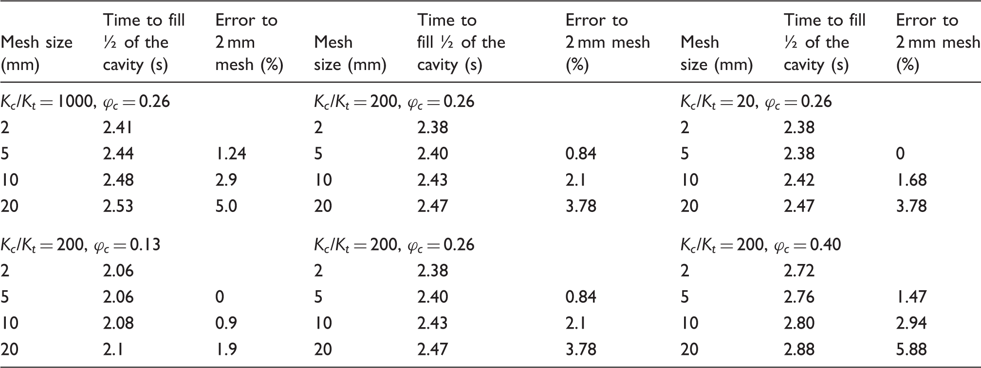
It can be noticed from Table 4 that with increasing mesh size, the error on the injection time is increasing. However, even when dividing the number of macroscopic elements in the model by a factor 10, this error remains under 6%. This demonstrates the flexibility of the proposed model and its ability to treat equivalently an isothermal injection case for several element sizes.

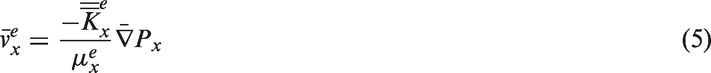
Additionally, the size of the unsaturated area has been compared for the different mesh sizes for the reference case (K_c/K_t = 200, $ϕ_{c}$ = 0.26). Figure 8 presents the filling state of the part after 2 s of injection. I_c represents the level of filling at the macroscopic scale while I_t presents the level of filling of the tows. It can be noticed that with the 2 mm mesh, the unsaturated area can be well observed as the elements are smaller than the unsaturated area. Its length is estimated to 9 mm. The bigger the elements of the mesh, the more difficult it is to notice the unsaturated area as it is spread over a smaller number of elements or is even smaller than the element itself. However, its size can be determined using the microscopic model. In the case of the 20 mm large mesh, the average length of unsaturated area during injection is 9.25 mm. This value is very close to the length of unsaturated area that can be measured from the more discretized 2 mm mesh simulation. This highlights the capacity for the model to track finely the unsaturated area even with large elements.

Figure 8.

Isothermal 1D filling simulation under the same conditions with varying mesh sizes. Filling state at the macroscopic (I_c) and microscopic (I_t) levels.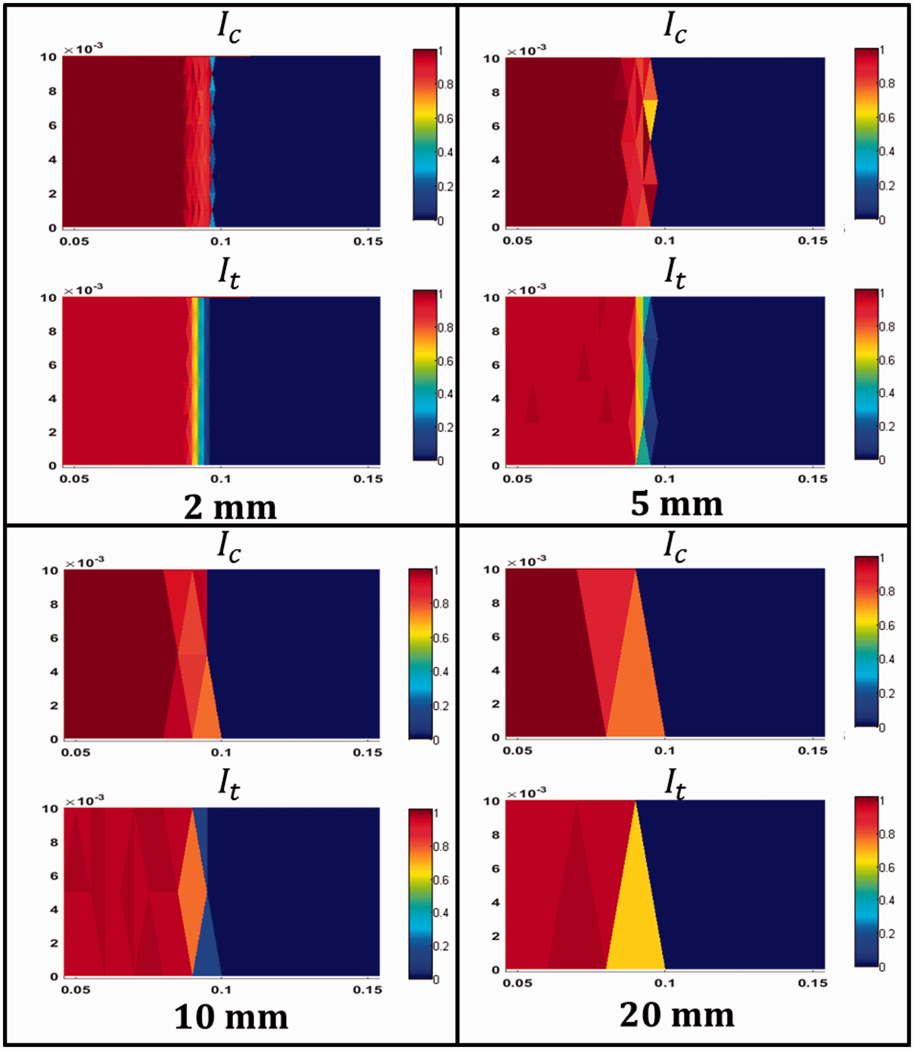

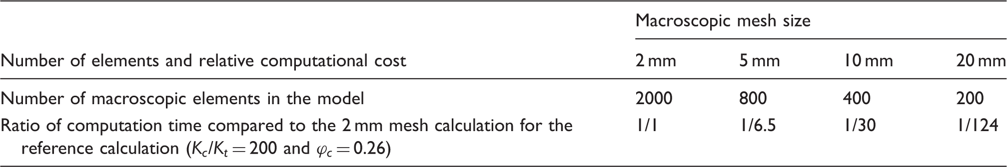
Finally, Table 5 presents the advantages of the new numerical method in terms of CPU time reduction for the reference calculation. In the case of the 20 mm mesh, the computation time is reduced by a factor 124 while the error on the filling time stays smaller than 5% compared to the 2 mm mesh. These results highlight therefore that the model can be run with the same degree of accuracy with various element sizes. This may enable time savings both at the meshing step, as elements with sizes between 2 and 20 mm generate equivalent results, and at the calculation step, as larger elements can be used, which allow reducing the number of elements and thus the CPU time.

Table 5.

Number of elements and relative computational cost for the reference case treated with different element sizes.

Number of elements and relative computational cost	Macroscopic mesh size
Number of elements and relative computational cost	2 mm	5 mm	10 mm	20 mm
Number of macroscopic elements in the model	2000	800	400	200
Ratio of computation time compared to the 2 mm mesh calculation for the reference calculation (K_c/K_t = 200 and $ϕ_{c}$ = 0.26)	1/1	1/6.5	1/30	1/124

Dual-scale reactive simulation under constant injection flow rate

A single-scale reactive simulation using parameters of Table 6 has shown that the resin reaches the outlet after 84 s and prior to gelling. A dual-scale simulation is then conducted using the same material and injection parameters. Injection is stopped after 84s. Mappings of the fluid fraction, the degree of cure, the temperature and the viscosity after 84s seconds of injection are presented in Figure 9. Furthermore, figure 10 presents the evolution of the injection pressure with respect to the time.

Table 6.

Parameters used for the reactive single and dual-scale 1D filling simulations.

Material parameters	Value
Dimensions of the cavity	74 × 5 × 0.12 cm³
Tow geometry	Cylindrical
Diameter of the tows in direction 1	0.812 mm
Diameter of the tows in direction 2	0.812 mm
Inter-tow distance in directions 1 and 2	0 mm
Intra-tow porosity	0.4
Channel porosity	1
Average porosity^a	0.53
Channel isotropic permeability^b	1 × 10⁻¹⁰ m²
Tow radial permeability	5 × 10⁻¹³ m²

Injection parameters	Value
Injection flow rate	7.57 × 10⁻⁷ m³
Injection and mold temperature	$140 \deg C$
Injection viscosity	$8.2 \times 10^{- 3} Pas$

Porosity used for the single-scale simulation.

Permeability used for the single-scale and the channels of the dual-scale simulation.

Figure 9.

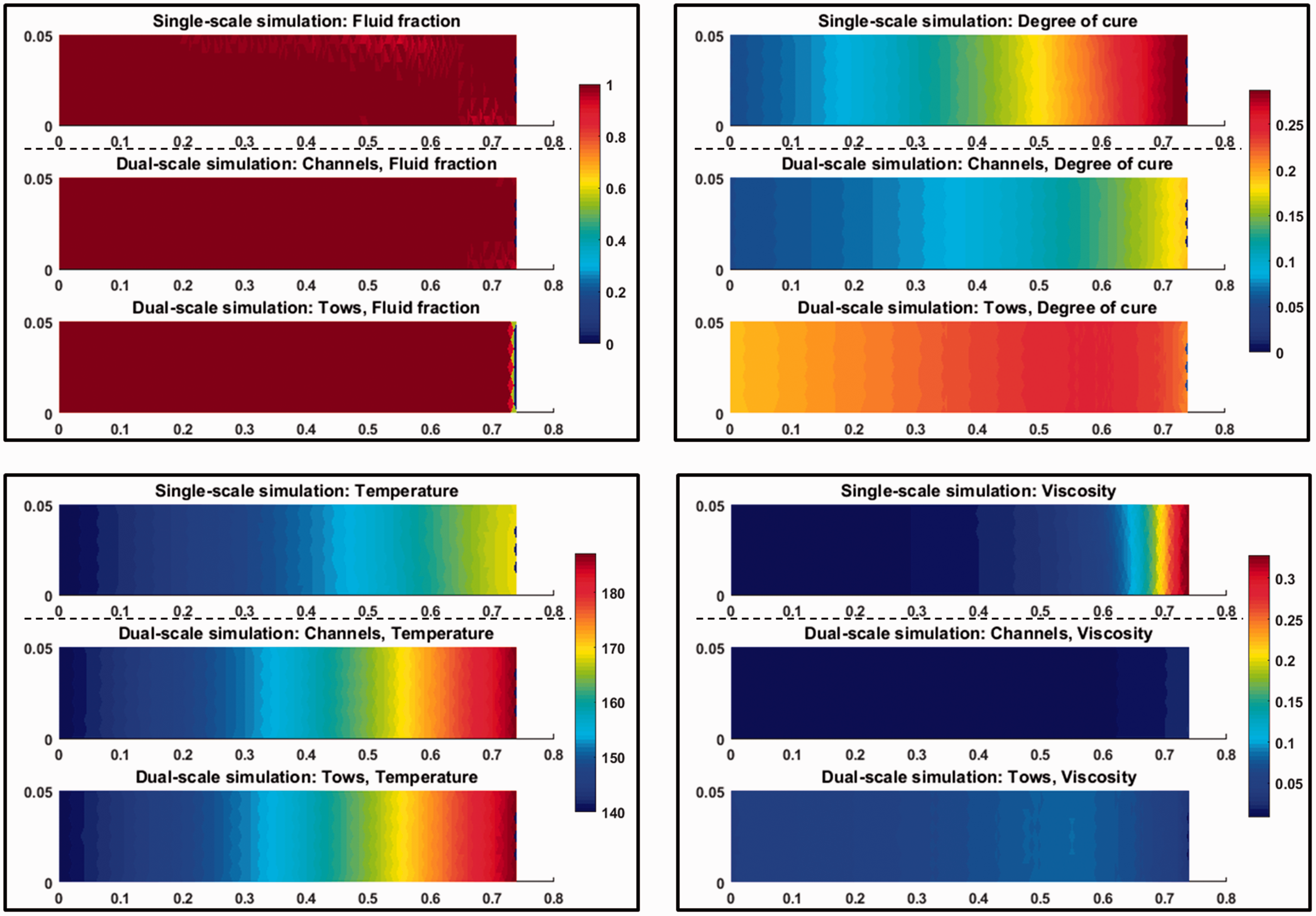
Comparison of single and dual-scale reactive simulations results using the same material and injection parameters. Quantities of interest: fluid fraction, degree of cure, temperature (℃) and viscosity (Pa s).

Figure 10.

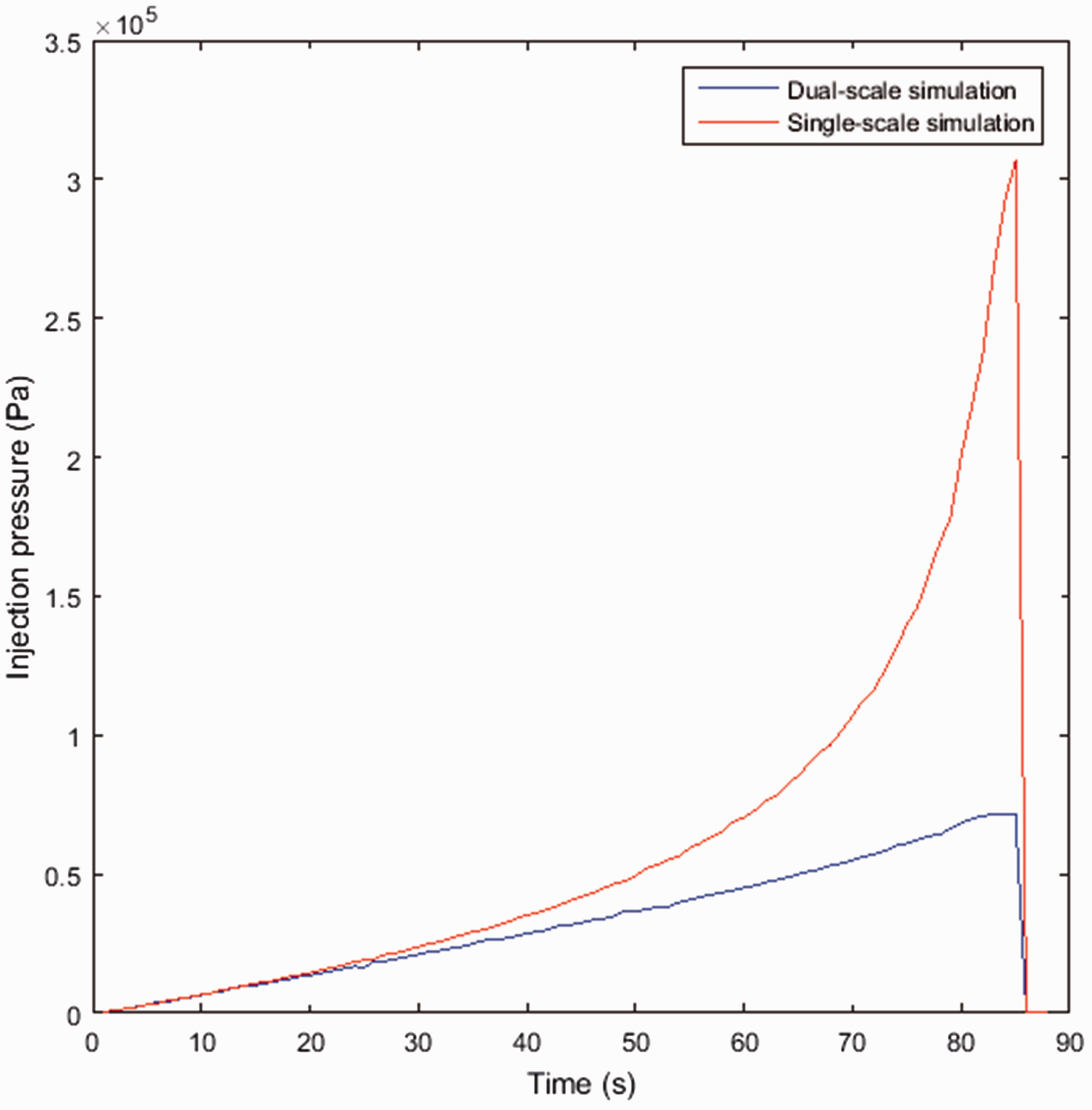
Injection pressures versus time obtained from the single and dual-scale reactive simulations.

In Figure 9, the values of temperature, degree of cure and viscosity referred as tows properties are the volume averaged values of theses quantities over the longitudinal elements of the microstructure containing fluid. Concerning fluid fraction, the mapped values are volume averaged over all longitudinal elements.

Fluid fraction

Figure 9 presents the mapping of the fluid fraction after 84 s of injection. It can be noticed that the predictions of the single-scale simulation state that the part is fully filled with the resin. However, in the dual-scale simulation, it can be observed that the tows are not saturated at the end of the cavity. This result highlights the fact that filling times predicted using single-scale approaches are incorrect to ensure the total channel and intra-tow saturation next to the vents for dual-scale porous materials.

Temperature

The temperature fields determined by single and dual-scale simulations may also be compared. One major difference can be noticed: the temperature of the part is higher close to the end of the cavity in the dual-scale simulation. In the dual-scale simulation, the resin flowing in the channels is indeed heated up all along its flowing to the end of the cavity by the tows where polymerization occurs. Thus the resin arrives hotter at the end of the cavity than in a single-scale simulation in which the resin has always been surrounded by resin with the same age.

Degree of cure

A major difference can be observed in the mapping of the degree of cure between the single and the dual-scale simulations. It is due to the resin storage in the tows. Indeed, in single-scale flows, as demonstrated experimentally in the literature, the oldest, most cured resin is located at the flow front. However, in dual-scale flows, the oldest resin is stored in the tows next to the injection point. This repartition can be observed very well in Figure 9. In the single-scale simulation, the degree of cure reaches 0.25 at the end of the cavity, while in the channels of the dual-scale simulation, the degree of cure is barely 0.2. In fact, the resin has been all along the filling removed from the flow front to be stored in the tows in the unsaturated area and replaced in the channels by younger less cured resin coming from the injection line.

Viscosity

As highlighted in equation (14) viscosity increases with increasing degree of cure and with decreasing temperature. As expected from the degree of cure and temperature mappings, the most viscous region in the part is located at the end of the cavity in the single-scale simulation compared to the dual-scale simulation. It can be thus noticed that the value of the viscosity in the channels in the dual-scale simulation is about six times smaller than the viscosity computed from the single-scale simulation. This has a significant influence on the injection pressure as can be observed in Figure 10. Furthermore, it can be noticed that the viscosity of the resin in the tows is higher than the viscosity in the channels. This is due to higher degree of cure of the resin in the tows while the temperatures of channel and tows are equivalent.

Pressure

It can be observed in Figure 10 that the injection pressure computed from the single-scale simulation evolves initially in the same way as the one computed from the dual-scale simulation. However, after about 25 s, it begins to increase faster until 84 s and the flow front arrival at the end of the cavity. This is due, as explained previously, to the higher increase in the resins viscosity at the flow front in the single-scale simulation. Furthermore, after 81 s, the pressure computed from the dual-scale simulation stops increasing. This moment corresponds to the arrival of the macroscopic flow front to the end of the cavity. This flow front arrival time is smaller than the one obtained from single-scale simulation as the volume to fill in the channels is smaller than the volumes of channels and tows combined. After 81 s, injection pressure is only affected by the evolution of the viscosity in the channels and the value of the sink term due to the fluid absorption in the tows. After 84 s, injection is stopped according to the injection time defined from the single-scale simulation. It can be finally observed from these curves that using a single-scale simulation instead of a dual-scale simulation may lead to a significant deviation in the prediction of the injection pressure.

The presented results highlight the fact that using single-scale simulation to define the optimum injection strategy for a reactive injection in a dual-scale textile may lead to mistakes in the prediction of the injection pressure so remaining unsaturated areas in the part next to the vents. Further simulations conducted with the developed dual-scale model may allow determining appropriate injection conditions to ensure part filling and reduce the overall processing time.

Conclusion

In this work, a new numerical strategy has been proposed to simulate in an efficient way the flow of a reactive resin in a dual-scale porous material. A pre-calculation step consists in associating to each element of the mesh, an equivalent microstructure. This microstructure is determined from the textiles characteristics and the size and shape of each element using purely geometric considerations. The microscopic filling problem can thus be reduced to one or two tow filling problems, depending on the type of textile considered (unidirectional or biaxial). The volume to be filled in the cavity is through this pre-calculation step spread between the macroscopic (channel) level and the microscopic (tow) level. A VOF technique inspired from Abisset-Chavanne and Chinesta⁵ is then used to deal both with the filling and reactive aspects of the simulation at the macroscopic scale. At the microscopic scale, a newly developed approach, based on a fixed transverse and adjustable longitudinal meshing of the tows is used to deal with the filling aspects and the VOF method allows tracking the quantities of interest (temperature, degree of cure). In the case of the studied high speed injections, adjustable longitudinal meshing of the tows allows reducing the tow filling problem to a sum of 1D transverse filling problems and to use macroscopic elements smaller or larger than the unsaturated area. These features make the approach more efficient in terms of calculation time and more flexible in terms of meshing.

Numerical simulations have been conducted to highlight the flexibility of the method. It has been demonstrated on a simple dual-scale 1D filling simulation that increasing the size of the elements by a factor 10 only led to small errors (smaller than 6%) on the injected fluid over time. In this case, the elements used were more than three times bigger than the unsaturated area and the computation time less than 1/100 of the computation time with the refined mesh. Furthermore, single and dual-scale simulations of a reactive injection have been compared and the necessity of using a dual-scale simulation to ensure an appropriate tracking of the quantities of interest and thus a full filling of the part has been demonstrated.

Finally, the developed approach has demonstrated to show interesting ability to deal with dual-scale injection cases with on-line mixing. It must be however emphasized that, due to the assumption of purely transverse tow saturation, the developed method is only valid for high speed flow regimes. Future numerical work will be therefore needed to extend the presented techniques to flow regimes where capillary effects induce non-negligible intra-tow longitudinal flow velocity compared to the channel flow velocity. Furthermore, experimental work should be conducted in order to validate the assumptions made and confirm the effects of dual-scale flow highlighted by the simulations.

Footnotes

Declaration of Conflicting Interests

The author(s) declared no potential conflicts of interest with respect to the research, authorship, and/or publication of this article.

Funding

The author(s) disclosed receipt of the following financial support for the research, authorship, and/or publication of this article: Part of the funding was provided by the French ANRT grants under CIFRE funding program.

References

Roy T, Dulmes C and Pillai K. Experimental investigations of the unsaturated flow in liquid composite molding. In: 5th Canadian International Composites Conference, Vancouver, 2005.

Bruschke

Advani

. Finite element/control volume approach to mold filling in anisotropic porous media. Polym Compos 1990; 11: 398–405.

Trochu

Gauvin

Gao

D-M

. Numerical analysis of the resin transfer molding process by the finite element method. Adv Polym Technol 1993; 12: 329–342.

Deléglise

Grognec

Binetruy

et al.

Modeling of high speed RTM injection with highly reactive resin with on-line mixing. Compos A: Appl Sci Manufact 2011; 42: 1390–1397.

Abisset-Chavanne

Chinesta

. Toward an optimisation of the reactive resin transfer molding process: thermo-chemico-mechanical coupled simulations. Int J Mater Forming 2013; 7: 249–258.

Tan

Pillai

. Multiscale modeling of unsaturated flow of dual-scale fiber preform in liquid composite molding III: reactive flows. Compos A: Appl Sci Manufact 2012; 43: 29–44.

Simacek

Advani

. A numerical model to predict fiber tow saturation during liquid composite molding. Compos Sci Technol 2003; 63: 1725–1736.

Wang

Anderson

. Introduction to groundwater modeling: finite difference and finite element methods, San Diego: Academic Press, 1982.

Tan

Pillai

. Multiscale modeling of unsaturated flow in dual-scale fiber preforms of liquid composite molding I: isothermal flows. Compos A: Appl Sci Manufact 2010; 43: 1–13.

10.

Sanchez

Garcia

Gascon

et al.

Towards an efficient numerical treatment of the transport problems in the resin transfer molding simulation. Comput Methods Appl Mech Eng 2007; 196: 2300–2312.

11.

Tan

Pillai

. Numerical simulation of reactive flow in liquid composite molding using flux-corrected transport (FCT) based finite element/control volume (FE/CV) method. Int J Heat Mass Transf 2010; 53: 2256–2271.

12.

Darcy H. Les Fontaines Publiques de la Ville de Dijon: Exposition et Application, Victor Dalmont, 1856.

13.

Pillai

Advani

. Numerical simulation of unsaturated flow in woven fiber preforms during the resin transfer molding process. Polym Compos 1998; 19: 71–80.

14.

M-K

Lee

. A study on the mold filling process in resin transfer molding. Polym Eng Sci 1991; 31: 765–771.

15.

Wang

Grove

. Modelling microscopic flow in woven fabric reinforcements and its application in dual-scale resin infusion modelling. Compos A: Appl Sci Manufact 2008; 39: 843–855.

16.

Kelly

Umer

Bickerton

. Viscoelsatic responce of dry and wet fibrous materials during infusion processes. Compos A: Appl Sci Manufact 2006; 37: 868–873.

17.

Pillai

Jadhav

. A numerical study of nonisothermal reactive flow in a dual-scale porous medium under partial saturation. Numer Heat Transfer A: Appl Int J Comput Methodol 2007; 47: 109–136.

18.

Gebart

. Permeability of unidirectional reinforcements for RTM. J Compos Mater 1992; 26: 1100–1133.

19.

Schell

Deleglise

Binetruy

et al.

Numerical prediction and experiemental characterisation of meso-scale voids in liquid composite moulding. Compos A: Appl Sci Manufact 2007; 38: 2460–2470.

20.

Ivankovic

Incarnato

Kenny

LNJM

. Curing kinetics and chemorheology of epoxy anhydride system. J Appl Polym Sci 2003; 90: 3012–3019.

21.

Ahn

Seferis

JBJC

. Simultaneous measurements of permeability and capillary pressure of thermosetting matrices in woven fabric reinforcements. Polym Compos 1991; 12: 146–152.