Strain rate-dependent large deformation inelastic behavior of an epoxy resin

Abstract

The objective of this paper is to model high strain rate and temperature-dependent response of an epoxy resin (DER 353 and bis(p-aminocyclohexyl) methane (PACM-20)) undergoing large inelastic strains under uniaxial compression. The model is decomposed into two regimes defined by the rate and temperature-dependent yield stress. Prior to yield, the model accounts for viscoelastic behavior. Post yield inelastic response incorporates the effects of strain rate and temperature including thermal softening caused by internal heat generation. The yield stress is dependent on both temperature and strain rate and is described by the Ree–Erying equation. Key experiments over the strain rate range of 0.001–12,000/s are conducted using an Instron testing machine and a split Hopkinson pressure bar. The effects of temperature (25–120 ℃) on yield stress are studied at low strain rates (0.001–0.1/s). Stress-relaxation tests are also carried out under various applied strain rates and temperatures to obtain characteristic relaxation time and equilibrium stress. The model is in excellent agreement over a wide range of strain rates and temperatures including temperature in the range of the glass transition. Case studies for a wide range of monotonic and varying strain rates and large strains are included to illustrate the capabilities of the model.

Keywords

Epoxy resin Ree–Eyring model stress relaxation temperature effects

Introduction

Epoxy resins, one of the most commonly used thermoset polymers, are extensively used in military and structural composite applications due to their highly crosslinked molecular structure which results in superior mechanical properties (modulus and strength) and thermal stability compared to other matrices.¹ Under impact, shock, or ballistic loading, fiber-reinforced polymer composite structures can be highly sensitive to strain rate and temperature that originates from the response of polymer matrix subjected to high levels of compression deformation at high strain rate.^2–4 Various experimental methods are often used in conjunction with finite element modeling of microstructure to gain a better understanding of matrix deformation and failure mechanisms involved in polymer composites subjected to various loading scenarios.^5,6

For example, during an event of tensile failure in the fiber direction in S-glass fiber-reinforced epoxy composites, failure initiates in the form of a dynamic fiber breaks due to relatively lower strain to failure of fibers.⁷ Once a critical number of fiber breaks locally cluster together, the composite fails catastrophically. Such behavior makes it extremely important to understand the localized strain rate-dependent deformation and damage mechanisms, such as matrix yielding, microcracking, and interfacial debonding that accompanies fiber breaks, in order to accurately predict the failure of these composites.^8,9 Fiber breakage within a composite is a highly dynamic process even when the applied loading rate in the composite is in quasi-static range.^9–11 When a fiber breaks, stress wave propagation occurs due to the dynamic release of stored elastic energy in the fiber and the local strain rates in the matrix approaches 10⁵–10⁶/s and then rapidly drops to the far-field applied strain rate (∼10⁻³/s) as the dynamic effects subside. This event occurs within an extremely short time-span of around 50 ns in glass-epoxy composites.¹⁰ Moreover, since the matrix is locally subjected to large plastic strains at high rates, adiabatic heating and thermal softening are likely to occur in the vicinity of fiber breakage. The matrix response at the fiber break has also been shown to significantly affect initiation and propagation of interface debonding.^12–15 In order to accurately capture the progression of damage accompanying a fiber break using micromechanical FE models, there is a need to formulate a temperature and strain rate-dependent model for the epoxy matrix spanning from 10⁻³ to 10⁶/s that can handle abrupt increases in strain rate, high levels of plasticity, and adiabatic heating/thermal softening effects due to fiber breaks followed by rapid loading/unloading and stress relaxation.

General constitutive behavior of glassy polymer under monotonic loading consists of initial increase in stress–strain up to yield followed by post yield softening and strain hardening at large strain. For the prediction of the initial stress–strain response of polymers, significant contribution has been made by Mahieux and Reifsnider¹⁶ in developing a temperature-dependent stiffness model, which was later modified by Richeton et al.¹⁷ to include strain-rate dependency. Other researchers^18–20 have used viscoelastic models using different combinations of spring and dashpot to predict the non-linear stress–strain behavior up to yield when subjected to monotonic loading.

In amorphous glassy polymers, pure viscous flow takes place momentarily during yielding, and this process is dependent on applied strain rate and temperature.^21,22 Eyring-type equation is commonly used to predict strain rate and temperature-dependent yield stress, which is treated as a thermally activated process.^23,24 The molecular segmental mobility during yielding has been proposed to be analogous to the mobility during glass transition, suggesting that the applied stress essentially reduces the T_g of the material to the test temperature until yielding occurs.²⁵ Roetling^22,26 proposed that more than one type of molecular segmental motion (α and β relaxation) is involved, and the total stress is the sum of stresses carried out by various processes. Mulliken and Boyce²⁷ adopted a similar approach to capture the transition in yield behavior which is manifested by bilinear relation of yield stress with strain rate when plotted on a log scale. They also developed physically based constitutive model consisting of spring and dashpot with α and β components to describe hardening at large strains. Richeton et al.²⁸ extended the capability of Eyring model to predict the yield stress beyond glass transition temperature by correlating the yield behavior to the secondary relaxation.

Post yield softening behavior has been described analytically by several researchers using damage models. Nemes and Spéciel²⁹ developed a continuum damage model to describe rate-dependent response of composite laminates under dynamic loading. Frantziskonis and Desai³⁰ modeled strain softening by treating it as a result of non-homogeneity in the deformation and stress fields. Van Breemen et al.³¹ modified elasto-viscoplastic Eindhoven glassy polymer model to incorporate strain rate and temperature-dependent strain softening in solid polymers.

Strain hardening has been linked to network density (via chemical crosslinking or network entanglement), molecular chain reorientation, and alignment.^25,32–35 Mechanisms behind strain rate and temperature dependence of strain hardening is different from yielding.³³ Arruda et al.³⁶ modeled strain hardening by decomposing inelastic deformation into non-dissipative internal back stress component and the remaining dissipative plastic work contributing to heat generation. Pan et al.³⁷ determined inelastic heat fraction and used multiplicative factors to incorporate thermal softening at high strain rate in their constitutive model. While modeling the hardening behavior, especially at high rates of loading, it is important to consider thermal softening due to adiabatic softening as strain rate and thermal effects are often coupled.

Polymeric materials are also known to exhibit stress relaxation when the displacement is held constant after being subjected to a certain strain rate, where the material relaxes toward an equilibrium state. Time-dependent standard viscoelastic spring and dashpot models work well in describing the relaxation process in polymers.^18,19 Bergstrom³⁸ modeled this behavior by using two networks in parallel—one captures the equilibrium state and the other predicts the time-dependent deviation from the equilibrium, which is based on reptational motion of molecules.

In our previous work,³⁹ compressive properties of epoxy resin DER 353 were experimentally characterized under high strain rate over large strains at a wide range of temperatures. DER 353 is an epoxy manufactured by Dow Chemical Company and is mixed with PACM-20 curing agent (Air Products and Chemicals, Inc.) at stoichiometric ratio of 100:28 (weight ratio). The mixture was allowed to gel at room temperature for 5 h, followed by curing at 80 and 150 ℃ for 2 h each. Hopkinson bar (10³–10⁴/s strain rate) tests on the epoxy resin exhibited thermal softening resulting in complete absence of hardening at large strain, which led to the experimental investigation on temperature effects. Effect of temperature on stress–strain response at lower strain rates was also studied. Also, stress-relaxation tests at different loading rates are conducted in the current study to determine the model parameters. In this paper, an algorithm based on an incremental approach to predict full stress–strain response is developed, which includes estimation of rise in specimen temperature to predict thermal softening. Finally, model predictions for different loading/unloading scenarios, strain-rate jumps, and stress relaxation are presented.

Development of large deformation inelastic model for dynamic behavior

In this study, a model is developed that is experimentally validated over a wide range of strain rates (from 10⁻³−10⁴/s) and temperatures (from ambient to above T_g) including thermal softening at high strain rates. As such, this model considers the change in the state of the polymer from glassy to rubber-like behavior as the temperature of the material rises above T_g. The model can also handle abrupt changes in loading rates, including zero strain rate, i.e. stress relaxation.

The algorithm developed for the description of material behavior is depicted in the flowchart presented in Figure 1. Strain–time profile and the initial temperature of the material serve as inputs for the initiation of calculations. At each incremental time step, strain rate, stress, and temperature are calculated and updated to be used for the subsequent increments. The first step is to categorize if the material is being loaded or unloaded, or if the deformation is held constant (stress relaxation). If the strain rate is negative, stress value is reduced at a slope of the modulus based on the unloading strain rate and current temperature. If the strain rate is zero, relaxation occurs, and the reduction in stress value is calculated based on the previously known positive strain rate, current temperature, and strain level. For positive strain rates, it should be determined whether the material has yielded. Then, relevant equations are applied for the calculation of stress depending on whether the material is in elastic or plastic state. For high rate of loading, thermal softening has been incorporated through the estimation of heat generation due to plastic work.

Figure 1.

Flowchart showing the algorithm for time and temperature-dependent model with incremental approach.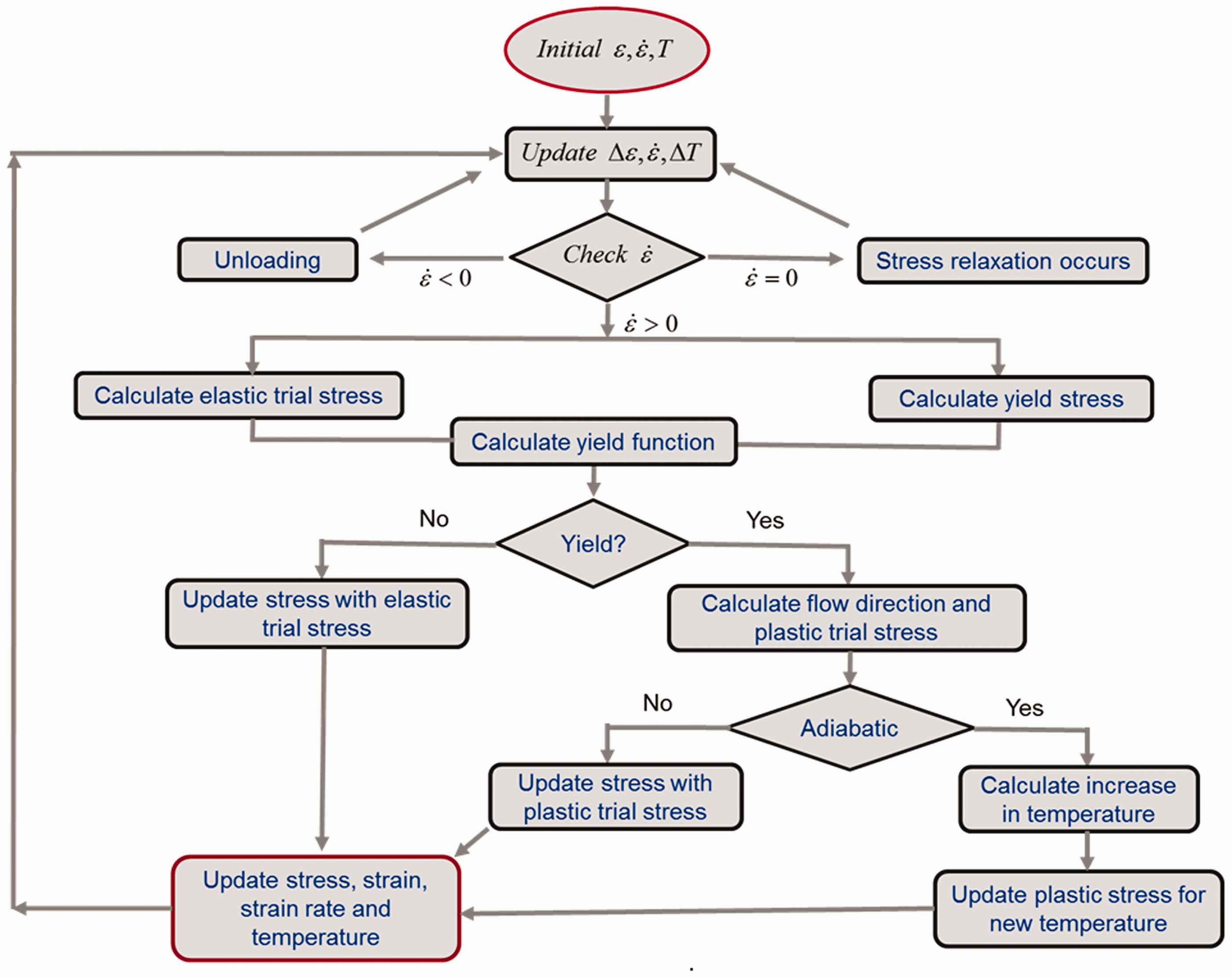

Decomposition of stress–strain response

A typical stress–strain response of DER 353 resin subjected to monotonic loading exhibits initial increase in stress until yield followed by post yield softening, plastic flow, and finally strain hardening at large strains (Figure 2). The model decomposes the stress–strain response into pre-yield (elastic or viscoelastic) and post-yield (strain rate and temperature-dependent plastic) regimes based on the yield stress, which is defined as a point $(d σ / d ɛ = 0)$ , where pure viscous flow takes place momentarily (Figure 2). Stress–strain response up to yield as a function of strain rate and temperature is described using a spring and dashpot model. Eyring-type equation is used to predict strain rate and temperature-dependent yield stress. For the prediction of post-yield behavior, the plastic flow obtained at different temperatures is used.

Figure 2.

Stress–strain curve is decomposed into elastic and plastic regime. Three different sets of equations are used to model elastic and plastic portion of the curve and yield stress.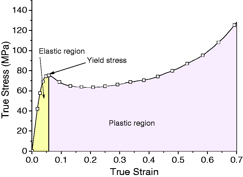

Determination of yield function

Accurate determination of yield stress and strain is very crucial in the development of this model as it links the elastic and plastic portion of the curve. For each incremental step, it needs to be determined whether the material is in elastic or plastic state for the given strain rate and temperature. First, yield stress is calculated using Ree–Eyring equation, and elastic trial stress is calculated using viscoelastic model for the given condition ( $\overset{\cdot}{ɛ} & T)$ . If the elastic trial stress is less than the yield stress, then the material is still in elastic region, and the stress value is updated with the elastic trial stress. However, if the elastic trial stress is greater than the yield stress, the material has yielded, and the yield strain is calculated. Subsequently, plastic strain is determined, and the elastic trial stress is replaced by plastic trial stress.

Determination of model parameters

In this section, experimental work for the determination of strain rate and temperature-dependent stress–strain response and stress-relaxation behavior is presented. The experimental results are then used to determine the model parameters.

Stress–strain response for monotonic loading (strain rate > 0)

Experimental determination of strain rate-dependent properties

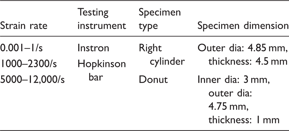
Strain rate-dependent properties of DER 353 epoxy resin were determined using Instron testing machine for lower rates and split Hopkinson pressure bar for higher rates. Aluminum 6061 was used for incident, transmission, and striker bar, which were precision machined and centerless ground. Specimen type and dimensions used for different rates are presented in Table 1. Specimen failure occurred within the first loading pulse. More details regarding experimental setup and specimen design are presented in our previous work.³⁹

Table 1.

Specimen type and dimensions for different strain rates.

Strain rate	Testing instrument	Specimen type	Specimen dimension
0.001–1/s	Instron	Right cylinder	Outer dia: 4.85 mm, thickness: 4.5 mm
1000–2300/s	Hopkinson bar	Right cylinder	Outer dia: 4.85 mm, thickness: 4.5 mm
5000–12,000/s	Hopkinson bar	Donut	Inner dia: 3 mm, outer dia: 4.75 mm, thickness: 1 mm

True stress–strain response for strain rates 0.001–1/s is presented in Figure 3(a). The overall trend of the stress–strain response is similar for all four strain rates—initial increase in stress is observed until the yield point is reached, which is followed by strain softening and plastic flow. The initial slope of the stress–strain curve slightly increases with strain rate. There is a significant effect of strain rate on the yield stress, which increases from 85 MPa at 0.001/s to 220 MPa at 12,000/s strain rate.

Figure 3.

Stress–strain response of DER 353 resin at strain rates of (a) 0.001–1/s shows typical post yield softening and strain hardening and (b) 1000–12,000/s shows thermal softening at large strain due to adiabatic heating.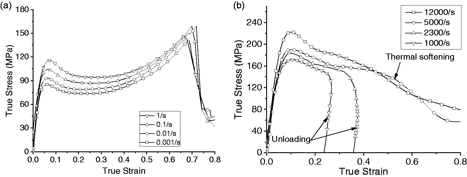

In high strain rate tests, it is very challenging to maintain a uniform strain along the length of the specimen during the test. One way to reduce the spatial variability of strain and strain rate in the specimen is to reduce the length of the specimen. However, the reduction in length can contribute to a high aspect ratio (L/D) leading to increased frictional stresses. This issue was resolved by drilling a hole at the center of the specimen. Finite element analysis of donut specimens shows that the state of stress remains uniform throughout the specimen, and the frictional effects are minimized. The presence of the hole at the center also minimizes inertial stresses induced in the radial direction.

At higher strain rates, specimen gets less time to dissipate the heat generated due to plastic work, resulting in rise in specimen temperature (i.e. adiabatic heating). Thermal softening at high strain rates (5000/s and 12000/s) results in complete absence of strain hardening at large strains (Figure 3(b)). Estimation of specimen temperature assuming complete conversion of plastic work into heat energy shows that the resin enters glass transition temperature at around 45–50% strain level and becomes completely rubbery when it reaches 70% strain.³⁹

Experimental determination of temperature-dependent properties

Thermal softening of high ductility polymeric materials due to adiabatic heating at high strain rate is inevitable, especially for materials with low T_g. Temperature-dependent response of the material needs to be considered to develop a comprehensive model. Dynamic mechanical analysis was carried out using Mettler DMA 861 for the determination of T_g. Experiments were conducted on right cylinder specimens (6 mm diameter and 1.8 mm thick) in shear mode at 1 Hz frequency over a temperature range of 25–180 ℃ while maintaining a constant shear stress of 1.77 kPa. When considering the mechanical aspect of a material, T_g based on storage modulus is used in general. Figure 4(a) shows the T_g range, the beginning of which is marked by an abrupt change in the storage modulus at around 70 ℃, spans to about 100 ℃.

Figure 4.

(a) Temperature-dependent stress–strain response under isothermal condition at 0.001/s strain rate and (b) stress–strain response at 100 ℃ shows transition from rubbery behavior at 0.001/s to typical glassy behavior at 0.1/s strain rate.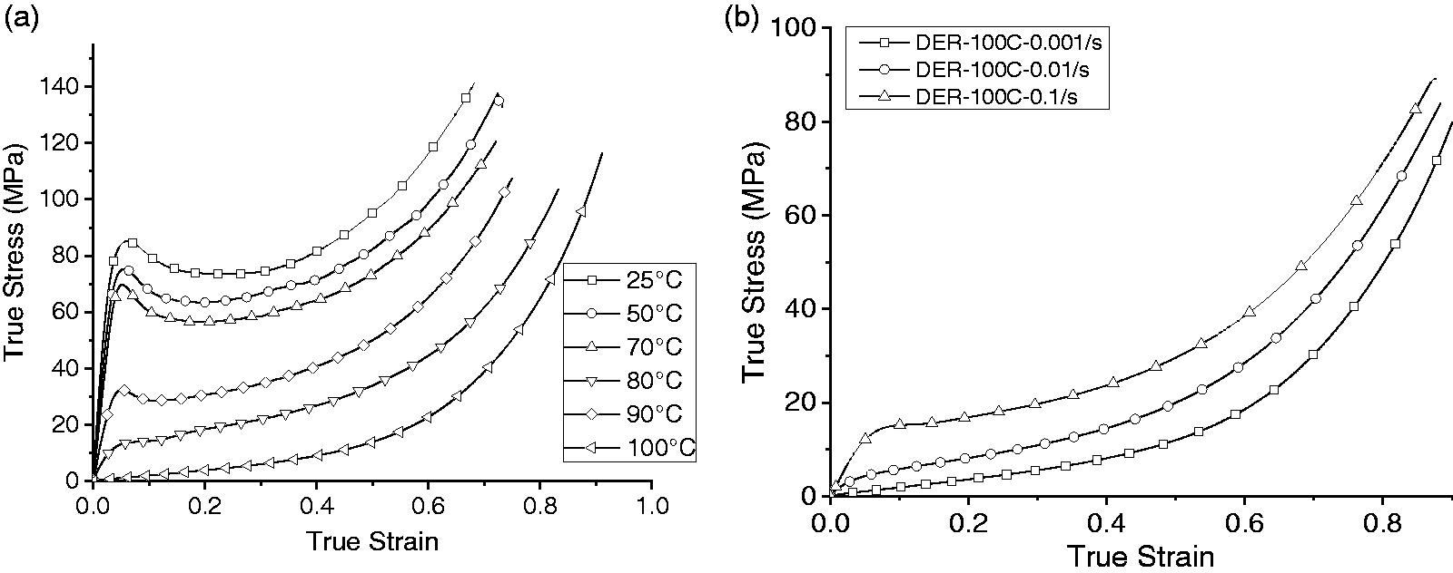

To obtain full stress–strain response from ambient temperature to above T_g range, quasi-static tests were conducted at a strain rate of 0.001–0.1/s on right cylinder specimen under isothermal conditions at 25, 50, 70, 80, 90, 100, 110, 120, and 150 ℃. Figure 4(b) shows that yield stress, modulus, and compressive strength are significantly affected by temperature. Detailed explanation on the experimental results are presented in our previous paper.³⁹ The following key observations were made on the compressive stress–strain behavior of the epoxy resin when the test temperature was increased from ambient to 150 ℃:

Up to T_g (ambient to 70 ℃);

° Initial non-linear increase in stress followed by a distinct yield point;

° Typical glassy polymer behavior showing post yield softening, plastic flow, and strain hardening;

° Same shape of the plastic portion of the curve for all temperatures:

• T_g range (70–100 ℃);

° Yield stress significantly reduces above T_g;

° Post yield softening start to vanish at 80 ℃, exhibiting more rubbery behavior;

° Strain hardening is still present and is similar to ones at lower temperatures;

° At 100 ℃, there is no definite yield point $(d σ / d ɛ = 0)$ , and the material behaves more like an elastomer exhibiting strain hardening;

° At 100 ℃, rubbery elastic epoxy at 0.001/s showed typical glassy behavior at 0.1/s with a distinct yield point:

• Above T_g (100–150 ℃);

° When tested at 0.001/s strain rate, the epoxy exhibited pure elastic rubbery behavior;

° Stress–strain behavior at 0.001/s above 120 ℃ up to 150 ℃ was found to be identical;

° As the temperature was increased further above T_g, the epoxy resin became less sensitive to strain rate.

These observations have provided guidance on our approach to model the material response in each temperature range.

Prediction of stress strain response up to yield point

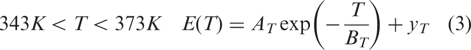
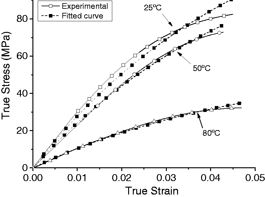
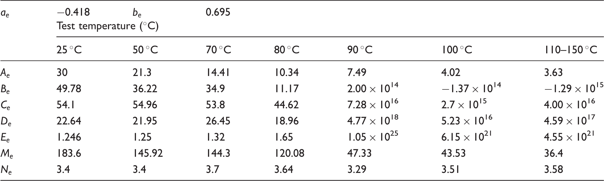
Analytical solution for a viscoelastic standard linear solid model subjected to monotonic loading (equation (1)) has been calibrated using experimental results to predict the stress–strain response up to yield as a function of temperature and strain rate. Equations (2) and (3) predict the temperature-dependent elastic modulus of the spring. Strain-rate effects have been incorporated in the model by using a scaling factor, $r (\overset{\cdot}{ɛ})$ which is based on strain-rate dependency of the elastic modulus of the material (equation (4)). Fitting parameters are presented in Table 2. A comparison of experimental and model prediction of stress strain response subjected to 0.001/s strain rate at different temperatures is presented in Figure 5

\begin{matrix} 0 < σ < σ_{y} \\ σ_{e} (ɛ, \overset{\cdot}{ɛ}, T) = τ \cdot E (T) \cdot r (\overset{\cdot}{ɛ}) \cdot \overset{\cdot}{ɛ} \cdot (1 - exp (- \frac{ɛ}{τ \overset{\cdot}{ɛ}})) \end{matrix}

(1)

T \leq 343 K E (T) = m_{T} T + c_{T}

(2)

\begin{matrix} 343 K < T < 373 K E (T) = A_{T} exp (- \frac{T}{B_{T}}) + y_{T} \end{matrix}

(3)

\begin{matrix} r (\overset{\cdot}{ɛ}) = a_{SR} + b_{S R} {\overset{\cdot}{ɛ}}^{c_{SR}} \end{matrix}

(4)

Figure 5.

Goodness of fit plots for the pre-yield portion of the stress strain curve at different temperatures (strain rate: 0.001/s).

Table 2.

Curve-fitting parameters.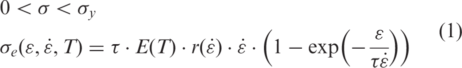

τ(s)	50
$m_{T}$ (MPa/K)	7750.7
$c_{T}$ (MPa)	−15.73
$A_{T}$ (MPa)	4.88 × 10¹¹
$B_{T}$	18.1
$y_{T}$ (MPa)	−494
$a_{SR}$	1.083
$b_{SR}$	0.043
$c_{SR}$	0.299

Prediction of yield stress

Yield stress varies bi-linearly as a function of strain rate when plotted on a semi-log scale (Figure 6(a)), suggesting that more than one type of molecular segmental motions is involved at higher strain rates.²² Alpha relaxation, which is associated with rotational freedom in the segments between crosslinks, is involved at lower strain rates. Whereas, at higher strain rates, since there is less time for the polymer chains to reorient and slide, side chain motion also gets activated resulting in beta relaxation,³ which occurs at about 100/s strain rate for 25 ℃ test temperature for the epoxy resin DER 353 considered in this study.

Figure 6.

(a) Yield stress shows bilinear relation with strain rate when plotted on a semi-log scale. Yielding at high strain rates is comprised of both α and β-relaxation and (b) strain rate and temperature-dependent yield stress predictions using Ree–Eyring model.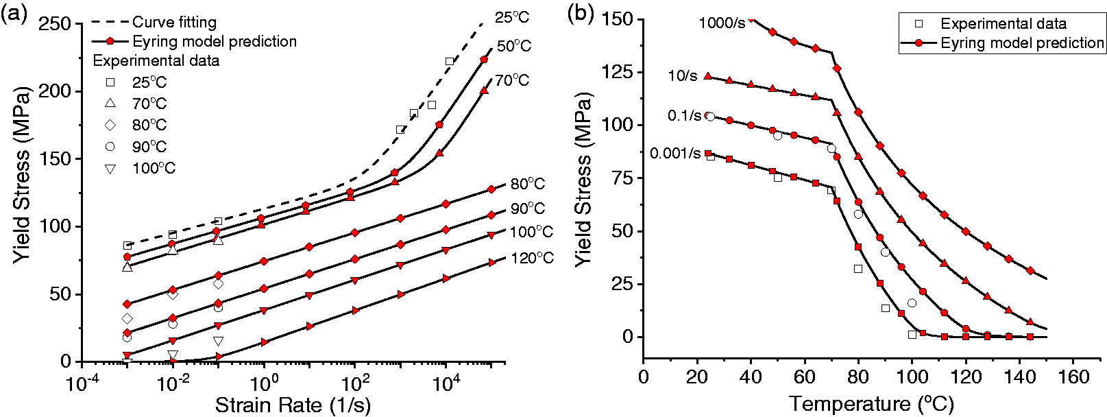

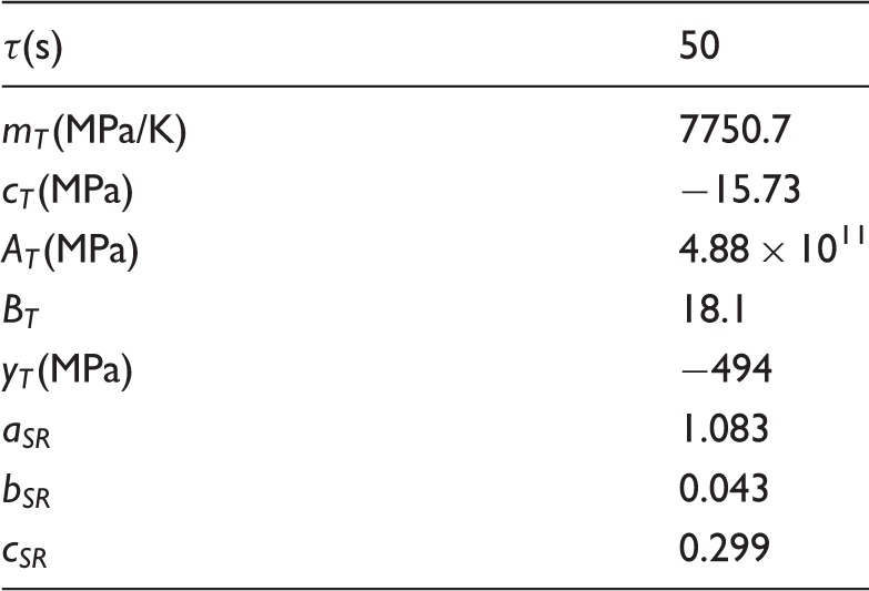
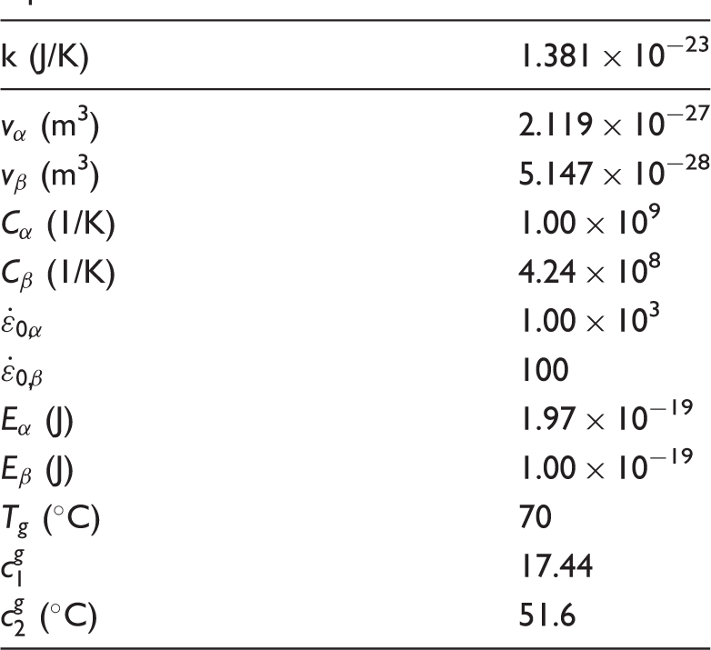
Yield stress as a function of strain rate and temperature is modeled using Ree–Eyring equation.^25,26 For the determination of the Ree–Eyring model parameters (equation (5)), the yield stress versus strain-rate curves are decomposed into alpha and beta-relaxation processes. The model parameters activation volumes (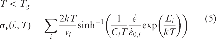 $v_{α}$ and $v_{β}$ ), activation energies ( $E_{α}$ and $E_{β}$ ), pre-exponential factors ( ${\overset{\cdot}{ɛ}}_{0, α}$ and ${\overset{\cdot}{ɛ}}_{0, β}$ ), and model constant ( $C_{α}$ and $C_{β}$ ) are then determined for the particular process (α and β contribution). For the prediction of the yield stress above T_g, WLF equation is incorporated in the Ree–Eyring equation (equation (6)) as proposed by Richeton et al.²⁸ For glass transition parameter, T_g in equation (6), a single temperature (70 ℃) corresponding to the initial point in the transition range is used despite the fact that T_g occurs over a range of temperature.

\begin{matrix} T < T_{g} \\ σ_{y} (\overset{\cdot}{ɛ}, T) = \sum_{i} \frac{2 kT}{v_{i}} \sinh^{- 1} (\frac{1}{C_{i} T} \frac{\overset{\cdot}{ɛ}}{{\overset{\cdot}{ɛ}}_{0, i}} exp (\frac{E_{i}}{kT})) \end{matrix}

(5)

\begin{matrix} \begin{matrix} \begin{matrix} T \geq T_{g} \\ i = α, β \end{matrix} & σ_{y} (\overset{\cdot}{ɛ}, T) = \sum_{i} \frac{2 kT}{v_{i}} \sinh^{- 1} \end{matrix} \\ (\frac{1}{C_{i} T} \frac{\overset{\cdot}{ɛ}}{{\overset{\cdot}{ɛ}}_{0, i}} \frac{exp (\frac{E_{i}}{kT})}{exp (\frac{\ln (10) \cdot c_{1}^{g} (T - T_{g})}{c_{2}^{g} + T - T_{g}})}) \end{matrix}

(6)

Model parameters presented in Table 3 were obtained using yield stresses experimentally obtained for test temperature of 25 ℃ over strain rates of 0.001–12,000/s, and then predictions were made for higher temperatures. Independent experiments at higher temperatures (50, 70, 80, and 90 ℃) at strain rates of 0.001, 0.01, and 0.1/s were carried out to validate the Ree–Eyring model predictions. Percentage error in the model predictions is presented in Table 4. Model prediction shows excellent correlation with the experiments up to 70 ℃ with an error below 5%. Although the accuracy of the model starts to diminish as the material enters T_g range, the accuracy of the model is still reasonable up to 90 ℃. Model prediction shows less rate sensitivity as the temperature is increased above T_g as evidenced by the experiments.

Table 3.

Model parameters for Ree–Eyring equation.

k (J/K)	1.381 × 10⁻²³
$v_{α}$ (m³)	2.119 × 10⁻²⁷
$v_{β}$ (m³)	5.147 × 10⁻²⁸
$C_{α}$ (1/K)	1.00 × 10⁹
$C_{β}$ (1/K)	4.24 × 10⁸
${\overset{\cdot}{ɛ}}_{0, α}$	1.00 × 10³
${\overset{\cdot}{ɛ}}_{0, β}$	100
$E_{α}$ (J)	1.97 × 10⁻¹⁹
$E_{β}$ (J)	1.00 × 10⁻¹⁹
$T_{g}$ (℃)	70
$c_{1}^{g}$	17.44
$c_{2}^{g}$ (℃)	51.6

Table 4.

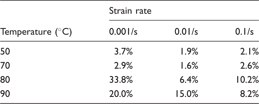
Percentage error in Ree–Eyring model prediction.

	Strain rate
Temperature (℃)	0.001/s	0.01/s	0.1/s
50	3.7%	1.9%	2.1%
70	2.9%	1.6%	2.6%
80	33.8%	6.4%	10.2%
90	20.0%	15.0%	8.2%

As expected, model prediction shows increased yield stress as the temperature is decreased. The validity of the model at lower strain rate can be checked using the yield stress obtained from the equilibrium tests. The equilibrium yield stress corresponds to zero strain rate, which means that the yield stress cannot fall below this value. For 25 ℃, equilibrium yield stress is about 71 MPa. This value corresponds to Ree–Eyring prediction for strain rate of 10⁻⁵/s, which can be considered as the lower limit for strain-rate prediction. As for the upper limit for the strain rates, predictions made by molecular dynamics simulation for similar epoxy show a yield stress of about 300 MPa when subjected to a strain rate of 10⁹/s.⁴⁰ This value can be considered a theoretical maximum. Ree–Eyring model predicts a yield stress of this value at a strain rate of 10⁶/s. Therefore, this strain rate can be marked as the upper limit on model's predictive capability.

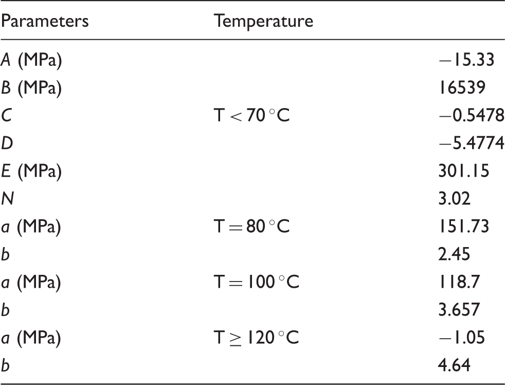
Prediction of post yield plastic response

Temperature-dependent post yield response of the epoxy is predicted by first describing the shape of the curve (equations (7) and (9)) and then adding the corresponding yield stress predicted by Ree–Eyring model (equation (10)). As mentioned earlier, the initial post yield softening portion, observed at lower temperature under isothermal condition at quasi-static loading condition, becomes less prominent as the material approaches T_g range (Figure 4(b)). The shape of the post yield curves for 25 to 70 ℃ is essentially the same and is modeled using equation (7). The behavior then transitions to almost no post yield softening at 80 ℃, which is described using equation (8). Fitting parameters for equations (7) and (8) are presented in Table 5. To avoid overlapping of the stress−strain curves during prediction between 70 and 80 ℃, the stress values are linearly interpolated for a given strain between equations (7) and (8). The material becomes completely rubbery at and above 100 ℃ as evidenced by the DMA results (Figure 4(a)). Prediction of stress–strain response between 80 and 120 ℃ is done by linearly interpolating the stress values for a given strain as mentioned before

\begin{matrix} 25^{\circ} C < T < 70^{\circ} C \\ σ_{shp} (ɛ_{p}) = A + \frac{B}{1 + 10^{(C - ɛ_{p}) D}} + E ɛ_{p}^{N} \end{matrix}

(7)

80^{\circ} C < T < 120^{\circ} C σ_{shp} (ɛ_{p}) = a ɛ_{p}^{b}

(8)

T \geq 120^{\circ} C σ_{shp} (ɛ_{p}) = a (1 - e^{b ɛ_{p}})

(9)

σ_{p} (ɛ, \overset{\cdot}{ɛ}, T) = σ_{y} (\overset{\cdot}{ɛ}, T) + σ_{shp} (ɛ_{p})

(10)

Table 5.

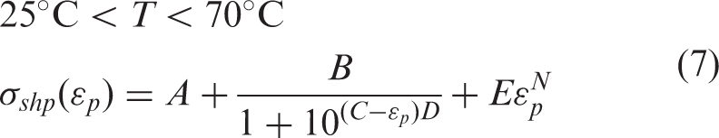
Curve-fitting parameters.

Parameters	Temperature
A (MPa)		−15.33
B (MPa)		16539
C	T < 70 ℃	−0.5478
D		−5.4774
E (MPa)		301.15
N		3.02
a (MPa)	T = 80 ℃	151.73
b	T = 80 ℃	2.45
a (MPa)	T = 100 ℃	118.7
b	T = 100 ℃	3.657
a (MPa)	T ≥ 120 ℃	−1.05
b	T ≥ 120 ℃	4.64

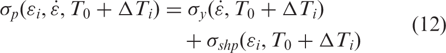
Prediction of plastic stress with thermal softening

If adiabatic conditions exist, thermal softening is also taken into consideration by calculating the rise in material temperature using equation (11), assuming all the plastic work is converted to heat

Δ T_{i} = \frac{β}{ρ c} \int_{ɛ_{y}}^{ɛ_{i}} σ (ɛ, \overset{\cdot}{ɛ}) \cdot d ɛ

(11)

where β is inelastic heat fraction, ρ is density (1150 kg/m³), and c is specific heat capacity of the epoxy specimen (1.11 kJ/kg K). The inelastic heat fraction was estimated by determining the specimen temperature through the intersection of the experimental high rate curve exhibiting thermal softening and predicted isothermal curves for different temperatures at the given strain rate. Isothermal curves at higher strain rates were constructed by vertically shifting the quasi-static curves using yield stresses predicted by Ree–Eyring equation. Detailed procedure is outlined elsewhere.⁴¹ In cases where heat loss occurs, and adiabatic conditions do not exist, a coupled problem (deformation and heat transfer) must be solved to predict the time-dependent temperature in lieu of equation (11). Figure 7(a) shows an example for the calculation of stresses with thermal softening under adiabatic condition. The dotted line shows the predicted stress and the solid lines represent stress–strain response predicted using equations (7) to (9) under isothermal condition for strain rate of 5000/s at temperatures 25–100 ℃. It is not possible to simultaneously predict both stress and temperature for a new strain increment. Therefore, to predict the stress value with thermal softening for step i (in Figure 7(a)), a trial plastic stress

(σ_{p, trial})

is first calculated assuming no change in temperature from the previous step

(σ_{p, i - 1})

by following the shape of the isothermal curve for the given strain rate. The estimated rise in temperature due to plastic work during this strain increment is calculated. Then, finally, the plastic stress

(σ_{p, i})

is calculated based on the estimated rise in temperature of the material knowing the current strain rate. If the strain increment is kept small enough, the error in the calculation of plastic work is negligible and does not affect the prediction results (in this case, time steps corresponding to 0.1% strain increment were used). Figure 7(b) shows good agreement between the experimental result and model prediction of stress–strain response for DER 353 epoxy resin tested at ambient temperature under a strain rate of 5000/s including thermal softening due to adiabatic heating

\begin{matrix} σ_{p} (ɛ_{i}, \overset{\cdot}{ɛ}, T_{0} + Δ T_{i}) = σ_{y} (\overset{\cdot}{ɛ}, T_{0} + Δ T_{i}) \\ + σ_{shp} (ɛ_{i}, T_{0} + Δ T_{i}) \end{matrix}

(12)

Figure 7.

(a) Prediction of stress–strain response at high strain rate considering thermal softening. Solid lines represent stress–strain response for different temperatures under isothermal condition at 5000/s strain rate and (b) independent correlation between experimental and model prediction with thermal softening shows excellent agreement for stress–strain curve at 5000/s.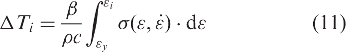

Stress relaxation (strain rate = 0)

Stress-relaxation tests

Relaxation in a viscoelastic material can be described by two parameters: characteristic relaxation time and equilibrium stress. A series of relaxation tests as a function of strain rates and temperatures were conducted to determine these parameters. Specimens were monotonically loaded at different strain rates (0.001, 0.01, and 0.1/s), and the displacement was held constant for 10 min at different strain levels (13, 18, and 31%). When a viscoelastic material is loaded at a certain strain rate, the resulting stress is always higher than the equilibrium stress. If the strain is kept constant, the material will relax, and the stress will decrease and approach the equilibrium stress asymptotically over time.

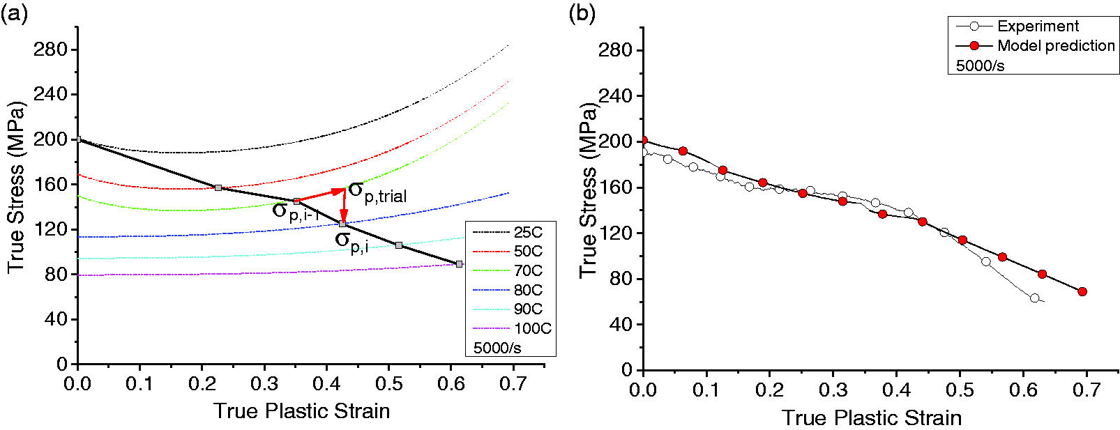
Figure 8(a) shows the stress–strain response for stress-relaxation tests conducted at 90 ℃ at different strain rates. When the strain is held constant, stress relaxes to the same equilibrium stress regardless of the applied strain rate. While reloading at a constant strain rate, the stress increases at a slope of the initial elastic modulus (at the chosen strain rate) until it reaches a maximum point, which appears exactly like the initial yield point. The material then softens and finally merges with the original stress–strain curve which was monotonically loaded without any interruption.

Figure 8.

(a) Under different strain rates, stress-relaxation tests are carried out at different strain levels (dotted lines). Stress–strain response at 90 ℃ under monotonic loading (0.001/s strain rate) is shown for comparison and (b) stress time plot shows strain rate-dependent relaxation.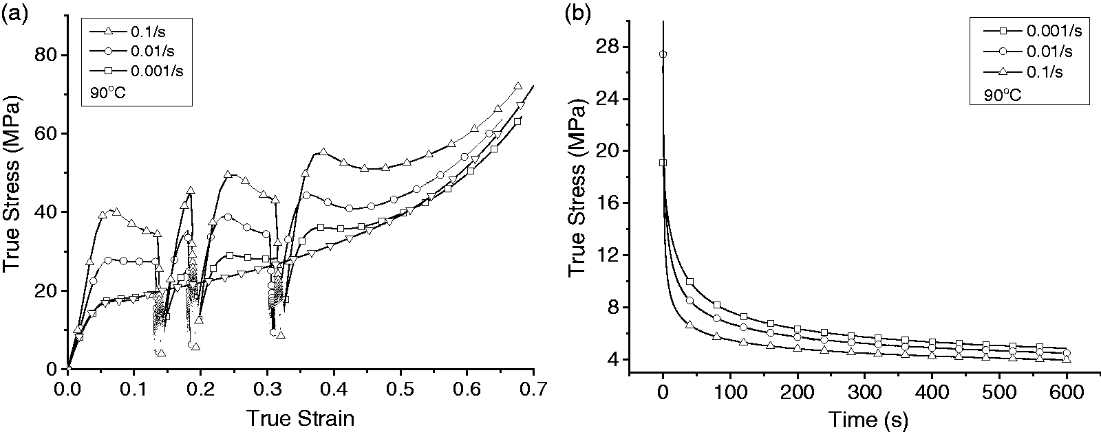

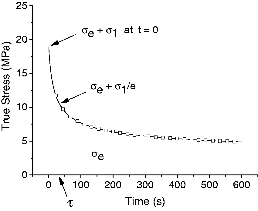
Figure 8(b) shows the relaxation curves for the same tests at 13% strain level. Characteristic relaxation time was determined by fitting the relaxation curves to an analytical solution (equation (13)) of a standard spring and dashpot solid model (Figure 9).

σ (\overset{\cdot}{ɛ}, T, t) = σ_{e} (T) + σ_{1} exp (- \frac{t}{τ (\overset{\cdot}{ɛ})})

(13)

where

σ_{e}

is the equilibrium stress and τ is the characteristic relaxation time. Relaxation time was found to be dependent only on the applied strain rate, which decreased with increasing strain rate. Equation for the strain rate-dependent relaxation time and the corresponding fitting parameters are presented in equation (14) and Table 6, respectively.

Figure 9.

Characteristic relaxation times are calculated based on analytical solution of a standard solid model.

Table 6.

Curve-fitting parameters for stress equilibrium path.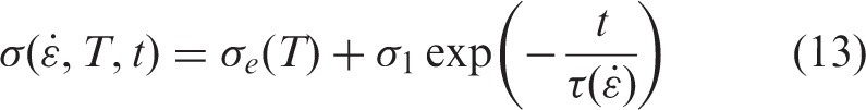

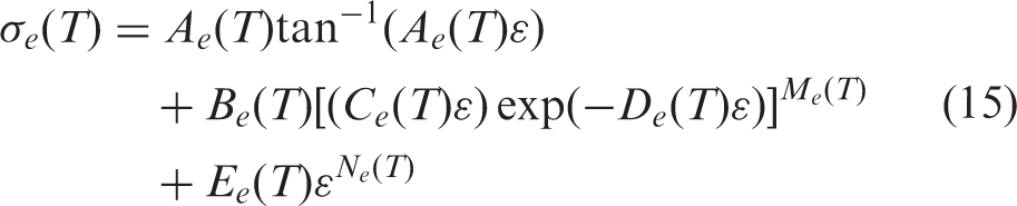
$a_{e}$	−0.418	$b_{e}$	0.695
	Test temperature (℃)
	25 ℃	50 ℃	70 ℃	80 ℃	90 ℃	100 ℃	110–150 ℃
$A_{e}$	30	21.3	14.41	10.34	7.49	4.02	3.63
$B_{e}$	49.78	36.22	34.9	11.17	2.00 × 10¹⁴	−1.37 × 10¹⁴	−1.29 × 10¹⁵
$C_{e}$	54.1	54.96	53.8	44.62	7.28 × 10¹⁶	2.7 × 10¹⁵	4.00 × 10¹⁶
$D_{e}$	22.64	21.95	26.45	18.96	4.77 × 10¹⁸	5.23 × 10¹⁶	4.59 × 10¹⁷
$E_{e}$	1.246	1.25	1.32	1.65	1.05 × 10²⁵	6.15 × 10²¹	4.55 × 10²¹
$M_{e}$	183.6	145.92	144.3	120.08	47.33	43.53	36.4
$N_{e}$	3.4	3.4	3.7	3.64	3.29	3.51	3.58

Stress equilibrium path was also determined at different temperatures (25–90 ℃) through a series of stress relaxation at several strain levels. Force–displacement response to obtain stress equilibrium paths at 50 ℃ is presented in Figure 10. The resulting equilibrium stress–strain response was fitted with an appropriate equation (equation (15)), and the corresponding fitting parameters are presented in Table 6.

Figure 10.

Raw load–displacement response from a series of stress relaxation tests was carried out to determine the stress equilibrium path. Dotted line shows the curve fitted to the equilibrium path.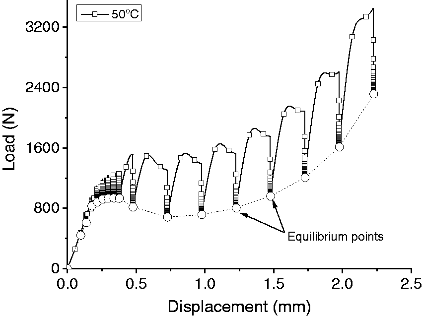

Modeling stress relaxation

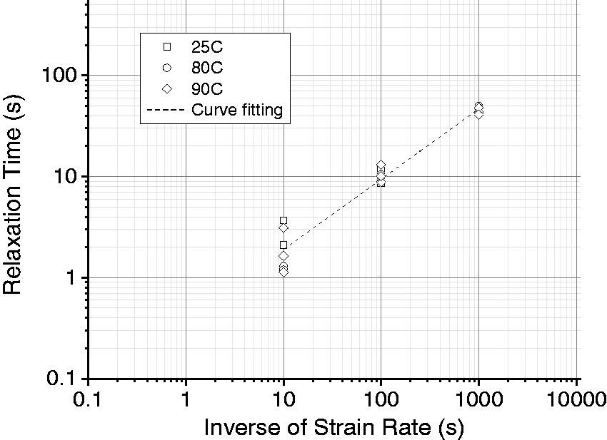
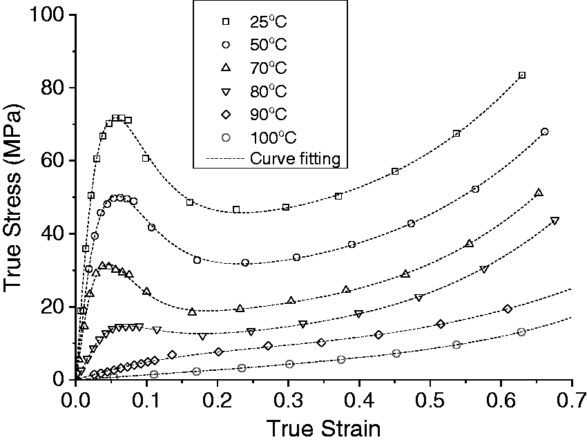
Experimental results showed that the characteristic relaxation time for epoxy resin DER 353 is significantly affected by the applied strain rate. The material relaxed quickly (reduced relaxation time) with the increase in applied strain rate. When plotted on a log–log scale, relaxation time and inverse of strain rate have a linear relation (Figure 11), which can be used to estimate the relaxation time for higher strain rates (equation (14)). The stress equilibrium paths (Figure 12), which depend on the temperature and strain level to which the material was deformed, was described using equation (15). The parameters used to fit the relaxation and stress equilibrium curves are presented in Table 6.

τ (\overset{\cdot}{ɛ}) = 10^{a_{e} + b_{e} log (\frac{1}{\overset{\cdot}{ɛ}})}

(14)

\begin{matrix} σ_{e} (T) = A_{e} (T) tan - 1 (A_{e} (T) ɛ) \\ + B_{e} (T) [(C_{e} (T) ɛ) exp (- D_{e} (T) ɛ)] M_{e} (T) \\ + E_{e} (T) ɛ^{N_{e} (T)} \end{matrix}

(15)

Figure 11.

Relaxation time shows linear relation with inverse of strain rate on a log–log plot.

Figure 12.

Curve-fitting stress equilibrium path at different temperatures (hollow dots represent experimental data points).

Unloading (strain rate < 0), reloading, and change in strain rate

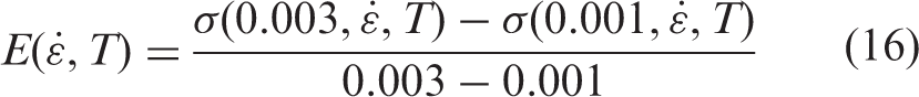
Unloading occurs at a slope comparable to the initial elastic modulus. Consequently, unloading after the material has yielded results in plastic deformation. An example of this can be seen in the unloading portion of the high rate stress–strain response (Figure 3(b)). In the model, when the strain rate becomes negative, the slope of the curve is calculated for the unloading strain rate at the given temperature using equation (16).

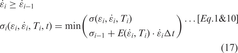
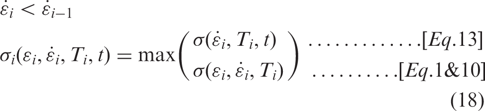
Similarly, when reloading or while increasing the strain rate abruptly during loading from any given strain level, the stress does not jump instantly to a lower value corresponding to the lower strain rate as would be predicted by standard models such as Johnson–Cook model. Instead, the stress follows the path of the slope of the elastic modulus (equation (16)) until the curve intersects the stress–strain path for the material which is loaded monotonically. The logic presented in equation (17) is used for such loading conditions. If the strain rate is decreased compared to the previous time step, the material relaxes (first term in equation (18)) until the stress values decreases to the ones corresponding to the lower strain rate, after which it follows the path for the new strain rate

\begin{matrix} E (\overset{\cdot}{ɛ}, T) = \frac{σ (0.003, \overset{\cdot}{ɛ}, T) - σ (0.001, \overset{\cdot}{ɛ}, T)}{0.003 - 0.001} \end{matrix}

(16)

\begin{matrix} {\overset{\cdot}{ɛ}}_{i} \geq {\overset{\cdot}{ɛ}}_{i - 1} \\ σ_{i} (ɛ_{i}, {\overset{\cdot}{ɛ}}_{i}, T_{i}, t) = min (\begin{matrix} σ (ɛ_{i}, {\overset{\cdot}{ɛ}}_{i}, T_{i}) \\ σ_{i - 1} + E ({\overset{\cdot}{ɛ}}_{i}, T_{i}) \cdot {\overset{\cdot}{ɛ}}_{i} Δ t \end{matrix}) \begin{matrix} \dots [Eq . 1 & 10] \end{matrix} \end{matrix}

(17)

\begin{matrix} {\overset{\cdot}{ɛ}}_{i} < {\overset{\cdot}{ɛ}}_{i - 1} \\ σ_{i} (ɛ_{i}, {\overset{\cdot}{ɛ}}_{i}, T_{i}, t) = max (\begin{matrix} σ ({\overset{\cdot}{ɛ}}_{i}, T_{i}, t) \\ σ (ɛ_{i}, {\overset{\cdot}{ɛ}}_{i}, T_{i}) \end{matrix}) \begin{matrix} \dots \dots \dots \dots . [Eq . 13] \\ \dots \dots \dots . [Eq . 1 & 10] \end{matrix} \end{matrix}

(18)

Model predictions

Model predictions for different loading cases are presented in this section. Figure 13 shows the temperature-dependent stress–strain prediction for monotonic loading at a strain rate of 0.001/s. The initial non-linear stress–strain response up to yield resulting from temperature-dependent viscoelastic behavior is accurately predicted by the spring and dashpot models. Prediction of temperature and strain rate-dependent yield stress using Ree–Eyring equation is critical here as it influences the post yield response and links the elastic and plastic behavior. Figure 6(b) shows good agreement in the prediction of yield stresses, and Figure 13 shows that these yield stresses can be used for the construction of smooth stress–strain curves linking elastic and plastic region. Post yield softening is present up to 70 ℃, which is followed by strain hardening. Appropriate equations are employed to ensure that the post yield softening begins to vanish at higher temperatures, and linear interpolations are used, so that the curves do not intersect with each other for different temperatures.

Figure 13.

Model prediction for stress–strain response at different temperatures under quasi-static (0.001/s) loading rate.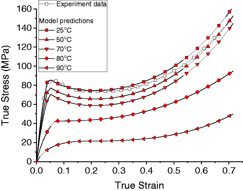

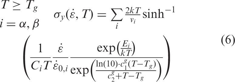
For temperatures above the T_g range (i.e. above 100 ℃), the yield stress becomes zero when subjected to a strain rate of 0.001/s (Figure 4). However, as the strain rate is increased, the epoxy resin starts to exhibit glassy behavior even above 100 ℃. Prediction of this behavior is presented in Figure 14, where the material exhibits a distinct yield stress at 100 ℃ under 0.1/s strain rate. Model prediction for the yield point at 0.1/s strain rate is slightly higher because the overall yield stress predicted by Ree–Eyring model is higher for this temperature (Figure 6(a)). This could be because only the initial value of the T_g range was used in determining the model parameters. It should be noted that the T_g range (including the initiation point) is also dependent on the strain rate, which was not accounted for in this study. For more accurate model predictions, the Ree–Eyring model with WLF equation (equation (6)) would need to be modified to account for strain rate-dependent T_g.

Figure 14.

Independent correlation between experimental results (hollow dots) and model predictions (solid red dots) for stress–strain response at 100 ℃ under 0.001 and 0.1/s strain rate.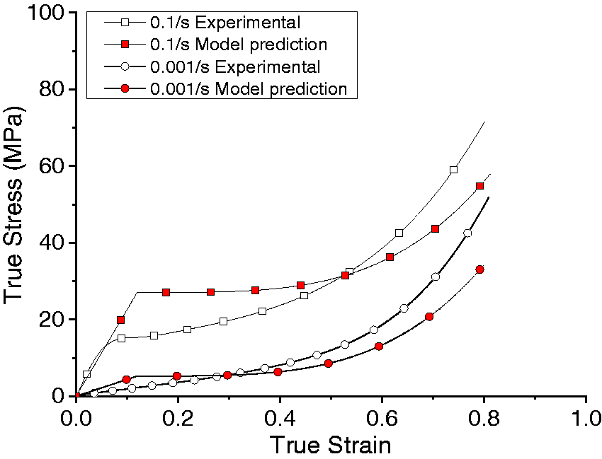

Comparison between model prediction and experimental results for temperature 110 and 120 ℃ under a strain rate of 0.001/s is shown in Figure 15. As evidenced from the experiments,³⁹ the same curve will be used for temperatures up to 150 ℃ at 0.001/s strain rate. For higher strain rates, the curves are shifted vertically depending on the yield stress predicted by Ree–Eyring equation for the given temperature and strain rate.

Figure 15.

Independent correlation between experimental result (hollow dots) and model prediction (solid red dots) for stress–strain response under a strain rate of 0.001/s at (a) 110 and (b) 120 ℃.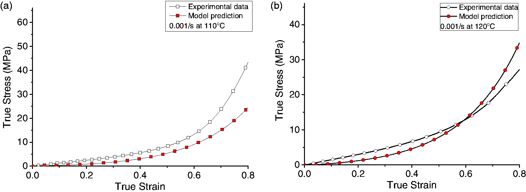

Model prediction for strain rates 0.00–0.1/s at 25 ℃ is shown in Figure 16. The overall trend of the post yield response—softening, plastic flow, and hardening—is the same for all strain rates. For higher strain rates $(\overset{\cdot}{ɛ} > 1000 / s)$ , strain hardening is completely absent due to thermal softening caused by adiabatic heating during loading. Softening becomes more dramatic when the material approaches the glass transition temperature $(T_{g})$ , and this point occurs progressively at smaller strain level as the strain rate is increased (Figure 16). Comparison between model prediction and experimental results conducted independently shows an excellent agreement at the strain rate of 5000/s (Figure 7). Model prediction up to a strain rate of 10⁶/s is presented in Figure 16.

Figure 16.

Stress–strain prediction at strain rates (a) 0.001–0.1/s and (b) 10³–10⁶/s shows thermal softening, which becomes more prominent and starts to occur at lower strain levels with increasing strain rate.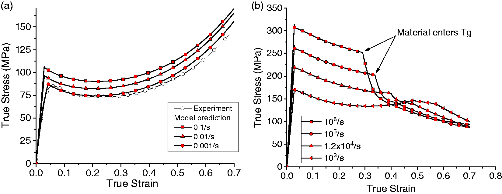

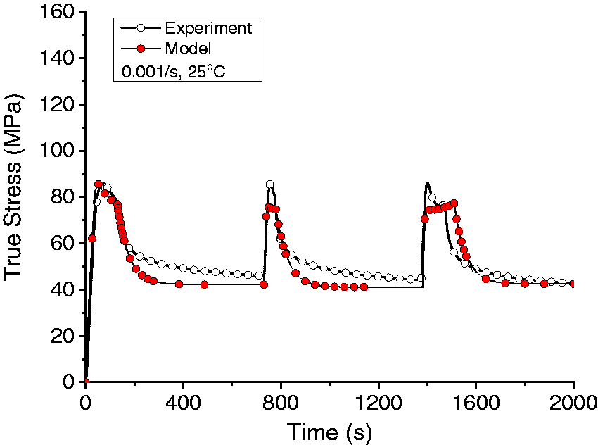
Strain–time input profile for stress-relaxation test at 25 ℃ is shown in Figure 17(a). Applied strain rate is 0.01/s, which is interrupted at different strain levels (0.13, 0.18, and 0.31) with zero strain rate. Model prediction shows stress relaxation approaching equilibrium stress when the displacement is held constant. While reloading, the stress increases at a slope, E, corresponding to the applied strain rate until the curve intersects with the path which would have occurred, had the material been loaded monotonically without interruption. The same rule applies during strain rate jumps. This phenomenon is confirmed by the experimental results where the material is reloaded after stress relaxation (Figure 17(b)). Prediction of stress–time plot for stress-relaxation tests at 0.001/s shows decay of stress to the equilibrium point (Figure 18). The model underestimates the peaks because during the experiment, when reloading occurs, the material is elastically loaded and yields, which is again followed by post yield softening. Since this behavior was not captured in the model, the peaks are underestimated after reloading. The discrepancy in relaxation part of the curve in Figure 18 can be attributed to the use of one relaxation time for all temperatures employed for the given strain rate as shown by curve fitting in Figure 11.

Figure 17.

(a) Input strain–time profile for stress-relaxation tests at strain rate of 0.01/s and (b) model prediction with relaxation at 13, 18, and 31% strain level.

Figure 18.

Model output shows good correlation with stress-relaxation experiment for stress time curve.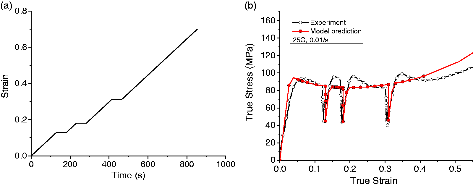

A case study for variable strain rate with a sudden jump in strain rate at elastic and plastic region during monotonic loading is presented in Figure 19 (analogous to a fiber break discussed in the “Introduction” section). The strain rate is increased from 0.001 to 1/s at different strain levels. The response of our model is compared to Johnson Cook in Figure 19(b). Immediately, following the change in strain rate, current model prediction shows the stress increasing at a slope, E corresponding to the new strain rate until it crosses path with the monotonically loaded curve as explained earlier. In contrast, Johnson Cook model prediction shows sudden increment in stress value instead of increasing at the slope of the modulus.

Figure 19.

(a) Input strain time profile for strain rate jump tests. Strain rate is suddenly increasing from 0.001 to 0.1/s and (b) model prediction for strain rate jump tests.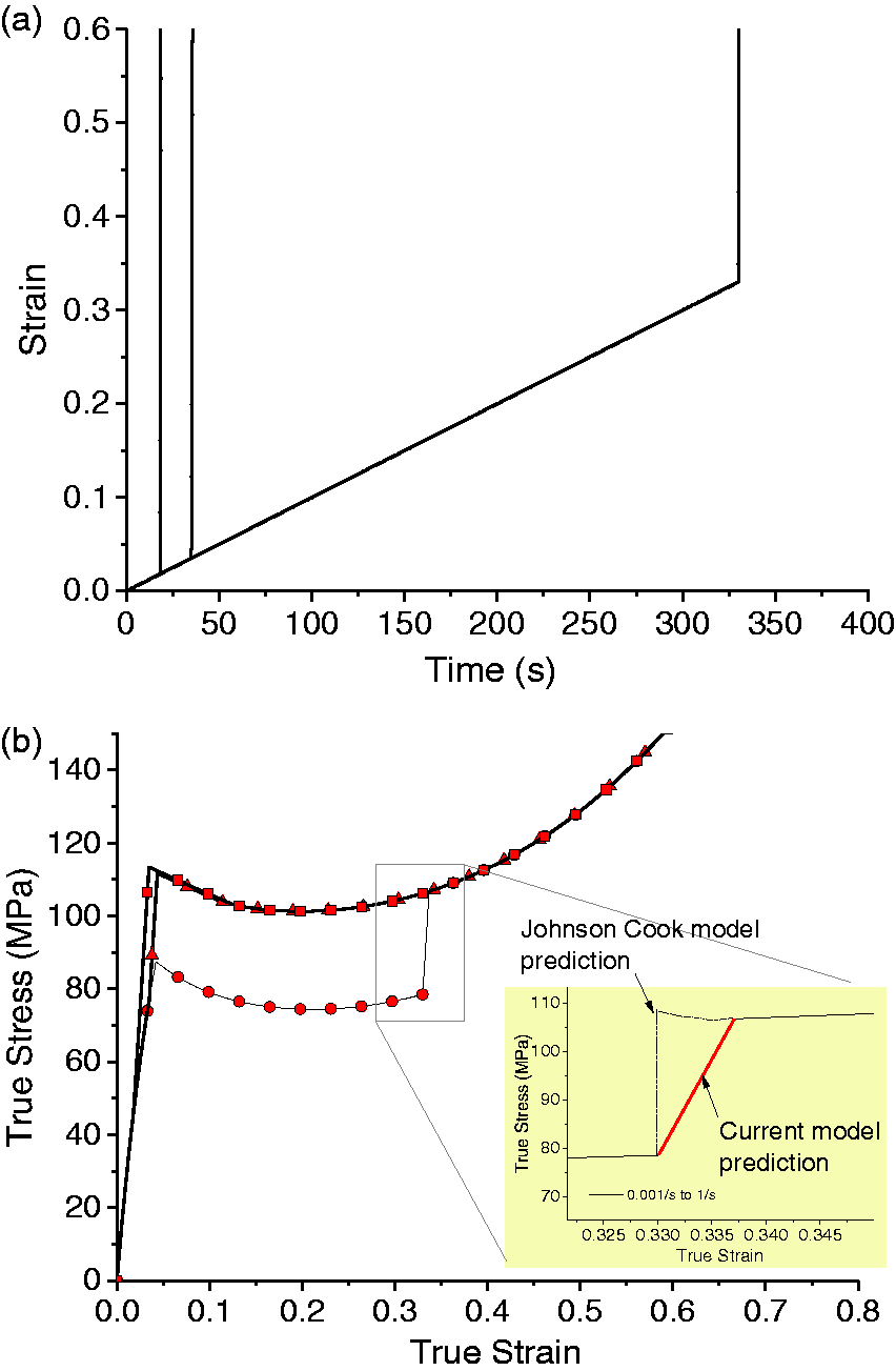

Similarly, a case for sudden reduction in strain rate from 0.01 to 0.001/s is shown in Figure 20. Red curve shows stress–time path when stress relaxation occurs. When the strain rate is suddenly decreased, the stress–time response decays and follows the stress-relaxation curve until the stress intersects the value corresponding to the lower (0.001/s) strain rate. After this point, the model predicts stress values for monotonically loaded curve at the lower strain rate. Comparison with Johnson Cook model shows stress prediction decreasing instantaneously to the lower strain rate value since Johnson Cook model does not account for stress relaxation. The importance of these differences will likely depend on the problem being solved and is a focus of our future studies.

Figure 20.

Comparison in stress–time prediction for Johnson Cook model and current model when changing the strain rate suddenly from 0.01 to 0.001/s.

Finally, model prediction for load–unload case at 0.001/s strain rate is presented in Figure 21. When unloading occurs, the stress values decrease at a slope, E, regardless of whether the material is in elastic or plastic region.

Figure 21.

(a) Input strain–time profile for load–unload tests and (b) model prediction for load–unload tests at elastic and plastic region.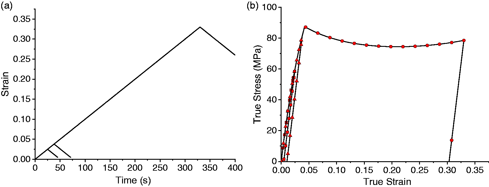

Conclusions

Time and temperature-dependent model to predict uniaxial compressive behavior of an epoxy resin was developed using an incremental approach. Stress–strain response under monotonic loading is decomposed into elastic and plastic region. Strain rate and temperature-dependent yield stress, which is predicted using Ree–Eyring equation, links the two regimes to construct a contiguous stress–strain curve. The initial stress–strain response and the plastic response are modeled using empirical as well as physically based spring and dashpot models. To determine the model parameters, temperature–dependent properties of DER 353 were characterized in uniaxial compression mode under various strain rates. A series of stress-relaxation tests were also carried out for the determination of characteristic relaxation time and equilibrium stress state. The model is able to predict stress–strain response for monotonic and varying strain rates in loading and unloading scenario. Thermal softening in the stress–strain curve at large strains, which is inevitable at higher strain rates, is also predicted by estimating the rise in temperature of the material during each increment in loading. Moreover, the model can also predict relaxation in stress values when the strain rate drops to zero after the material has been loaded to a certain strain level. Model prediction for different loading scenarios show an excellent correlation when compared to the experimental results.

Footnotes

Acknowledgements

The research was sponsored by the Army Research Laboratory and was accomplished under Cooperative Agreement Number W911NF-12-2-0022. The views and conclusions contained in this document are those of the authors and should not be interpreted as representing the official policies, either expressed or implied, of the Army Research Laboratory or the U.S. Government. The U.S. Government is authorized to reproduce and distribute reprints for Government purposes notwithstanding any copyright notation herein.

Declaration of Conflicting Interests

The author(s) declared no potential conflicts of interest with respect to the research, authorship, and/or publication of this article.

Funding

The author(s) received no financial support for the research, authorship, and/or publication of this article.

References

Biron

. Thermosets and composites: material selection, applications, manufacturing and cost analysis, Amsterdam, Netherlands: Elsevier, 2013.

Gupta

Drzal

Lee

CY-C

, et al. The temperature dependence of some mechanical properties of a cured epoxy resin system. Polym Eng Sci 1985; 25: 812–823.

Panda

. Epoxy resins technology handbook (manufacturing process, synthesis, epoxy resin adhesives and epoxy coatings), Delhi: Asia Pacific Business Press, 2016.

Zaera R. Ballistic impacts on polymer matrix composites, composite armor, personal armor. In: Impact engineering of composite structures. Vienna: Springer, 2011, pp.305–403.

Liu

Zheng

. Recent developments on damage modeling and finite element analysis for composite laminates: a review. Mater Des 2010; 31: 3825–3834.

Karger-kocsis

Mahmood

Pegoretti

. Recent advances in fiber/matrix interphase engineering for polymer composites. Prog Mater Sci 2015; 73: 1–43.

Pimenta S. Fibre failure modelling. In: Camanho PP and Hallett SR (eds) Numerical modelling of failure in advanced composite materials. Cambridge, UK: Woodhead Publishing, 2015, pp.193–224.

Mishnaevsky

Brøndsted

. Micromechanisms of damage in unidirectional fiber reinforced composites: 3D computational analysis. Compos Sci Technol 2009; 69: 1036–1044.

Swolfs

Verpoest

Gorbatikh

. A review of input data and modelling assumptions in longitudinal strength models for unidirectional fibre-reinforced composites. Compos Struct 2016; 150: 153–172.

10.

Ganesh

Sockalingam

(Gama) Haque

, et al. Dynamic effects of single fiber break in unidirectional glass fiber-reinforced composites. J Compos Mater. 2017; 51(9): 1307–1320.

11.

Swolfs

Gorbatikh

Verpoest

. Fibre hybridisation in polymer composites: a review. Compos Part A Appl Sci Manuf 2014; 67: 181–200.

12.

Sockalingam

Dey

Gillespie

, et al. Finite element analysis of the microdroplet test method using cohesive zone model of the fiber/matrix interface. Compos Part A Appl Sci Manuf 2014; 56: 239–247.

13.

Tamrakar S, Sockalingam S, Haque BZ, et al. High strain rate fiber matrix interface characterization - Experimental testing and finite element analysis. In: SAMPE, Seattle, 2–5 June 2014.

14.

Tamrakar

Haque

Gillespie

. High rate test method for fiber-matrix interface characterization. Polym Test 2016; 52: 174–183.

15.

Tamrakar

Thostenson

, et al. Tailoring interfacial properties by controlling carbon nanotube coating thickness on glass fibers using electrophoretic deposition. ACS Appl Mater Interf 2016; 8: 1501–1510.

16.

Mahieux

Reifsnider

. Property modeling across transition temperatures in polymers: A robust stiffness-temperature model. Polymer (Guildf) 2001; 42: 3281–3291.

17.

Richeton

Schlatter

Vecchio

, et al. A unified model for stiffness modulus of amorphous polymers across transition temperatures and strain rates. Polymer (Guildf) 2005; 46: 8194–8201.

18.

Lubarda

Benson

Meyers

. Strain-rate effects in rheological models of inelastic response. Int J Plast 2003; 19: 1097–1118.

19.

Plaseied

Fatemi

. Deformation response and constitutive modeling of vinyl ester polymer including strain rate and temperature effects. J Mater Sci 2008; 43: 1191–1199.

20.

Yao

Han

, et al. A visco-elastoplastic constitutive model for large deformation response of polycarbonate over a wide range of strain rates and temperatures. Polymer (UK) 2014; 55: 6577–6593.

21.

Bauwens-Crowet

Bauwens

Homès

. The temperature dependence of yield of polycarbonate in uniaxial compression and tensile tests. J Mater Sci 1972; 7: 176–183.

22.

Roetling

. Yield stress behaviour of poly(ethyl methacrylate) in the glass transition region. Polymer (Guildf) 1965; 6: 615–619.

23.

Haward R. The physics of glassy polymers, https://books.google.com/books?hl=en&lr=&id=lOvqCAAAQBAJ&oi=fnd&pg=PR10&dq=physics+of+glassy+polymers&ots=qzVWwOneeT&sig=b8k0KLfU3Hh3vDaYh2bx-oQ56NM (2012, accessed 4 May 2017).

24.

Gómez-del Río

Rodríguez

. Compression yielding of epoxy: strain rate and temperature effect. Mater Des 2012; 35: 369–373.

25.

Haward RN. The physics of glassy polymers. Berlin, Germany: Springer Science & Business Media, 2012.

26.

Roetling

. Yield stress behaviour of polymethylmethacrylate. Polymer (Guildf) 1965; 6: 311–317.

27.

Mulliken

Boyce

. Mechanics of the rate-dependent elastic-plastic deformation of glassy polymers from low to high strain rates. Int J Solids Struct 2006; 43: 1331–1356.

28.

Richeton

Ahzi

Daridon

, et al. A formulation of the cooperative model for the yield stress of amorphous polymers for a wide range of strain rates and temperatures. Polymer (Guildf) 2005; 46: 6035–6043.

29.

Nemes

Spéciel

. Use of a rate-dependent continuum damage model to describe strain-softening in laminated composites. Comput Struct 1996; 58: 1083–1092.

30.

Frantziskonis

Desai

. Constitutive model with strain softening. Math Comput Model 1987; 23: 733–750.

31.

Van Breemen

LCA

Engels

TAP

Klompen

ETJ

, et al. Rate- and temperature-dependent strain softening in solid polymers. J Polym Sci Part B: Polym Phys 2012; 50: 1757–1771.

32.

Van Melick

HGH

Govaert

Meijer

HEH

. On the origin of strain hardening in glassy polymers. Polymer (Guildf) 2003; 44: 2493–2502.

33.

Govaert

Engels

TAP

Wendlandt

, et al. Does the strain hardening modulus of glassy polymers scale with the flow stress?. J Polym Sci Part B: Polym Phys 2008; 46: 2475–2481.

34.

Hoy

Robbins

. strain hardening of polymer glasses: effect of entanglement density, temperature, and rate. J Polym Sci Part B Polym Phys 2006; 44: 3487–3500.

35.

Hoy

Robbins

. Strain hardening in polymer glasses: limitations of network models. Phys Rev Lett 2007; 99: 1–4.

36.

Arruda

Boyce

Jayachandran

. Effects of strain rate, temperature and thermomechanical coupling on the finite strain deformation of glassy polymers. Mech Mater 1995; 19: 193–212.

37.

Pan

Sun

Shim

VPW

, et al. Transient heat generation and thermo-mechanical response of epoxy resin under adiabatic impact compressions. Int J Heat Mass Transf 2016; 95: 874–889.

38.

Bergstrom

. Constitutive modeling of the large strain time-dependent behavior of elastomers. J Mech Phys Solids 1998; 46: 931–954.

39.

Tamrakar

Ganesh

Sockalingam

, et al. Experimental investigation of strain rate and temperature dependent response of an epoxy resin undergoing large deformation. J Dyn Behav Mater 2018; 4: 114–128.

40.

Jang

Sharifi

Palmese

, et al. Crosslink network rearrangement via reactive encapsulation of solvent in epoxy curing: a combined molecular simulation and experimental study. Polymer (UK) 2014; 55: 3859–3868.

41.

Tamrakar S. Characterization of S-glass epoxy composite interface under various rates of loading. PhD Dissertation. University of Delaware, DA, USA, 2018.