
Abstract
Theoretical details of two failure criteria implemented in an orthotropic plasticity model are presented. Improvements to the well-known Puck Failure criterion and a recently developed Generalized Tabulated Failure criterion are used to illustrate how to link a failure sub-model to existing deformation and damage sub-models in the context of explicit finite element analysis. These models are implemented in LS-DYNA, a commercial transient dynamic finite element code. Two validation tests are used to evaluate the failure sub-model implementation and improvements - a stacked-ply test carried out at room temperature under quasi-static tensile and compressive loadings, and a high-speed, projectile impact test where there is significant damage and material failure of the impacted panel. Results indicate that developed procedures and improvements provide the analyst with a reasonable and systematic approach to building predictive impact simulation models.
Introduction
Amongst several key topics in building an end-to-end predictive modeling framework for composites, three focus areas are: predictions of elastic and plastic deformation, damage initiation and progression, and the failure of structural systems subjected to quasi-static and impact loads. In addition to the complexity of accurately simulating the deformation and damage response of composites, accurately predicting composite failure, particularly in the context of a structural analysis, is a huge challenge. For example, composites fail in compression in a variety of ways – fiber crushing, splitting, elastic microbuckling, matrix failure and plastic microbuckling, buckle delamination, shear-band formation, etc. There are other modes of failure involving fracture of the material that is brought about by fiber breakage, fiber micro-buckling, fiber pullout, matrix cracking, delamination, debonding, or any combination of these mechanisms. In fact, after three Worldwide Failure Exercises that started in the early 1990s, the consensus is that there exist several damage and failure theories none of whom are capable of “…predicting all the strength and deformation of the lamina and laminates within 10% of the measured data”. 1
The architecture of even the simplest composite leads to a complex state of stress in structural systems. While unidirectionally loaded test specimens yield important stress-strain data in the Principal Material Directions (PMDs), the damage and failure states obtained from the test results are for the most part, for simple states of stress. The interaction between different states of stress are captured by higher level theories, such as Tsai-Wu, for predicting when the material would yield and how the yield surface would evolve. 2 However, the damage and failure theories lack the resolution to accurately predict damage and especially failure, at the continuum scale where the composite architectural details are missing. While there is widespread consensus that these architectural details need to be a part of the structural analysis process, there is no consensus as to how to define them and then how to use them at the appropriate scale primarily because of the enormous computational expense in carrying out multi-scale and multi-level finite element (FE) computations.
An orthotropic elasto-plastic damage material model suitable for impact analysis of composite materials has been developed through a joint research project funded by the Federal Aviation Administration and the National Aeronautics and Space Administration.3–6 The material model is implemented into LS-DYNA 7 as MAT_ COMPOSITE_TABULATED_PLASTICITY_ DAMAGE, also known as MAT_213. MAT_213 is a constitutive model with a modular architecture comprised of three sub-models - deformation, damage and failure. The deformation sub-model predicts the linear and the non-linear response of a composite and is driven by a set of tabulated stress-strain data set. The damage sub-model predicts the reduction in the stiffness of the material. The failure sub-model predicts when there is no more load carrying capacity in the FE, carries out the computations for a gradual decrease in the stiffness of the element, and tags the element for erosion from the FE model.
In an earlier work, 3 the well-known Puck Failure Criterion (PFC) was discussed, verified and validated. PFC was implemented as a part of the failure sub-model in MAT_213. While obtaining all the required material parameters proved to be difficult, the results from the validation exercises were encouraging. Some numerical calibration was necessary to obtain realistic results. In this paper, some of the shortcomings of PFC are discussed and modifications to the theory and implementation are introduced especially with respect to post-peak/post-failure simulation so that a stable post-peak behavior can be achieved. In addition, a (new) second failure model, the Generalized Tabulated Failure Criterion (GTFC) 8 as implemented in MAT_213, is discussed. This model is built with user input that define the two modes of failure – in-plane and out-of-plane modes. In the context of this paper, the term failure onset implies the instant at which there is no further increase in the load carrying capacity exhibited by the finite element, and the term erosion refers to the deletion of the finite element from further model calculations. The first part of the paper discusses the relevant parts of the deformation and damage sub-models. It is shown that the damage sub-model can be used not only for handling pre-peak damage state, but also can be used to affect post-peak behavior. The second part of the paper shows the improvements made to both PFC and GTFC. The discussions center around the required input, onset of failure detection, and post-peak behavior including (finite) element erosion. Numerical examples form the next section of the paper. A quasi-static stacked ply test and a high-velocity impact test of a flat panel are used as validation tests for the developed and improved constitutive models. The paper concludes with discussions on how some of the modeling challenges were overcome and what can be done to further improve these models.
Deformation and damage Sub-Models
A minimum of twelve stress-strain input curves are required to drive the deformation sub-model. The stress-strain input curves include (a) tension and compression curves in the 1, 2 and 3 PMDs, (b) shear curves in the 1–2, 2–3 and 1–3 Principal Material Planes, and (c) three 45° off-axis tension/compression curves in the Principal Material Planes. When available, additional stress-strain curves at different strain-rate and temperature combinations can also be specified. A general three-dimensional stiffness matrix is used where the components are obtained from the user input stress-strain curves for the current strain-rate and temperature in the finite element.4–6,9 The onset of plasticity is predicted using a yield function which is a modified form of the Tsai-Wu failure criterion. The yield function coefficients are computed based on the current flow stress. The direction of the plastic flow is dictated by a quadratic plastic potential function.
The damage sub-model predicts the reduction in the stiffness of the material assuming strain equivalence between the true and the effective stress spaces.10,11 The true stress space corresponds to the damaged state whereas the effective space corresponds to the undamaged state. Strain equivalence assumption allows the damage sub-model to predict the reduction in the stiffness without affecting the deformation sub-model. The true stress
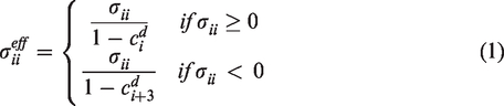
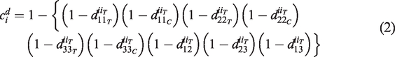
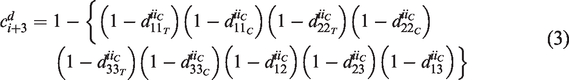
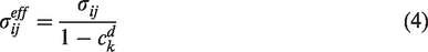

The plasticity algorithm works in the effective stress-space in order to uncouple the deformation and the damage sub-models. 11 Therefore, all the stress-strain input curves which are in the true stress space are converted into the effective stress space using only the associated uncoupled damage parameters. The plastic multiplier is computed during the plasticity algorithm after which the stress is updated using a radial return scheme in the effective stress space. The effective stress tensor is ultimately converted back to the true stress space. This approach will be of importance when discussing the failure sub-models.
Failure modeling
In this section, two improved versions of failure theories are discussed - Puck Failure Criterion (PFC) and Generalized Tabulated Failure Criterion (GTFC). The reason for incorporating multiple failure theories in the same material model is that, as will be discussed later, each one of these criteria has its strengths and weaknesses. GTFC provides a relatively new concept for handling failure and is driven primarily by a user-defined failure envelope.
Puck failure criterion
Puck failure theory is a physically based failure model for unidirectional composites.12–14 It assumes that there is transverse isotropy in the material at the lamina level. The failure theory considers two modes of failure - Fiber Fracture (FF) and Inter Fiber Fracture (IFF). The implementation of PFC in MAT_213 has been discussed in an earlier publication. 3 The failure modes are used to predict the failure onset in the finite element. Furthermore, a stress degradation model (SDM) which gradually degrades the material behavior after failure onset, and ultimately predicts when element erosion needs to take place, is used. SDM helps avoid a sudden drop in the stress after failure onset thus providing not only numerical stability but also serves as a mesh regularization scheme.
The SDM discussed earlier
3
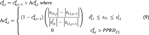
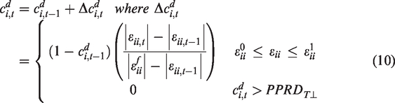
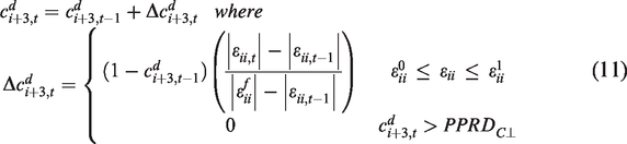
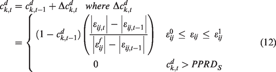
has been modified. In the previous implementation, at the element Gauss point under consideration, once failure onset is detected, the deformation and the damage calculations were skipped. The value of true stress corresponding to the failure onset was stored and was scaled down to compute the degraded stress. Sometimes this approach resulted in excessively elongated elements, smaller critical time step, and thereby longer simulation run time. In the improved implementation presented here, the computations related to deformation and damage are carried out even after failure onset. The effective stress is held constant, but the true stress is gradually reduced. This approach provides not only post-peak numerical stability but the ability to control the residual strength in the finite element. In the context of this paper, residual strength,
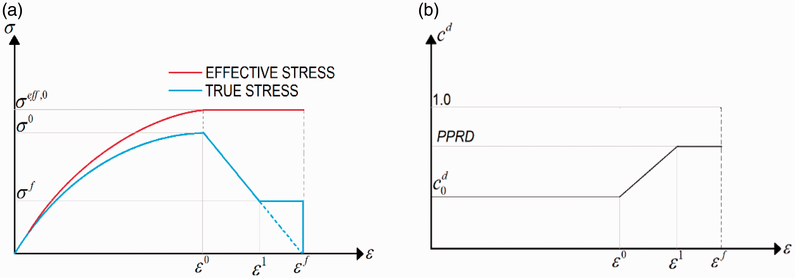
(a) Stress vs strain response using PFC (note
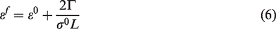
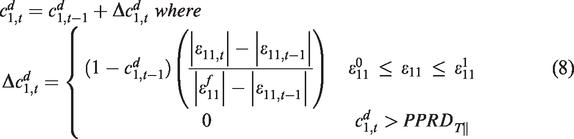
Equation (6) is based on the assumption that the area under the stress-strain curve between
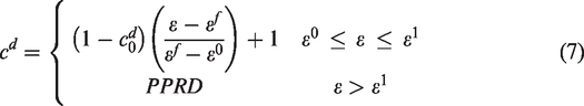
For
Twenty parameters are used in the PFC to detect failure onset, implement the SDM algorithm, and carry out element erosion. Most, not all, can be readily found from experiments. The tensile, compressive and shear strength parameters,
The algorithm used in PFC with the new SDM implementation is as follows.
If
For
If
For
When
(i) (ii)
where


When
(i)
(ii)
(iii)
Sometimes after an element is eroded, the neighboring elements undergoing the stress degradation process may experience sudden changes in the strain field due to stress redistribution. This process may lead to undesirable stress oscillations (stress reversals, tension to compression or vice versa) taking place in a very short duration of time. Criteria (ii) and (iii) in Step 2.2(b) erode the elements in which stress reversal with respect to the stress at the failure onset takes place. Since the PFC assumes transverse isotropy, care needs to be taken regarding which stress component (
Although Puck failure theory has been considered one of the better models in World-Wide Failure Exercise I (WWFE-I) and World-Wide Failure Exercise II (WWFE-II),20,21 there are limitations that should be noted. First, the theory is valid for transversely isotropic material at the lamina level. Second, the Master Fracture Body is not a closed envelope. 13 Third, the failure criteria are not functions of rate and temperature. This factor is important for unidirectional polymeric composites that exhibit rate and temperature sensitivities and form the impacted structural system.
Generalized tabulated failure criterion
A failure model where an arbitrarily shaped failure surface in the stress space can be used to predict the failure of a composite is highly desirable. One would expect the failure surface of a composite to be complex such that a mathematical expression cannot be defined and used as is done with traditional failure criteria.22,23 In the earlier version of GTFC, 8 the in-plane, the out-of-plane and the combined in-and-out-of-plane failure states were defined in terms of stresses. The current version of GTFC assumes that failure states are strain rather than stress-based so that post-peak behavior can be handled seamlessly. Failure surfaces need to be defined for each of these failure states in the equivalent failure strain and failure angle space. 24
Figure 2 shows the in-plane failure surface where

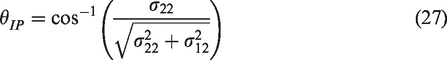
General form of in-plane failure surface.
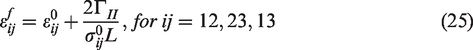
Note that the failure angle is expressed in terms of
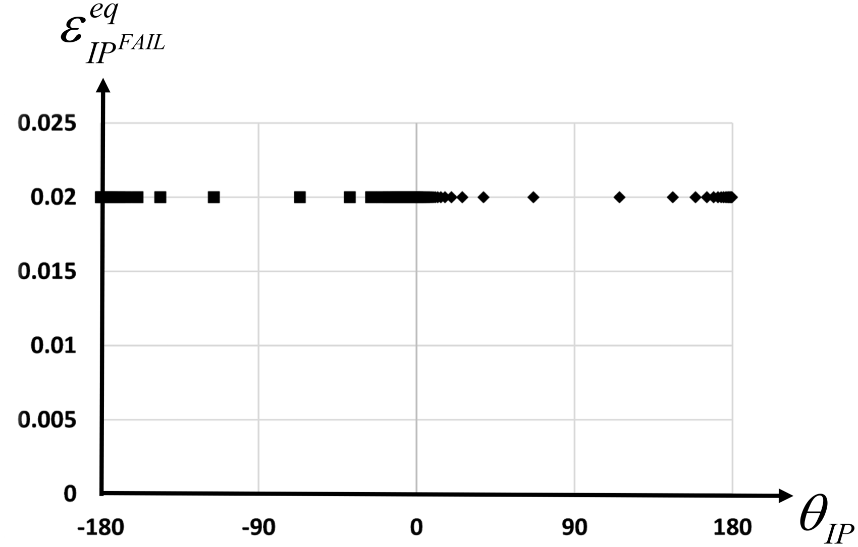
In-plane failure surface where failure angle is computed using
Let the in-plane failure state
An out-of-plane failure surface can be constructed similar to Figure 2 with the failure surface expressed in terms of

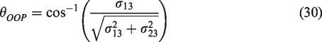
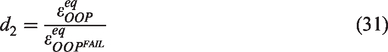
Similarly, the out-of-plane failure state
An element is eroded if
The algorithm used in GTFC is as follows.
Step 1: For a given time step, update the element Gauss point stress tensor using the deformation and the damage sub-models.
Step 2.1: Compute
Step 2.2: Compute
Step 3.1: Compute
Step 3.2: Compute
Step 4: Compute
Unlike PFC, GTFC does not require failure onset to be detected to compute the post-peak response. Each input stress-strain curve has a pre-peak and post-peak regime that are used to capture the peak stress via the deformation and damage sub-models, and handle the post-peak behavior via the damage sub-model similar to what is done with the stress degradation model in PFC. Figure 4(a) shows a typical stress-strain input curve for a given component. The portion of the stress data between
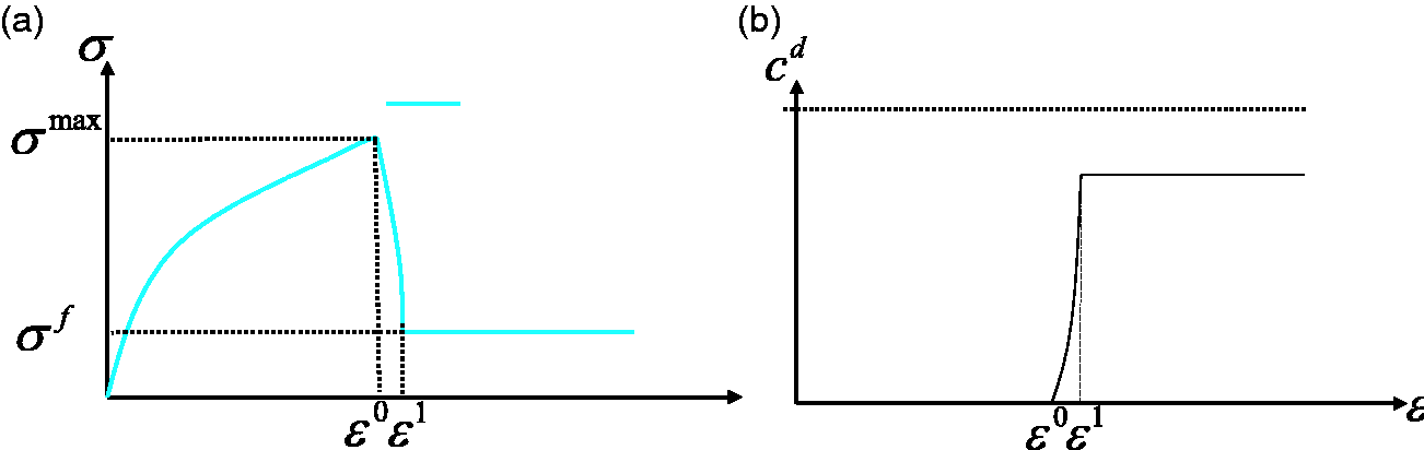
(a) Stress-strain input augmented with post-peak data (note
Like PFC, the current implementation of GTFC is not rate and temperature dependent. Obtaining experimentally a rich set of failure surface data is neither easy nor feasible with the current state-of-the-art. The combination of experimental testing along the principal material directions and virtual testing for combined states of stress appears to be a viable option. To alleviate this problem, in this paper, the in-plane and out-of-plane responses are computed separately and then combined via the interaction term,
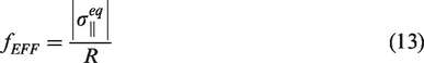
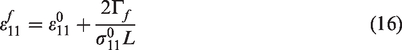
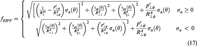
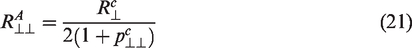
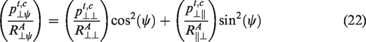
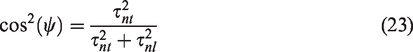
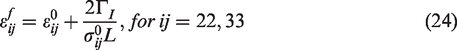
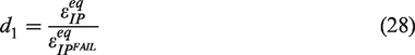
It should be noted that computation of the failure strain (strain at which element is eroded) is different for PFC and GTFC. In the case of the PFC, the failure strains are computed in the material model as soon as the element reaches the failure onset (Figure 1), and are computed separately for the FF mode (equation (16)) and the IFF mode (equations (24) and (25)). In the case of GTFC, the failure strains are specified as user input in the form of equivalent failure strains in the two modes: in-plane,
Numerical results
General Details: The verification and validation for both GTFC and PFC implementations were done using the T800/F3900 25 unidirectional composite. T800/F3900 is a carbon fiber composite with epoxy matrix and a fiber volume fraction of roughly 60%. Experiments show that the composite exhibits brittle failure with little or no post-peak strength.15,26 One-element verification tests are used to explain the implementation nuances of both failure criteria. Two validation tests are used to determine the efficiency and accuracy of the failure theories – a stacked-ply test carried out at Arizona State University (ASU) with loading in the quasi-static regime, and a high-velocity impact test carried out at National Aeronautics and Space Administration – Glenn Research Center (NASA-GRC). Three different mesh sizes have been used for the stacked-ply validation tests – coarse, medium, and fine with increasing mesh densities to study mesh dependencies and convergence properties. For the sake of brevity, details of the convergence analyses used in generating the optimal mesh (one that balances accuracy and computational cost) for the impact validation test are not presented here but can be found in Hoffarth et al. 9 In the impact validation tests, cohesive zone elements (CZE) have been used for modeling the delamination behavior and the details can be found in an earlier publication. 19
PFC Parameters: The same input parameters used in our previous research
3
are used here:
GTFC Parameters: For all the simulations using GTFC, it has been assumed that the compression residual strength parameters are equal to the respective peaks in the stress-strain input curves,
Numerical Calibration of Failure-related Parameters: As stated earlier, there are numerous failure-related parameters that can be altered to achieve better predictions. Amongst all failure-related parameters, the following parameters were used to improve the finite element predictions via a few trial-and-error runs: PFC:
Nomenclature: The following nomenclature is used in the numerical example graph legends: (a) MAT213-GTFC and MAT213-PFC imply that the simulation was run with GTFC and PFC, respectively, (b) the post-fixes -F, -M and -C imply that the simulation was run with fine, medium and coarse mesh model, respectively, (c) the post-fix -Modified Strength implies that one or more failure-related values have been calibrated, (d) Experiment implies experimental data from a single test replicate (e.g., impact test), (e) for all MAT213-PFC simulations, Model represents the processed data from the experimentally obtained stress-strain curves, 15 and (f) for all the MAT213-GTFC simulations, Model implies that calibrated post-peak stress-strain data is added to the experimentally obtained pre-peak data.
PFC single element verification test
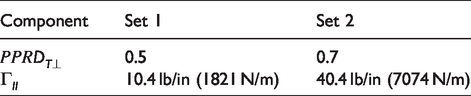
Background: One single-element example is discussed to illustrate the new SDM implementation. The example considered is 2-direction tension model. The test is executed with two different sets of input parameters that influence the post-peak behavior (Table 1).
Input parameters for verification.
Finite Element Modeling: The model involving the 8-noded hexahedral element is shown in Figure 5. The boundary conditions are applied in order to obtain a uniaxial state of stress in the 2-direction. The pin support represents restraints in all the three translational displacements. The crossed red color arrows represent a restraint in the translational displacement along the direction of the arrow. The black color arrows represent applied displacements.
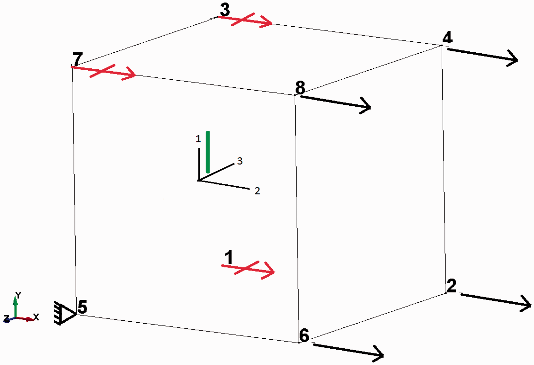
Schematic of 2-direction tension test model.
Results: The Model curve as well as the stress-strain response of the FE models are shown in Figure 6 where the effective damage parameter is shown using the secondary axis.
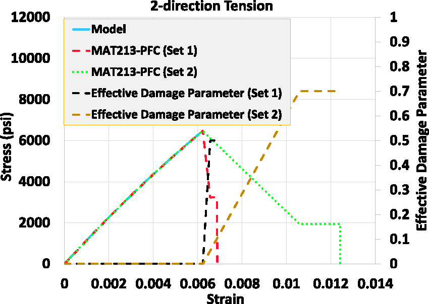
PFC input and results: 2-direction tension test stress and effective damage parameter versus strain response.
Discussions: The pre-peak stress-strain responses remain the same for Set 1 and Set 2. The difference is observed in the post-peak regime. The larger the value of
GTFC single element verification test
Background: This test is the same single element test used with the PFC, but now executed with GTFC.
Finite Element Modeling: As can be seen in Figure 7(a), there is an additional post-peak regime in the Model curve. As explained earlier, the stress-strain data in the pre-peak regime are obtained from experiments, whereas the stress-strain data in the post-peak regime are synthetic data that is used to control the post-peak stress degradation behavior. The figure also shows the effective damage parameter curve which increases from 0.0 to a value of 0.9 (see secondary axis), and the corresponding effective stress which remains constant. In this test case, the residual strength in all the tension and the shear components is 10% of the respective peaks in the stress-strain input curve. The values of
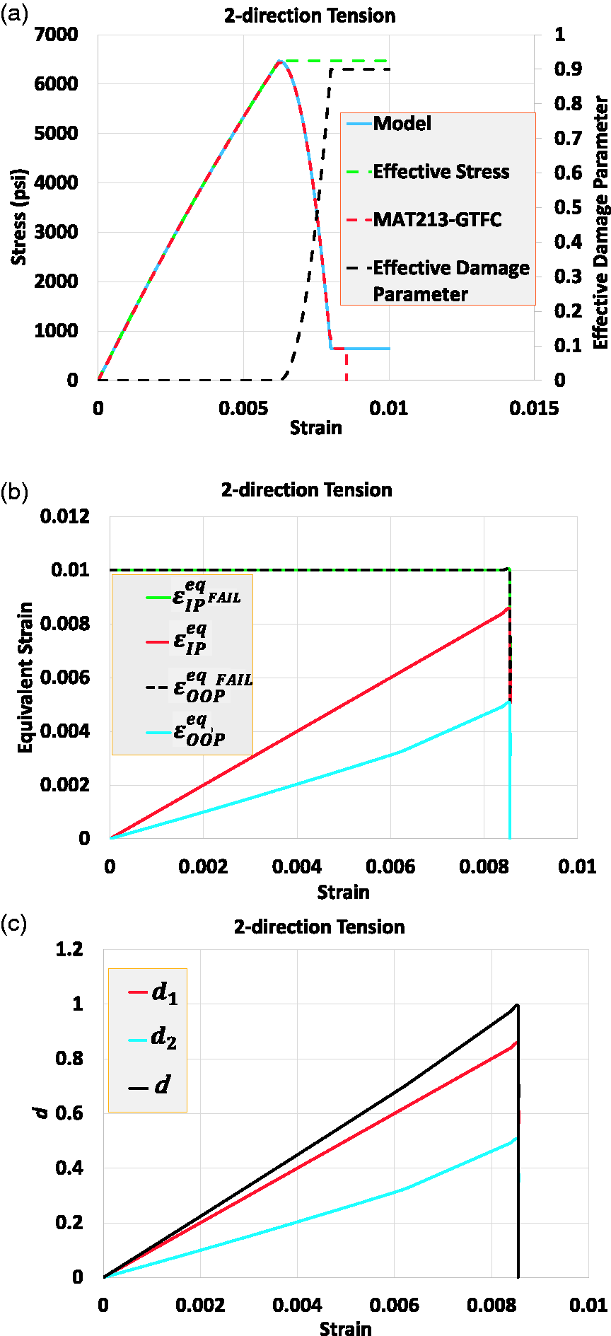
GTFC input and results: 2-direction tension test (a) Stress and effective damage parameter versus strain response (b) Equivalent strain versus strain (c) d, d1 and d2 versus strain.
Results: The drop in the stress value at a strain of ∼0.008 is because of element erosion. Figure 7(b) shows
Discussions: The simulation stress-strain response matches the Model curve in both the pre-peak and the post-peak regimes. As is evident from Figure 7(c), the element is eroded when
Stacked-Ply validation test with PFC and GTFC
Background: The first set of validation tests was done using stacked-ply specimens consisting of 8 plies with a lay-up of [0/90/45/–45]s as shown in Figure 8. Two different tests were carried out – (a) specimen subjected to tension in the y-direction, and (b) specimen subjected to compression in the y-direction. The grey colored regions represent the portion of the specimen which were tabbed using glass fiber tabs and gripped in the test fixture.3,27
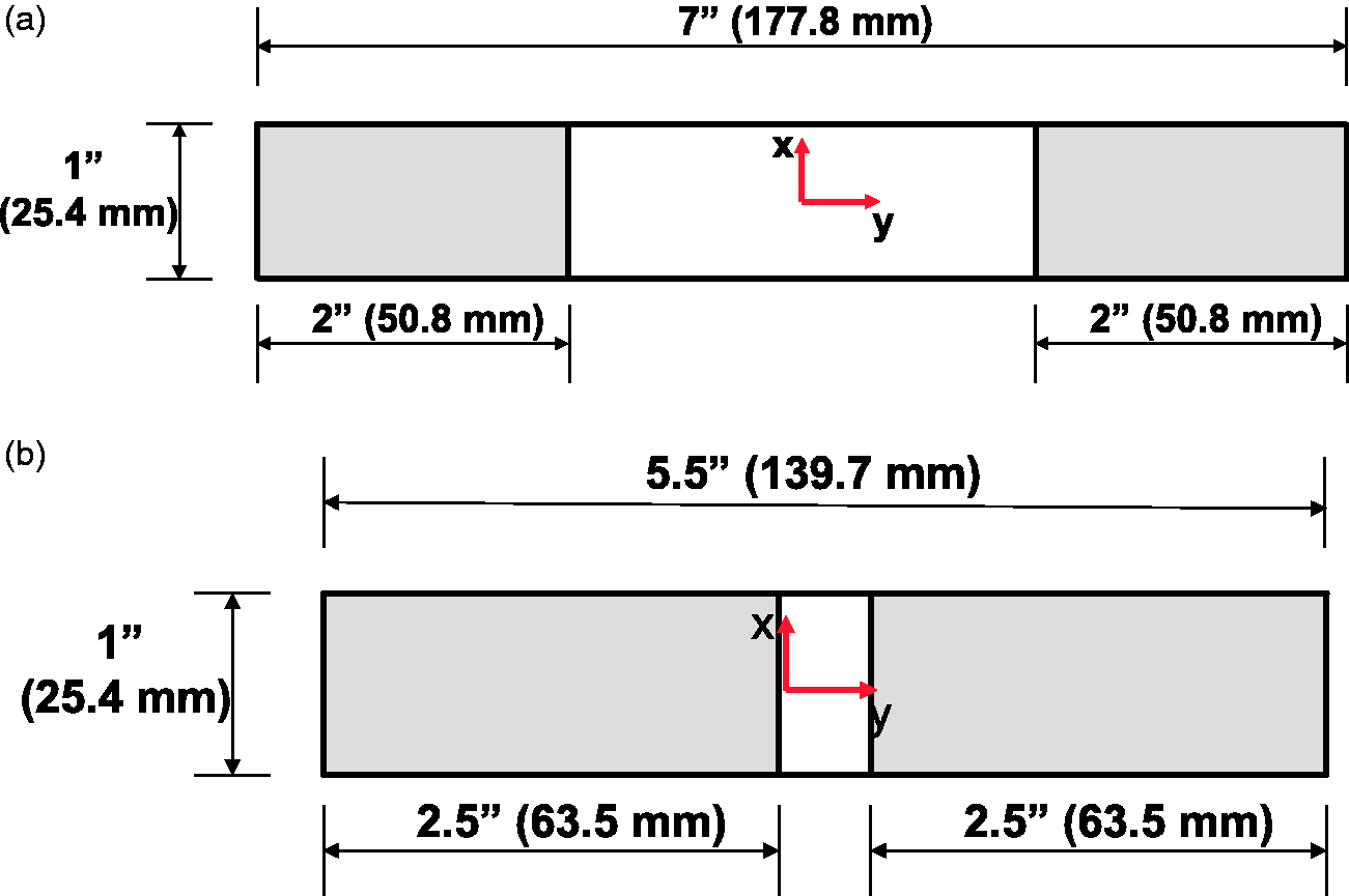
Schematic diagram (a) tension test (b) compression test. 3
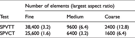
Finite Element Modeling: The tabbed regions in the specimen were excluded from the finite element model to create a computationally efficient model. Figure 9 shows the FE models with the fine mesh used for the stacked-ply validation tension test (SPVTT) and stacked-ply compression validation test (SPVCT). 8-node hexahedral elements were used. There are eight elements through the thickness corresponding to the eight plies in the experimental specimen. Table 2 shows FE model details for the fine, medium and the coarse meshes. The SPVTT boundary conditions are shown in Figure 10 using the highlighted nodes in the fine mesh model. All of the nodes on the support face were restrained from displacement in the y-direction as shown in Figure 10(a). The center line nodes through the z-direction were restrained from displacement in the x-direction as shown in Figure 10(b). This process was done to avoid strain localization on the support face. Since only the gage section is modeled, the displacement at the end of the gage section from the experiment was taken from the Digital Image Correlation (DIC) analysis 27 and applied to the FE model along the positive y-direction on the loading face nodes as shown in Figure 10(c). The nodes on the loading face were also restrained in the x-direction. To avoid rigid body motion in the z-direction (out-of-plane), the center line nodes through the x-direction on either end are restrained in the z-direction direction as shown in Figure 10(d). The boundary conditions are similar for both SPVTT and SPVCT models except for the applied loading. Also, in the case of SPVCT, all the nodes at the support face were restrained in displacements in both the x and the y-directions. LS-DYNA’s 7 reduced integration option has been used with appropriate hourglass control.
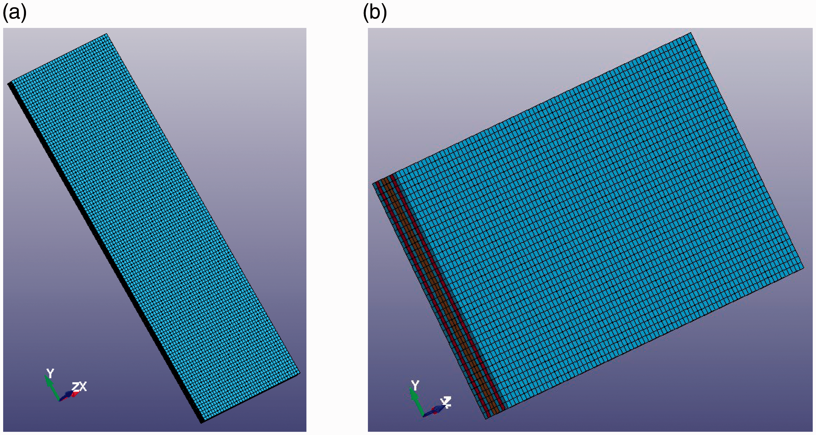
FE model used for (a) stacked-ply validation tension test (SPVTT) (b) stacked-ply validation compression test (SPVCT).
Number of elements in the FE models.
SPVTT boundary conditions (a) y-displacement restraint (b) x-displacement restraint (c) x-displacement restraint and applied displacement along y-direction (d) z-displacement restraint.
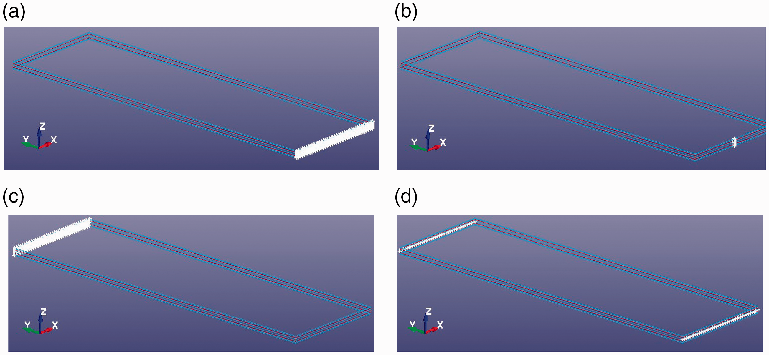
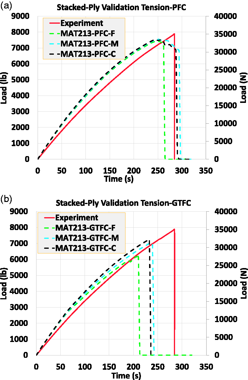
Results: The load versus time graph is used to compare FE and experimental results. For the FE model, the nodal reactions at the support face along the loading direction were added to obtain the load value. The experimental values were obtained from the test frame load cell. The SPVTT load vs time graphs with PFC and GTFC are shown in Figure 11(a) and (b), respectively. The energy vs time graph with the fine mesh is shown in Figure 12.
SPVTT load versus time plot with (a) PFC and (b) GTFC.
SPVTT energy versus time plot (fine mesh model) with (a) PFC and (b) GTFC.
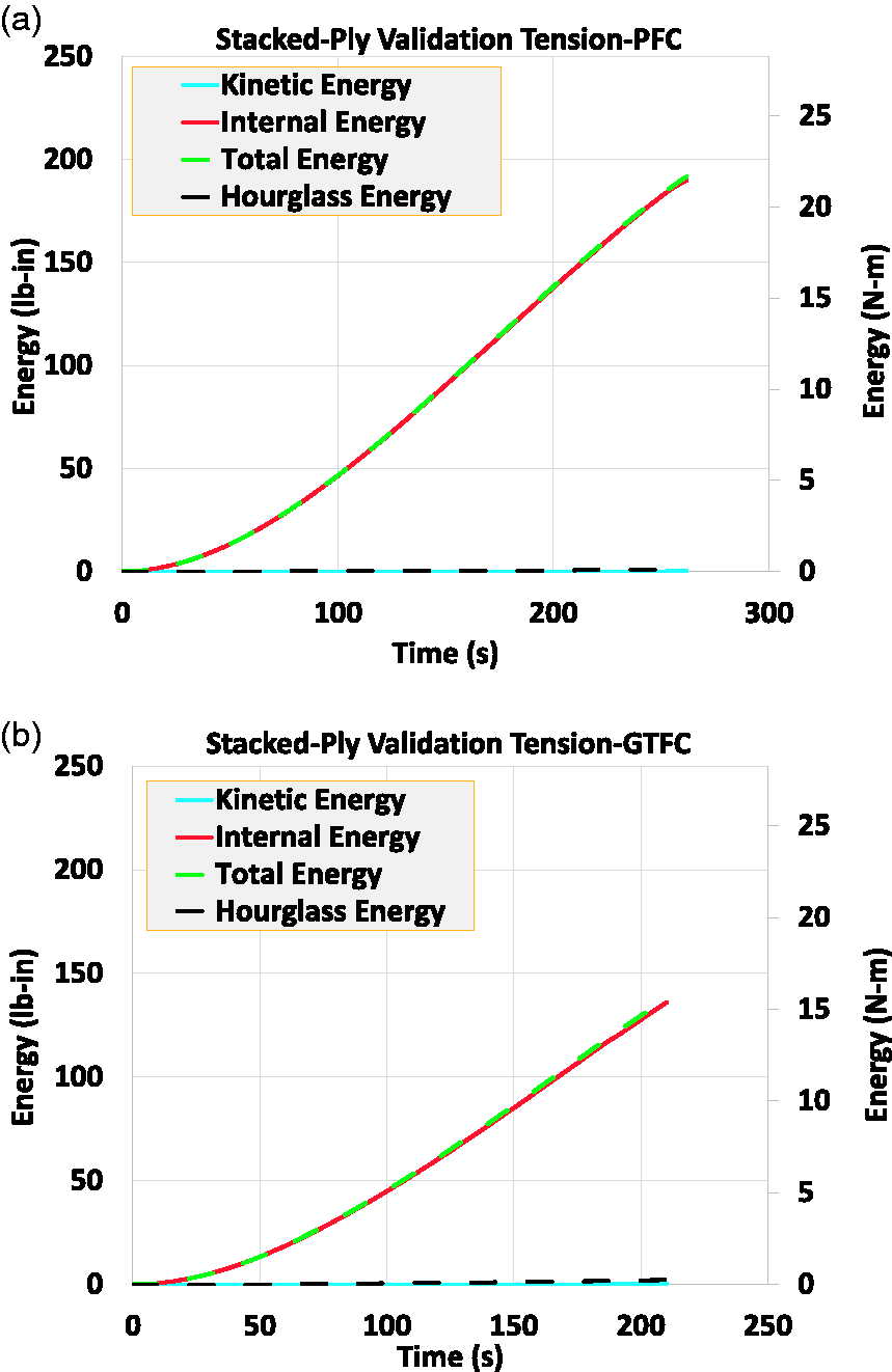
The SPVCT results are shown in Figure 13(a) using PFC with the fine mesh before failure-related parameters were calibrated as well as after calibration. The GTFC results are shown in Figure 13(b). No failure-related parameter calibration was performed. The corresponding energy plots are shown in Figure 14(a) and (b), respectively.
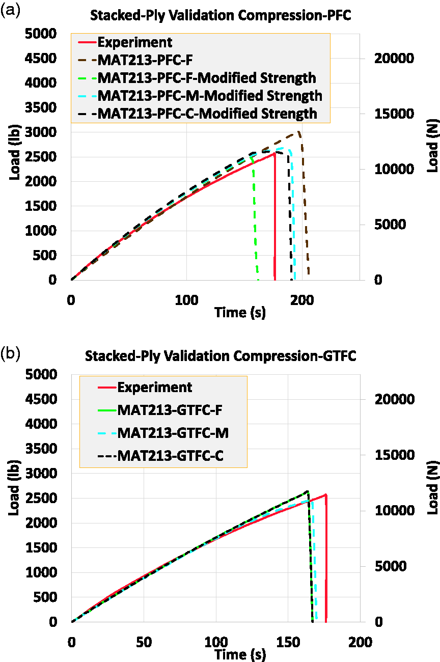
SPVCT load versus time plot with (a) PFC and (b) GTFC.
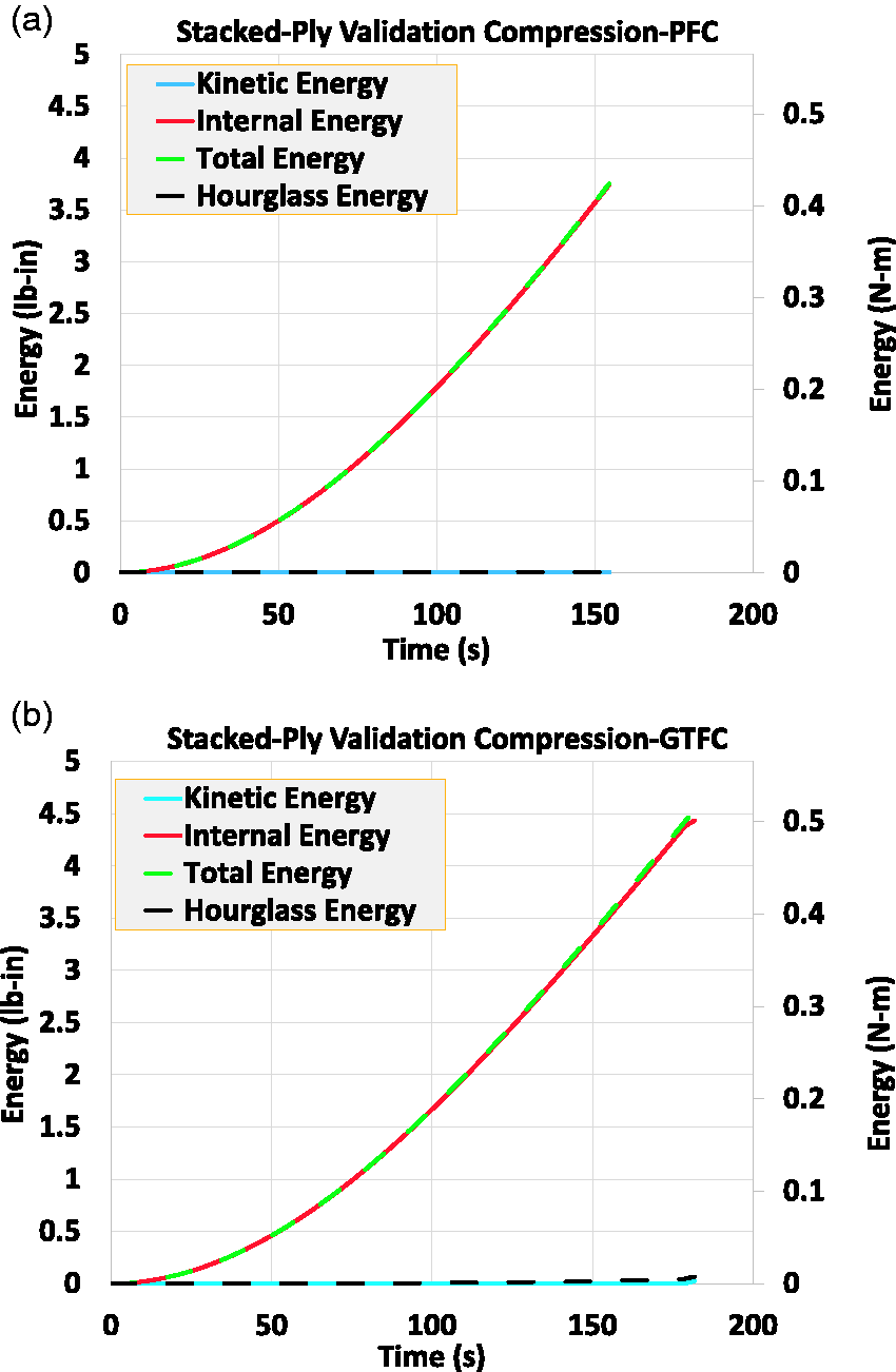
SPVCT energy versus time (fine mesh) with (a) PFC and (b) GTFC.
Discussion SPVTT Models: The peak load predicted using PFC agrees well with the experimental results. The overall FE response is a little stiffer. The distribution of the longitudinal stress (y-stress) is uniform in the model. IFF first initiates in the ±45° plies, then in the 90° plies, after which FF initiates in the 0° plies. This process is immediately followed by a uniform erosion of the elements throughout the entire model. The differences when there is complete loss of load carrying capacity (zero load value) amongst the three mesh sizes is probably due to the different aspect ratios used in these models. The aspect ratios of the element play an important role in element erosion (equation (6)). Overall, the prediction is an improvement compared to results using the earlier implementation of PFC. 3 In the simulations using GTFC, the equivalent failure strain was assumed to be 0.8. The peak load predictions are lower than the experimental values - the coarse and the medium model are about 15% less and the fine model is about 20% less. It should be noted that after the true stress reaches the peak in each component of input stress-strain curves, the true stress starts to degrade. This finding is in contrast to PFC where the true stress degrades only after the failure criterion is satisfied. The difference in the prediction amongst the different mesh sizes (about 5%) can be attributed to the fact that GTFC is not mesh independent.
Discussion SPVCT Models: In the model using the fine mesh with PFC, the peak load prediction was about 20% higher than the experimental result. Subsequently, a few failure-related parameters were calibrated. The 1-direction compressive strength,
In all the stacked-ply simulations, the load is predominantly carried by the 0° plies. As can be seen from the energy plots, as required, the kinetic energy and the hourglass energy are negligibly small for both PFC and GTFC. Some improvements can be made to the models. First, only the gage section of the specimens is modeled. Modeling the whole specimen with the fiberglass tabs will lead to a much larger model but may improve the predictions made for the compression test since boundary effects such as stress concentrations can be avoided. This change will also require the modeling of the interface between the tabs and the composite. In the ±45° plies in the FE model, the edges of the elements are aligned along the loading direction rather than the along the fibers. Modeling the edges of the elements in ±45° plies along the fiber direction with the use of tie-break may improve the results as failure of elements is in this case, dependent on element orientation.
Impact validation test
Background: A set of ballistic impact tests was conducted at NASA-Glenn Research Center. 28 These tests were designed to produce validation test data for the developed MAT_213 constitutive model. In each of the tests, the target is a composite panel impacted with a 50 gm (0.122 lbm) aluminum projectile at different velocities ranging from 119 ft/s (36.3 m/s) to 530 ft/s (161.5 m/s). The composite (flat) panel is made of 16 plies of T800/F3900 composite with a lay-up of [(0/90/45/–45)2]S. The dimensions of each panel are 12 in. x 12 in. x 0.122 in. (30.48 cm x 30.48 cm x 0.3099 cm). DIC data gathered from high-speed cameras were used with the ARAMIS software system28,29 to obtain both projectile information as well as the displacement of the front and back sides of the impacted panel.
In this paper, the LVG1075 test with the projectile velocity as 385 ft/s (117.3 m/s) is chosen for validating the improved failure sub-models. Figure 15(a) shows that the panel is clamped and bolted, and Figure 15(b) shows a close-up view of the rear side of the panel with visible damage. The projectile rebounded after the impact with an average velocity of 46.4 ft/s (14.15 m/s).

(a) Back view of the composite panel after the test clamped (b) Zoomed in picture of the cracks formed on the back side of the panel. 3 Closer examination shows a through crack.
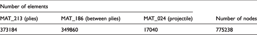
Finite Element Modeling: The FE model is shown in Figure 16. Table 3 shows the details of the FE model. 8-node hexahedral elements were used. The panel is modeled using 16 elements through the thickness with a one-element layer for each ply. In between the plies, cohesive zone elements are used. There are 15 CZE layers modeled using LS-DYNA’s MAT_COHESIVE_GENERAL, 30 also known as MAT_186. MAT_186 can be used for modeling cohesive zone elements with an arbitrary traction-separation law in the form of tabulated data. Interaction between fracture modes I and II is accounted for via a damage formulation. The aluminum projectile was modeled using LS-DYNA’s MAT_PIECEWISE_LINEAR_PLASTICITY, 30 also known as MAT_024. MAT_024 is an elastic-plastic isotropic material model where the yield stress can be scaled as a function of strain rate. The nodes at the location of the bolts are restrained in-plane, and the nodes at the clamps are restrained in the out-of-plane direction.
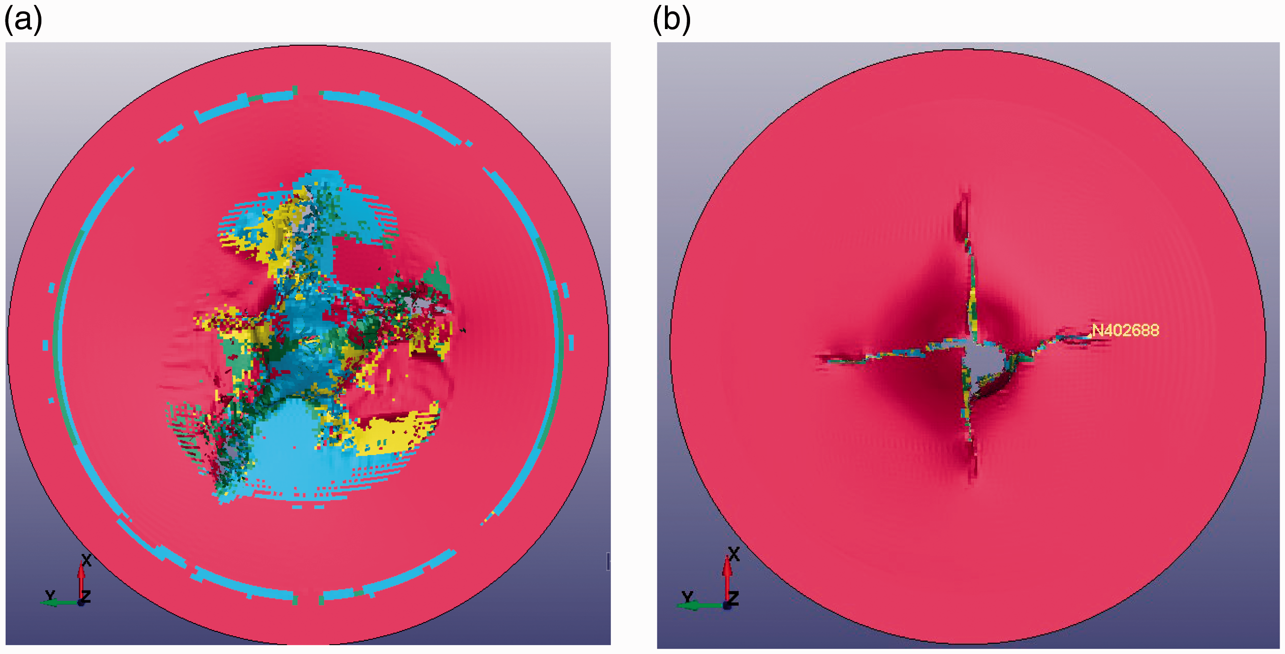
LVG1075 simulation showing impacted panel at the final time step with the projectile hidden from view (a) using PFC (b) using GTFC.
FE model details.
Numerical calibration was used with the PFC model. The post-peak residual damage parameters used were:
Results: Figure 16(a) shows the last frame from the LVG1075 simulation run with PFC and Figure 16(b) with GTFC. The simulations were terminated when the projectile rebound velocity became constant. Node identified as N402688 in Figure 16(b) is used to track and compare the out-of-plane displacement (Figure 17(a)). Figure 17(b) shows the projectile velocity as a function of time. It should be noted that (a) negative velocity indicates projectile rebound, and (b) the average rebound velocity of the projectile obtained from the experiment is shown as an average value.
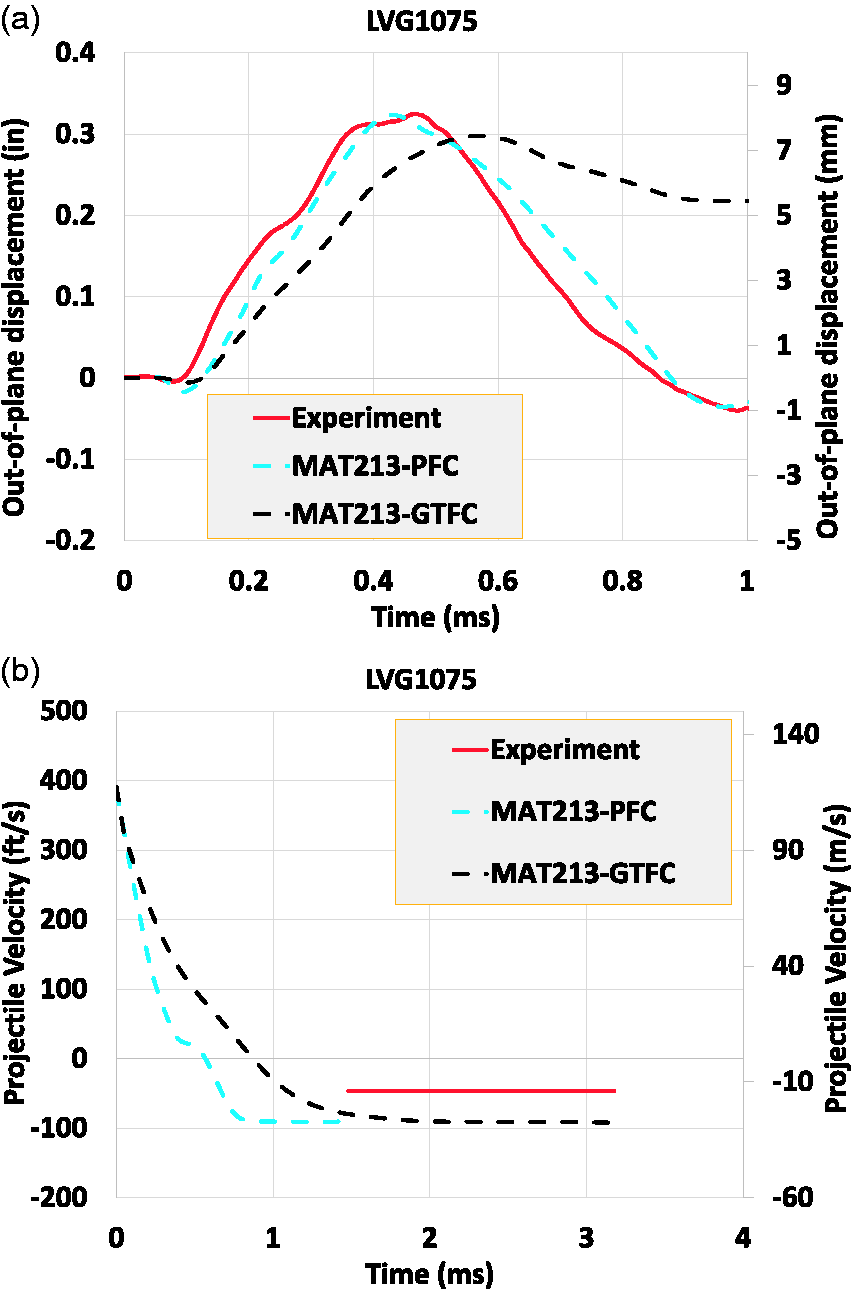
(a) Out-of-plane displacement at node 4,02,688 (b) Projectile velocity plotted against time. Experimental rebound velocity estimated and averaged over a period of 1.5 ms.
Discussions: As can be seen from Figure 16(a), there is widespread surface damage including elements eroded around the clamped region in the FE model contrary to the experimental results (Figure 12). The element erosion is due to the combination of both FF and IFF. The out-of-plane displacement is captured very well for the first 1 ms that includes both the first positive and the first negative peaks. It should be recognized that node 4,02,688 in the region with considerable surface damage starting around 1 ms and hence both the FE computed response and the experimental values are reliable only for that time duration. The calibration of the six failure-related parameters yields a flakier panel with a different damage and crack patterns and a higher rebound velocity. Perhaps, regression analysis involving these parameters may yield improved results, but the primary objective of the validation test is to show the difficulties in modeling impact tests without resorting to an involved parameter calibration process.
The GTFC results show qualitatively that the crack pattern obtained from the FE simulation reasonably matches the experiment. In addition, the crack is a through crack similar to the experiment. The maximum out-of-plane displacement prediction agrees well with the experimentally obtained value though there is difference in the wavelength of the displacement profile. The rebound velocity it overestimated similar to the PFC results. It should be noted that the calibration of the input residual strength was done with multiple objectives – matching crack pattern, out-of-plane displacement and rebound velocity, and it is very likely that decreasing the residual strengths in the tension and the shear components can lead to a less stiff panel response.
Concluding remarks
A three-dimensional general orthotropic material model involving elastic and inelastic deformations, damage and failure has been presented. The focus is on handling the challenges of a continuum level model in predicting when failure would take place in two loading scenarios - quasi-static loading, and high velocity impact events. Improvements were made to the post-peak behavior of the Puck Failure Criterion. These changes resulted in much better prediction for the staked-ply tension and compression validation tests. Minor calibration was needed to improve the results for the stacked-ply compressive test. Linking the post-peak behavior to fracture energy makes the strength predictions less dependent on the finite element mesh as evidenced from the convergence analyses. The impact test simulation required calibration of the post-peak residual damage parameters to obtain a reasonable prediction. The out-of-plane displacement is predicted very well for the first 1 ms following the impact. The rebound velocity is within 10% of the experimental result after normalization with respect to impact velocity. However, the damage and crack patterns are different. The material behavior appears to be flaky in comparison to the tested composite panel.
The Generalized Tabulated Failure Criterion is a new failure criterion implemented in MAT_213. It permits an arbitrary-shaped failure surface to be defined and used. In its current form, the failure surface is decomposed into in-plane and out-of-plane failure modes thereby making it suitable for modeling unidirectional composites. The stacked-ply tension test results show the peak load to be underpredicted, but the compressive test results are very close to the experimental results. Minimal calibration was done with the residual strength and failure strain values. The strength of GTFC is demonstrated in the impact test simulation. The rebound velocity is within 10% of the experimental result after being normalized with the impact velocity. The crack pattern qualitatively matches the experimental results. The out-of-plane displacement is close to the first positive peak, but appears to diverge from the experimental results after that.
It is well understood that damage and failure of composite systems is driven by the composite architecture and the constituent materials, and that while multi-scale modeling may make the numerical model more predictive, the enormous computational expense makes this approach untenable. What is desirable from an analyst’s viewpoint, is a reasonable and systematic approach that requires (a) input data that is largely experimental (physical and virtual) driven, (b) a small number of damage and failure-related parameters, and (c) an even smaller number of parameters that may require some tuning/calibration to yield consistent and somewhat conservative results. Further improvements that can be made to make the predictions more accurate include (a) using rate-dependent stress-strain data in the deformation sub-model, (b) making damage and failure rate-dependent, and (c) defining a richer failure surface for use in GTFC. Analysis of the impact FE simulations show that the computed strain-rate values are very high (in the order of 103). There is ample experimental evidence showing that for unidirectional carbon/epoxy composites the strength in the in-plane shear and the transverse components increase with increase in strain-rate. 31 These issues are being addressed in ongoing research work.
Footnotes
Declaration of Conflicting Interests
The author(s) declared no potential conflicts of interest with respect to the research, authorship, and/or publication of this article.
Funding
The author(s) disclosed receipt of the following financial support for the research, authorship, and/or publication of this article: Authors Shyamsunder, Khaled, and Rajan gratefully acknowledge the support of the Federal Aviation Administration through Grant #12-G-001 titled “Composite Material Model for Impact Analysis” and #17-G-005 titled “Enhancing the Capabilities of MAT213 for Impact Analysis”, William Emmerling and Dan Cordasco, Technical Monitors.