






Abstract
By analyzing 3,094 U.S. counties from 2015 to 2019, this study examines spatial spillover effects of state policy environments on county-level mortality rates. I developed a weighted spatial difference score that captures relative policy contrasts between neighboring states and geographic proximity to borders. Consistent with prior studies, more liberal state policies are associated with significantly lower mortality rates. After considering spatial spillovers, I found that counties experience cross-border spillovers based on policy differences with neighbors: Those bordering states with relatively more liberal policies showed lower mortality than their own policies predict, while those bordering states with relatively more conservative policies showed higher mortality (11.8 additional deaths per 100,000 per 1 SD of policy contrast). Importantly, conventional models ignoring spatial spillovers underestimated direct policy effects by 24.8%, systematically undervaluing policy interventions’ true health returns.
Introduction
Over recent decades, scholars have demonstrated that health outcomes are shaped not only by individual-level factors but also by broader contextual environments that create conditions for health and illness. Among these contextual factors, state policies have emerged as particularly influential due to the unique federal structure of the United States, which grants states substantial autonomy in enacting and implementing laws and policies even when these diverge from federal measures (Bambra, Smith, and Pearce 2019). The significance of state policy environments has grown more pronounced as states have become increasingly polarized along the liberal–conservative continuum over the past three decades (Montez and Grumbach 2023). Existing literature consistently shows that liberal state policies, including higher minimum wages, comprehensive parental leave programs, stricter firearm regulations, substance abuse prevention measures, and more generous welfare programs, are associated with better health outcomes and behaviors (Kemp, Grumbach, and Montez 2022; Sun 2025; VanHeuvelen, Wang, and VanHeuvelen 2024).
However, previous studies typically treat states as isolated geographical units, overlooking the reality that state boundaries are permeable to policy effects. This oversight is particularly significant given that approximately one-third of the U.S. population (33.7%) resides in counties that border other states (author’s calculation). For these residents, state boundaries often represent administrative rather than practical barriers given that people regularly cross borders to access employment, commodities, health care, and other resources unavailable in their home states. Research across multiple policy domains demonstrates substantial cross-border responsiveness, from workers commuting to higher wage jurisdictions to patients seeking specialized medical care, with effects declining systematically as distance from state borders increases (Agrawal 2015; Baker, Johnson, and Kueng 2021; Glass et al. 2022; Jardim et al. 2024; Lovenheim 2008). That means state policy effects frequently transcend administrative boundaries through various spillover mechanisms, including economic linkages, shared media markets, and social networks that span state lines (Li 2014). Without accounting for these geographic patterns and potential cross-border dynamics, traditional analyses may misestimate the full impact of state policies on population health outcomes.
This study addresses this gap by examining whether and how the health impacts of state policies extend beyond their borders, investigating spatial spillover effects in county-level mortality rates across the liberal–conservative policy continuum. Using a novel measurement called the “weighted spatial difference score,” the current study captures both policy contrasts between counties in neighboring states and their varying influence based on each county’s geographic distance from state borders. This approach provides a more nuanced understanding of state policy exposure because it quantifies both the magnitude and geographic reach of policy discontinuities. By incorporating these spatial dimensions into county-level mortality analysis, it highlights how state policy effects ripple across administrative boundaries and where geographic location might amplify or attenuate these effects.
Background
U.S. State Policy Environments and Population Health
Recent studies on population health in the United States have highlighted the importance of macro-level contexts and upstream factors in shaping the distribution of downstream social determinants of health (Ray, Lantz, and Williams 2023). This approach criticizes explanations focusing on actions and choices made by individuals without contextualizing risk factors that “put people at risk of risks” (Link and Phelan 1995:81). This means that understanding health outcomes requires examining broader social, economic, and political structures that create conditions where certain populations become more vulnerable to adverse health outcomes. When only considering individual-level determinants of health outcomes, researchers may neglect the social settings that fundamentally shape individual choices, behaviors, and access to health-promoting resources through institutional arrangements and policy environments (Hummer and Hamilton 2019). For instance, the mortality risk of low-educated populations has changed dramatically with the change in state environments, although that of highly educated populations declined to similar levels across most states (Montez, Zajacova, et al. 2019). This pattern demonstrates how state-level contextual factors can amplify or mitigate health disparities by disproportionately affecting certain populations who have fewer resources to buffer against adverse contextual environments.
While there is no clear consensus about how to define the boundaries of “macro-level” (Chen and Gotway Crawford 2012), empirical evidence consistently demonstrates the crucial role of state contexts in the United States. (Bambra et al. 2019; Kemp et al. 2022; Montez, Hayward, and Zajacova 2019). The significance of U.S. states stems from the unique political structure of the U.S. federal system, which grants states substantial policymaking authority that can operate even when it diverges from federal legislation. Indeed, over the past few decades, U.S. states have emerged as increasingly autonomous policymaking entities (Grumbach 2018). What makes this unique political setting in the United States more important is that the influence on population health is not limited to health-related supply-side policies like health care infrastructure, insurance coverage, and provider availability. Rather, the effects extend to a broader range of state policies affecting social and economic conditions, including labor market regulations, environmental protections, and social welfare programs that shape population health through multiple pathways (Hummer and Hamilton 2019; McFarland, Hill, and Montez 2023). For instance, research has shown that a 10% increase in minimum wage reduces non-drug suicides among low-educated adults by 2.7 %, while a comparable increase in Earned Income Tax Credit results in a 3.0 % reduction. Similarly, $1 increases in minimum wages are associated with 1.4 percentage point decreases in smoking prevalence (Leigh, Leigh, and Du 2019).
A growing number of studies examine the impact of multiple state policies on population health. Instead of investigating the impact of one specific health-related policy, these studies consider the fact that many state policies are enacted or disappear as a “bundle” (Montez and Grumbach 2023; Pacheco and LaCombe 2022). One consistent finding from those studies is that liberal state policies, including higher minimum wages, stronger environmental regulations, more generous social welfare benefits, comprehensive public health programs, and expanded health care access, are associated with lower mortality rates and less risky health behaviors (Montez, Hayward, and Zajacova 2021). In a series of studies, Montez emphasized that state policy contexts in the United States have become increasingly polarized over the past few decades, with consequences that are likely to cement diverging trajectories in states’ democratic performance and population health outcomes (Montez and Grumbach 2023). Using a policy liberalism index spanning 16 policy domains created by Grumbach (2018), Montez et al. (2022) demonstrated that shifts in states’ liberal–conservative policy orientation significantly predict variations in working-age mortality rates. Their analysis revealed substantial potential impacts of policy orientation on population health: Adopting fully liberal policies across all states could have prevented 171,030 deaths in 2019, while implementing fully conservative policies might have resulted in 217,635 additional deaths. Similarly, one recent study found that right-leaning and right-moving states tend to be consolidating risky health behaviors over the past 30-year period (VanHeuvelen et al. 2024).
Taken together, this body of evidence establishes a robust association between state policy liberalism and population health outcomes. The present study builds on this foundation by first replicating this association in the current sample before extending the analysis to examine whether and how policy effects cross state boundaries.
It should be noted that beyond replicating this established association, Hypothesis 1 serves as a necessary analytic baseline: By comparing the policy liberalism coefficient in models that omit versus include the weighted spatial difference score, the analysis quantifies the degree to which conventional aspatial models underestimate the true direct effects of state policies on population health. This connection between Hypothesis 1 and the study’s central methodological contribution is elaborated in the section on analytic strategy.
Spatial Dynamics of Health Determinants
While existing research demonstrates that liberal state policies associate with better health outcomes, these studies typically employ aspatial analytical frameworks that may underestimate policy impacts. By treating states as isolated units, conventional approaches overlook how policy effects operate across administrative boundaries through population mobility, economic integration, and resource sharing. To address this, previous spatial approaches to population health recognize that individuals’ health outcomes reflect exposures beyond their immediate residential jurisdictions (Yang, Noah, and Shoff 2015). This perspective challenges the assumption of spatial independence, the notion that health determinants in one area operate independently of conditions in neighboring areas. In reality, adjacent jurisdictions often exhibit correlated health outcomes due to shared socioeconomic characteristics, environmental conditions, population mobility, and policy diffusion across boundaries (Tabb et al. 2018). Indeed, studies increasingly incorporate spatial interdependence into analytical models, demonstrating that neglecting spatial autocorrelation can produce misleading estimates of contextual effects (Sparks and Sparks 2010; Ulimwengu and Kibonge 2021; Yang et al. 2015). For instance, beyond direct within-county effects, simultaneous socioeconomic improvements across all contiguous counties would reduce a typical county’s diabetes mortality rate by approximately 29% (Turi and Grigsby-Toussaint 2017).
The concept of “spatial polygamy” (Matthews and Yang 2013) offers one useful lens for understanding how state policy effects transcend administrative boundaries. Spatial polygamy refers to individuals’ simultaneous exposure to multiple geographic contexts through daily activities that span jurisdictional boundaries. Rather than being exclusively influenced by their residential location, people traverse multiple policy environments through employment, shopping, health care seeking, and social interactions. This phenomenon is particularly pronounced in border regions, where residents can easily access resources, services, and opportunities in neighboring states with different policy regimes. For example, COVID-19 mobility restrictions achieved only 54% effectiveness at the county level compared to statewide policies, as residents traveled to less restricted neighboring counties, while stay-at-home orders reduced mobility by 30% to 50% in adjacent nonrestricted counties through both physical movement and information spillovers via shared media markets (Chang et al. 2023; Elenev et al. 2021).
Cross-border economic and social integration creates systematic patterns of resource access that vary with proximity to state borders. People regularly cross state lines to access lower sales tax rates, higher wage employment opportunities, prescription medications under different regulatory regimes, and specific health care services unavailable or less accessible in their home states (Baker et al. 2021; Glass et al. 2022). Empirical evidence across multiple policy domains demonstrates substantial cross-border responsiveness to policy differentials. For instance, local sales tax rates on the low tax side of state borders are 1.25 percentage points higher than interior communities, reducing state tax differentials by over three-quarters, with effects declining systematically as driving time from borders increases (Agrawal 2015). These patterns demonstrate that policies influence behaviors and outcomes well beyond their jurisdictional boundaries, with effects diminishing as distance from policy discontinuities increases.
These cross-border dynamics have direct implications for population health outcomes in border counties. When residents of a county in a relatively conservative state border a more liberal neighboring state, they gain access to that neighbor’s more generous health care infrastructure, stronger workplace protections, higher minimum wages, and more comprehensive public health programs through commuting to higher wage jobs, seeking care across state lines, and exposure to health-promoting norms via shared media markets and social networks. Conversely, counties in liberal states bordering more conservative neighbors may experience negative spillovers as residents access fewer health-protective resources in adjacent jurisdictions. These spillover effects should decline with geographic distance from state borders as cross-border access costs increase and cross-state integration weakens. This spatial structure of policy exposure suggests that conventional models examining only within-state policy effects systematically misestimate the true impacts of state policy environments (Harding, Leibtag, and Lovenheim 2012; Jardim et al. 2024).
State policy spillovers may operate through numerous mechanisms. This study tests two potential pathways through which cross-border policy contrasts may influence mortality: health behavior diffusion and health care supply spillovers. Health behavior diffusion occurs when policy-induced norms, practices, and behaviors diffuse across state boundaries through social networks, shared media markets, and cross-border interactions. Social network research demonstrates that health behaviors spread through existing connections via mechanisms including normative influence, behavioral modeling, and social reinforcement (Chiu and West 2007). Since social networks are not constrained by administrative boundaries, policy-driven behavioral changes may propagate across state lines. Recent evidence on nicotine vaping restrictions illustrates such patterns: Neighboring counties experienced 14% to 79% increases in product sales following restrictions (Cheng, Liber, and Levy 2024), while emergency bans during the 2019 e-cigarette or vaping product use-associated lung injury outbreak generated a 94.5% increase in refill sales in border counties (Chen, Jiang, and Prakash 2024). Similarly, research on cigarette taxation reveals that 13% to 25% of consumers purchase cigarettes in border localities, with demand elasticity varying significantly by distance to lower-price borders (Lovenheim 2008).
If health behavior diffusion represents a meaningful spillover mechanism, counties bordering more liberal states should exhibit healthier behavioral profiles independent of health care access. Liberal state policies typically include comprehensive tobacco control measures, stricter alcohol regulations, and robust public health campaigns promoting healthy lifestyles. These policy-driven health norms may diffuse into neighboring counties through shared media markets spanning state boundaries, cross-border social networks, and workplace environments where employees from multiple states interact daily, creating unique exposure patterns whereby residents’ health outcomes reflect both their own state’s policies and neighboring states’ resources. For instance, a county in a conservative state bordering a liberal state with aggressive anti-smoking campaigns might experience reduced smoking prevalence through shared media exposure and observation of lower smoking rates among cross-border contacts. Conversely, counties bordering more conservative states may experience negative behavioral diffusion, adopting less healthy norms prevalent in adjacent jurisdictions.
Health care supply spillovers, by contrast, occur when residents directly access medical services across state lines, benefiting from neighboring states’ health care infrastructure, provider availability, and service accessibility shaped by different policy environments. For example, Li (2014) found that county mortality is influenced not only by in-state physicians but also by out-of-state physicians practicing near border counties. Other research suggests that health care supply in some counties is constrained by policies in neighboring states. Horwitz and Polsky (2015) demonstrated that border counties regulated by Certificate of Need measures averaged 6.4 fewer magnetic resonance imaging units per million population when adjacent to unregulated states. To seek needed health care, people actively travel across the state borders. For instance, abortion access research reveals substantial cross-state health care mobility, with an average of 8% of patients traveling across state lines in 2017, reaching 74% in states with restrictive policies and limited facilities (Smith et al. 2022). These patterns reveal how policy differences create systematic disparities in health outcomes, particularly in border regions where geographic proximity does not guarantee equal access to care or equal exposure to health-protective regulations.
If health care supply represents a potential spillover mechanism, policy contrasts with neighboring states should directly influence health care provider availability in counties near the border. Liberal state policies typically generate more robust health care infrastructure through Medicaid expansion, higher provider reimbursement rates, stronger support for community health centers, and more generous mental health funding. Consequently, state policies may exhibit attenuated associations with health outcomes in border counties as residents partially substitute neighboring states’ resources for those constrained by their home state’s policies (Horwitz and Polsky 2015). These policy investments create regional provider concentrations benefiting both liberal state residents and individuals in adjacent counties who cross state lines for care. For example, a county in a conservative state without Medicaid expansion bordering a liberal state with expanded Medicaid might exhibit higher effective provider availability as residents travel across borders for care and providers locate strategically near borders to serve populations from both states. This mechanism would manifest as higher health care provider rates in counties bordering more liberal states, even after controlling for the focal county’s own state policies and demographic characteristics.
Data and Methods
Weighted Spatial Difference Score
Spatial analytical approaches have become increasingly sophisticated in health research, enabling researchers to account for geographic interdependence in policy effects. Conventional spatial econometric models construct “spatial weights matrices” that quantify geographic relationships between units based on shared borders, addressing different forms of spatial interdependence through spatial lag of independent variable, or spatial Durbin specifications (Grubesic and Rosso 2014; Yang et al. 2015). When the key independent variable is measured at the state level, however, these spatial models are poorly suited for capturing cross-border policy dynamics.
Conventional spatial models use neighbors’ policy positions rather than policy contrasts as the key predictor. Figure 1a illustrates z-standardized policy liberalism scores of Texas and its four neighboring states. County A received a spatially lagged value of .79 (reflecting New Mexico’s liberal policies), while County B received −.90 (reflecting Oklahoma’s conservative policies). This approach misses what matters theoretically: the size of the policy gap between a county and its neighbor. Texas had a policy liberalism score of −.80. County A borders New Mexico (.79), creating a policy contrast of 1.59 SD (−.80 − .79 = –1.59), generating strong incentives for residents to cross state lines for better health care, higher wages, and stronger protections. County B borders Oklahoma (−.90), producing a minimal contrast of only .10 SD, offering relatively few reasons for cross-border movement. Because standard spatial Durbin or spatial lag models use neighbors’ raw policy scores rather than the gap between a county and its neighbor, they cannot directly capture the policy discontinuity that motivates cross-border movement. As a result, these models conflate two different questions: Does living adjacent to a liberal or conservative state matter, or does having a large policy gap with your neighbor matter? The spillover mechanism relevant to border counties operates through the second pathway, through policy discontinuities that create cross-border opportunities.
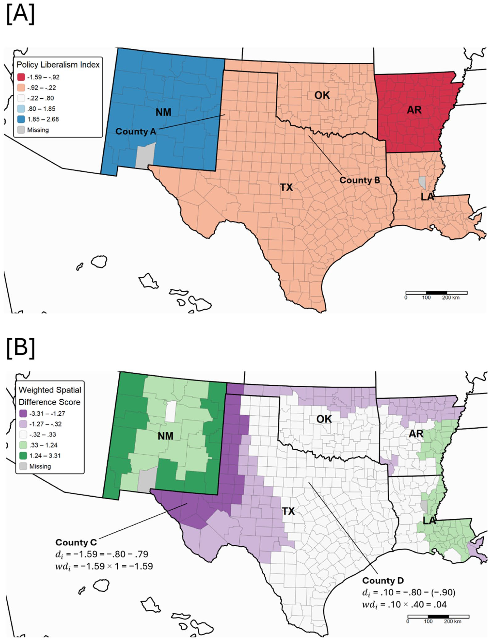
Conceptual map of five states (NM, TX, OK, AR, and LA). (a) Policy liberalism index. (b) Weighted spatial difference score.
Furthermore, spatial models relying on boundary contiguity matrices assign zero border-related exposure to interior counties regardless of their geographic distance from state boundaries. Counties immediately adjacent to border counties receive no border-related exposure at all in standard models even though residents in these near-border interior counties can often access neighboring states almost as easily as border county residents themselves. This omission is particularly consequential in a county-state data structure like the present study, where the key independent variable is measured at the state level. In such a structure, all counties within a state share an identical policy score, making it impossible to capture any gradient of cross-border exposure. A county 20 km from a state border and one 150 km away receive not only the same zero spillover exposure from neighboring states but also the same home state policy score, entirely obscuring the geographic variation in cross-border access that should theoretically shape health outcomes.
To overcome the distance problem, some geography research has incorporated distance decay functions into spatial econometric models to weight nearby neighbors or certain facilities more heavily than distant ones (Elhorst et al. 2024; Wang, Wang, and Onega 2021). This approach has a long tradition in geography through gravity models and potential measures that weight spatial access by distance (Hansen 1959). Typically, these studies define catchment areas using fixed distance thresholds or travel time zones from a focal point (e.g., all hospitals within 30 miles or all employment opportunities within a 60-minute commute). Similarly, border effects studies examining tax avoidance, cigarette purchasing, and minimum wage spillovers have documented that policy responsiveness declines with distance from state borders, with effects measured through discrete distance bands or driving time thresholds (Agrawal 2015; Jardim et al. 2024; Lovenheim 2008). However, these approaches still fail to parameterize the cross-border discontinuity. A Texas county 50 km from the New Mexico border (high policy contrast) receives the same distance weight as a Texas county 50 km from the Oklahoma border (minimal policy contrast). Conventional distance decay models reduce the influence of neighbors with distance, but the weighted value still reflects the neighbor’s absolute policy position rather than the policy gap between the focal county and its neighbor. Treating an absolute policy value as a proxy for spillover potential ignores the true driver of cross-border mobility, which is the magnitude of the policy discontinuity.
Moreover, recent methodological developments have extended difference-in-differences (DiD) frameworks to incorporate spatial dimensions, estimating both direct treatment effects and spillover effects while relaxing the stable unit treatment value assumption that treatment in one unit does not affect outcomes in other units (Butts 2023; Delgado and Florax 2015). However, most spatial DiD implementations employ binary treatment indicators classifying units as either adopting or not adopting a specific policy, such as whether counties ban smoking or states expand Medicaid. This binary approach cannot capture variation in the degree of policy difference between neighboring units, which is precisely what drives cross-border spillover potential in a comprehensive policy environment. This limitation is critical because policies are enacted and abolished as bundles rather than in isolation (Montez and Grumbach 2023; Pacheco and LaCombe 2022). When Texas borders New Mexico, the relevant spillover exposure is the cumulative difference in comprehensive policy orientation across multiple domains, not whether any single policy has been adopted. Binary specifications cannot estimate dose–response relationships showing whether larger policy contrasts generate proportionally stronger spillovers.
To address these limitations, I developed a weighted spatial difference score that overcomes each shortcoming of existing spatial approaches. First, it measured policy contrast directly rather than neighbors’ policy positions. The score quantified both the direction and magnitude of policy differences between a county’s own state and neighboring states. This operationalization isolated the spillover mechanism driven by policy discontinuities rather than conflating it with neighbors’ absolute policy liberalism level. Second, it incorporated distance decay into policy contrast measurement. The score weighted each county’s policy contrast by its geographic distance from state borders using an inverse distance weight function. Third, it used a continuous policy liberalism index spanning multiple domains rather than binary treatment indicators. This captured how comprehensive policy environments varied in degree along the liberal–conservative spectrum, enabling estimation of dose–response relationships between policy contrast magnitude and health outcomes.
Study Sample
To examine the associations between policy liberalism index and age-adjusted mortality rate and their dynamics in and out of border counties, this study combined multiple county-level data sources. For the mortality, the restricted use version of the National Vital Statistics System death certificate files from the National Center for Health Statistics (2021) was used. These data represent a complete census of deaths in the United States, containing detailed information from death certificates filed in all 50 states and the District of Columbia. Each death record includes the decedent’s county of residence, age at death, underlying and contributing causes of death (coded using the International Classification of Diseases, 10th Revision), and demographic characteristics. For the state-level policy liberalism index by Caughey and Warshaw (2016), the most updated version of State Policy & Politics Database (version 1.3) was used. To include demographic and health-related variables, American Community Survey (ACS; U.S. Census Bureau 2020) five-year estimates and County Health Rankings & Roadmaps (CHR; University of Wisconsin Population Health Institute) were used. All measures were calculated as five-year pooled averages to provide more stable estimates and reduce the influence of year-to-year fluctuations. Alaska and Hawaii were excluded from the analysis because these states have no land borders with other states, making the weighted spatial difference score undefined for their counties. After excluding counties with missing values, the final sample size was 3,094.
Dependent Variable
To test Hypotheses 1 to 3, I used the age-adjusted mortality rate over the period from 2015 to 2019. It was calculated for each county using deaths from all causes (all-cause mortality). To account for varying age distributions across counties that could confound mortality comparisons, rates were first calculated for 10-year age groups (0–14, 15–24, 25–34, 35–44, 45–54, 55–64, 65–74, 75–84, and 85+ years) and then age-adjusted using the direct standardization method with the 2000 U.S. standard population weights.
To test mechanisms underlying spatial spillover effects (Hypotheses 3a and 3b), I used several health behavior and health care supply measures. For each variable, I used data from CHR releases (University of Wisconsin Population Health Institute) that corresponded to actual measurement years overlapping with the mortality period between 2015 and 2019. Health behavior measures (smoking, excessive drinking, obesity) were modeled county-level estimates derived by Centers for Disease Control and Prevention (CDC) from the Behavioral Risk Factor Surveillance System (BRFSS) using multilevel modeling approaches. Health care supply measures (primary care physicians, dentists, mental health providers) were derived from the Health Resources and Services Administration (2020) Area Health Resource File and the Centers for Medicare & Medicaid Services (2020) National Provider Identification data.
For health behaviors (Hypothesis 3a), I examined (1) adult smoking prevalence, measured as the percentage of adults ages 18 and older who currently smoke; (2) excessive drinking prevalence, measured as the percentage of adults reporting binge drinking or heavy drinking; and (3) adult obesity prevalence, measured as the percentage of adults ages 20 and older with body mass index ≥30 kg/m2. For health care supply (Hypothesis 3b), I examined provider availability, measured as (1) primary care physicians per 100,000 population, defined as practicing physicians specializing in general practice, family medicine, internal medicine, or pediatrics; (2) dentists per 100,000 population, including all professionally active dentists; and (3) mental health providers per 100,000 population. For data source and years of data, see Appendix Table 1 in the online version of the article.
Independent Variables
The primary independent variable was the state policy liberalism index developed by Caughey and Warshaw (2016), which captured the overall ideological orientation of state policy environments across multiple domains. This validated measure has been widely used in prior research examining state policy effects on population health (Montez et al. 2022; VanHeuvelen et al. 2024). I used the 2014 value of this index, which most directly precedes the mortality outcomes measured from 2015 to 2019, ensuring temporal precedence. The index was z-standardized for interpretation, with higher values indicating more liberal policy environments.
The second independent variable was state border status. Using a spatial weight matrix to identify county adjacencies, I classified counties into border counties (n = 1,129) that share boundaries with other states and non-border counties (n = 1,965) that are completely surrounded by counties within the same state. This binary classification helped identify counties that may have experienced unique policy dynamics due to their location at state boundaries.
The third independent variable was the weighted spatial difference score of the state policy liberalism index. As mentioned previously, this continuous measure quantified each county’s exposure to cross-state policy contrasts, incorporating both the magnitude of policy differences with neighboring states and the county’s distance from state borders. The calculation of the weighted spatial difference score proceeded in two steps.
Step 1 calculated each county’s policy difference score by comparing its own score of state policy liberalism index to those of adjacent neighbor:

where
Step 2 applied a distance weight to these spatial difference scores based on proximity to the nearest state border:

where
Figure 1b visualizes the weighted spatial difference score. For instance, County C is a border county directly on the Texas–New Mexico boundary. The policy liberalism index of Texas and New Mexico was −.80 and .79, respectively. Therefore, the spatial difference score before weighting was −1.59 (−.80 − .79), and since County C is directly on the border (distance = 0), the weight equaled 1, resulting in a final weighted spatial difference score of −1.59. By contrast, County D is not directly on the border but located inland from the Texas–Oklahoma boundary. Given the policy liberalism indices of Texas (–.80) and Oklahoma (–.90), the initial difference score was .10 (−.80 – −.90). Since County D is located approximately 129 km from the nearest border county, its weight is .40 (52 / 129), resulting in a final weighted spatial difference score of .04 (.40 × .10). See Appendix Figure 1, available in the online version of the article, for U.S. maps of original policy liberalism index and weighted spatial difference score and Appendix Figure 2, available in the online version of the article, for the distribution of weighted spatial difference score.
This two-step measurement approach offered several advantages. By capturing the maximum policy difference between neighboring states and weighting it by geographic distance, it identified both the sharpest policy discontinuities and their spatially varying relevance. This measure leveraged the fact that state policies were constant within states but could change abruptly at borders, allowing examination of how exposure to contrasting policy environments may affect mortality rates in border regions. Importantly, this approach generated a continuous measure that varied in both direction and magnitude, enabling estimation of dose–response relationships between policy contrast exposure and health outcomes. To facilitate replication and extension of this methodological approach, complete sample code for calculating the weighted spatial difference score is available on the author’s GitHub repository (https://github.com/idlhy0218/REPLICATION-CODE_weighted-spatial-difference).
Control Variables
To account for potential confounding factors, several county-level control variables were included in the analysis, covering economic, demographic, and health-related aspects. Economic factors, derived from the ACS five-year estimates (U.S. Census Bureau 2020), comprised the unemployment rate, Gini index (a measure of income inequality), and poverty rate. Demographic characteristics, also obtained from the ACS five-year estimates, consisted of percentage of the population ages 65 or above, percentage of the male population, percentage of Hispanic and non-Hispanic Black populations, and population density (logged). Metropolitan status was drawn from the 2013 U.S. Department of Agriculture (USDA) rural–urban continuum codes and included four categories (large metro, metro, micropolitan, and non-core). County industry typology was derived from the 2015 USDA Economic Research Service’s county typology codes, which consisted of six categories (agriculture, extractive, government, manufacturing, tourism, and other).
Statistical Analysis
This study employed ordinary least squares (OLS) regression as the primary analytical framework. The weighted spatial difference score directly captured policy-based spatial exposure as a substantive predictor, quantifying each county’s exposure to cross-state policy contrasts by incorporating both policy differences and geographic proximity. By including this spatially structured variable in OLS regression alongside other spatial predictors (state policy liberalism index, which is constant within states), the analysis explicitly modeled the theoretically relevant forms of spatial exposure. This approach absorbed much of the spatial autocorrelation that spatial regression models typically address through error structures while maintaining straightforward interpretation of coefficients. Given that the policy liberalism index was measured at the state level while outcomes were measured at the county level, all models employed standard errors clustered at the state level to account for within-state correlation of residuals.
The analysis employed five model specifications to test hypotheses about policy effects on mortality. All models were weighted by county population size to ensure that estimates reflected the experience of the U.S. population rather than giving equal weight to sparsely and densely populated counties. Model 1 (baseline) included the policy liberalism index and control variables to examine the direct relationship between state policy environments and mortality rates (Hypothesis 1). Model 2 added border county status (a binary indicator) to test whether border location was associated with different mortality rates. Model 3 incorporated an interaction term between policy liberalism and border status to test whether policy effects were attenuated in border counties. However, this specification treated all border counties within a state uniformly, unable to capture variation when states bordered multiple jurisdictions with different policy orientations.
To address this limitation, Model 4 introduced the weighted spatial difference score to examine how mortality patterns related to the magnitude and direction of cross-state policy contrasts (Hypothesis 2). Model 5 extended Model 4 by adding an interaction between policy liberalism and the weighted spatial difference score to test whether spillover effects varied depending on the focal county’s own state policy environment.
Importantly, the primary mortality models (Table 2) did not include health behaviors (smoking, excessive drinking, obesity) or health care supply measures (primary care physicians, dentists, mental health providers) as control variables. While these factors are associated with mortality, they represented potential mechanisms through which state policies influence health outcomes rather than confounders. Including them would have adjusted away part of the policy effect that I sought to estimate, yielding controlled direct effects rather than total effects. These variables were instead examined separately in mechanism analyses (Table 3) to investigate pathways through which spatial spillovers operated.
To examine the two potential mechanisms underlying spatial spillover effects (Hypotheses 3a and 3b), I conducted formal mediation analyses using a product-of-coefficients approach with cluster bootstrapping (Preacher and Hayes 2008). For Hypothesis 3a (health behavior diffusion), the proposed mediators were county-level rates of smoking, excessive drinking, and obesity. For Hypothesis 3b (health care supply spillovers), the proposed mediators were county-level rates of primary care physicians, dentists, and mental health providers per 100,000 population. Each indirect effect was estimated as the product of two paths: the association between the weighted spatial difference score and the mediator (path a) and the association between that mediator and county-level mortality controlling for the weighted spatial difference score (path b). All models included the same covariates as Model 4. Because the sampling distribution of indirect effects is rarely normal in finite samples, cluster bootstrap estimation (500 replications, resampling by state) was used to construct empirical confidence intervals (CIs) for each indirect effect (Cameron, Gelbach, and Miller 2008; Shrout and Bolger 2002). A 95% CI excluding zero indicated a statistically significant indirect effect (ab).
To check the robustness of the findings, I conducted several sensitivity analyses. First, to account for residual spatial autocorrelation not captured by the weighted spatial difference score, spatial error models were estimated (see Appendix Table 2, available in the online version of the article). Second, to assess whether findings are sensitive to the distance decay parameter, I tested alternative distance thresholds of 20 km, 30 km, 40 km, 50 km, 60 km, and 70 km (see Appendix Table 3, available in the online version of the article). Third, to address the possibility that county geographic size confounds the spillover estimates, I estimated a supplemental model adding county land area (logged km2) to the Model 4 specification, accounting for the fact that larger counties, particularly in the western United States, may have fewer residents living near state borders relative to their administrative classification as border counties (see Appendix Table 4, available in the online version of the article). Across all sensitivity analyses, the coefficients on both policy liberalism and the weighted spatial difference score remain stable in magnitude and statistical significance, confirming the robustness of the main findings.
Results
Table 1 presents descriptive statistics for 3,094 U.S. counties averaged over 2015 to 2019. The mean age-adjusted mortality rate is 860.48 deaths per 100,000 population (SD = 158.57). The policy liberalism index is z-standardized (M = 0, SD = 1.0), spanning from −1.59 (most conservative) to 2.68 (most liberal). The weighted spatial difference score, also standardized, ranges from −3.31 to 3.31, indicating considerable heterogeneity in cross-border policy exposure (SD = .887). For border status, approximately 36.5% of counties are classified as border counties.
Descriptive Statistics for Study Variables, U.S. Counties, 2015–2019 (N = 3,094).
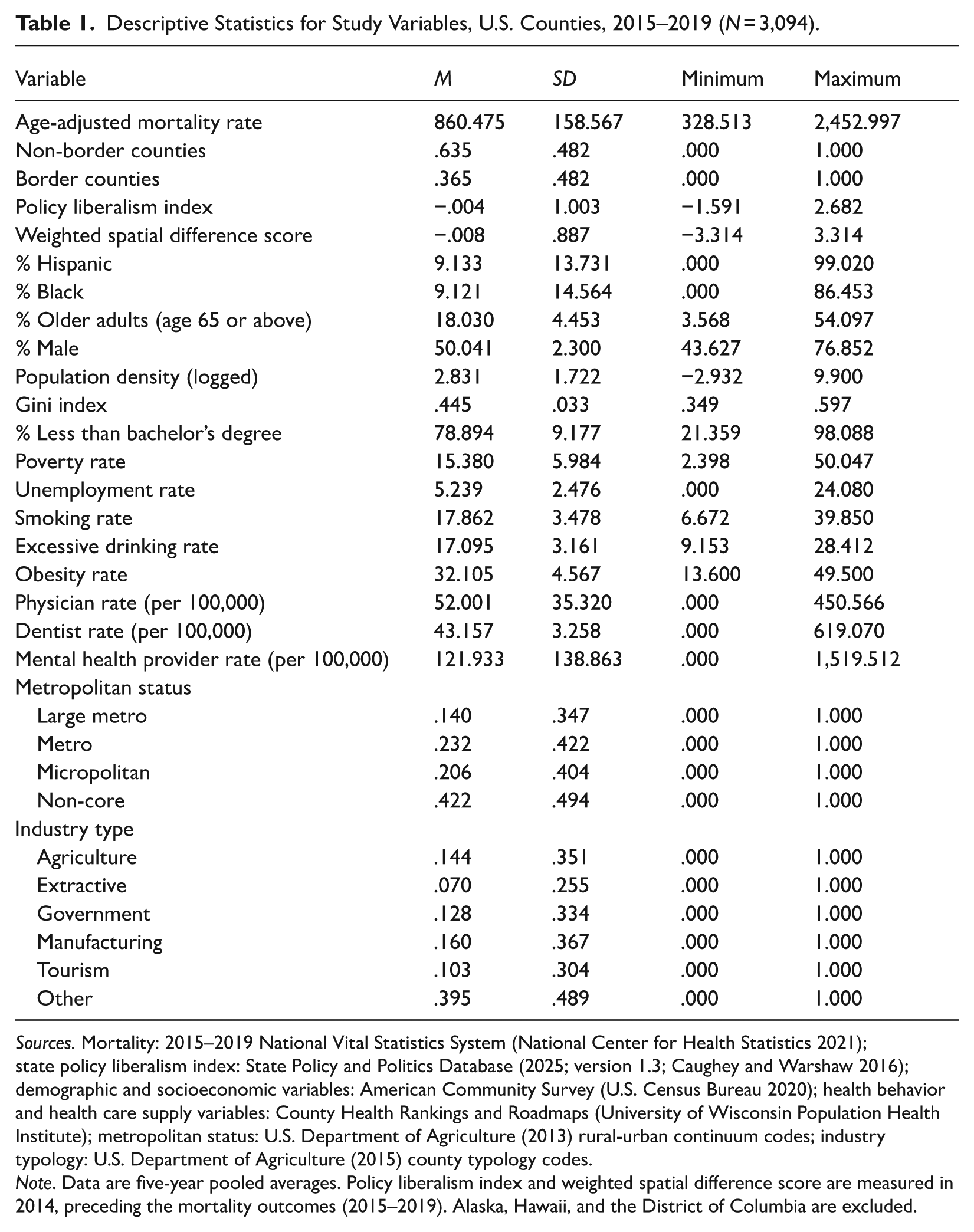
Sources. Mortality: 2015–2019 National Vital Statistics System (National Center for Health Statistics 2021); state policy liberalism index: State Policy and Politics Database (2025; version 1.3; Caughey and Warshaw 2016); demographic and socioeconomic variables: American Community Survey (U.S. Census Bureau 2020); health behavior and health care supply variables: County Health Rankings and Roadmaps (University of Wisconsin Population Health Institute); metropolitan status: U.S. Department of Agriculture (2013) rural-urban continuum codes; industry typology: U.S. Department of Agriculture (2015) county typology codes.
Note. Data are five-year pooled averages. Policy liberalism index and weighted spatial difference score are measured in 2014, preceding the mortality outcomes (2015–2019). Alaska, Hawaii, and the District of Columbia are excluded.
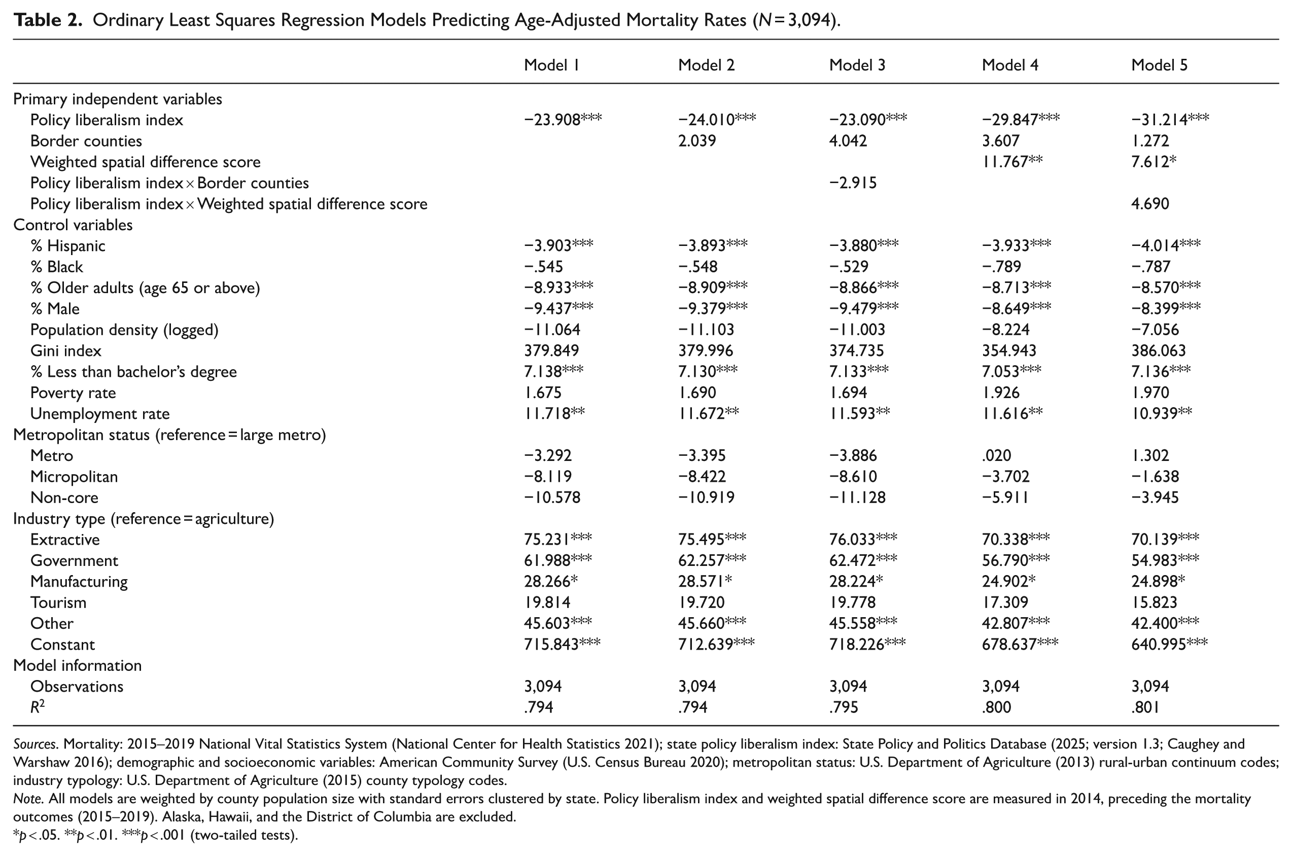
Table 2 presents results from five OLS regression models examining associations between state policy liberalism and county-level age-adjusted mortality rates, with all models employing population-weighted analysis and standard errors clustered at the state level to account for within-state correlation.
Ordinary Least Squares Regression Models Predicting Age-Adjusted Mortality Rates (N = 3,094).
Sources. Mortality: 2015–2019 National Vital Statistics System (National Center for Health Statistics 2021); state policy liberalism index: State Policy and Politics Database (2025; version 1.3; Caughey and Warshaw 2016); demographic and socioeconomic variables: American Community Survey (U.S. Census Bureau 2020); metropolitan status: U.S. Department of Agriculture (2013) rural-urban continuum codes; industry typology: U.S. Department of Agriculture (2015) county typology codes.
Note. All models are weighted by county population size with standard errors clustered by state. Policy liberalism index and weighted spatial difference score are measured in 2014, preceding the mortality outcomes (2015–2019). Alaska, Hawaii, and the District of Columbia are excluded.
p < .05. **p < .01. ***p < .001 (two-tailed tests).
Model 1 establishes the baseline relationship, demonstrating strong support for Hypothesis 1. The policy liberalism index shows a significant negative association with mortality rates (β = –23.908, p < .001), indicating that a 1 SD increase in policy liberalism corresponds to approximately 24 fewer deaths per 100,000 population after adjusting for county-level demographic, socioeconomic, and health characteristics. This finding confirms that more liberal state policy environments, characterized by stronger labor protections, comprehensive health care access, stricter tobacco and firearm regulations, and generous social safety nets, are associated with substantially lower mortality rates.
Model 2 adds border county status as a binary indicator. The coefficient is nonsignificant (β = 2.039, n.s.), suggesting that proximity to state boundaries per se does not predict mortality differences. The policy liberalism coefficient remains virtually unchanged (β = –24.010, p < .001), indicating that the direct policy effect persists regardless of geographic location at state borders. Model 3 incorporates an interaction between policy liberalism and border status. The interaction term is nonsignificant (β = –2.915, n.s.). This specification, however, treats all border counties within a state uniformly regardless of neighboring states’ policy environments. It cannot distinguish between counties bordering more liberal versus more conservative states. The weighted spatial difference score in Model 4 addresses this limitation by explicitly quantifying the direction and magnitude of cross-state policy contrasts weighted by geographic proximity to borders.
Model 4 introduces the weighted spatial difference score, which captures both the magnitude of cross-state policy contrasts and counties’ geographic proximity to borders. This specification directly tests Hypothesis 2 regarding spatial spillover effects. The weighted spatial difference score shows a positive and highly significant coefficient (β = 11.767, p < .01), providing strong support for the spillover hypothesis. Counties with positive scores (those bordering more conservative states) exhibit higher mortality rates than predicted by their own policies, while counties with negative scores (those bordering more liberal states) show lower mortality rates. For example, a county whose state is more liberal than its neighboring state by 1 SD of policy contrast (weighted spatial difference score = +1 SD) would experience approximately 12 additional deaths per 100,000 beyond what its own policy environment would predict (see Figure 2).
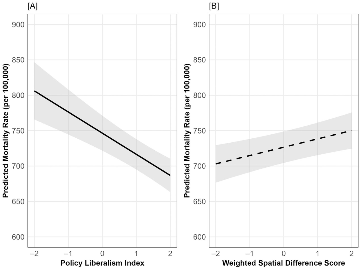
Association between primary independent variables and predicted age-adjusted mortality rate (per 100,000). (a) Policy liberalism index. (b) Weighted spatial difference score.
Importantly, accounting for spatial spillovers substantially increases the estimated direct policy effect. The policy liberalism coefficient rises to −29.847 (p < .001), a 24.8% increase from the baseline Model 1 estimate (–23.908). To formally assess whether this difference represents statistical bias rather than sampling variation, a cluster bootstrap test was conducted to compare coefficients across models (see Appendix Table 5, available in the online version of the article). The test confirms that the difference is statistically significant, demonstrating that models failing to account for spatial spillovers substantially underestimate the true direct effects of state policies on mortality. This underestimation occurs because conventional models implicitly attribute some spillover-driven mortality variation to measurement error or unexplained variance rather than recognizing it as a distinct spatial process.
Model 5 extends the analysis by testing whether spillover effects vary conditional on a county’s own policy environment, incorporating an interaction between policy liberalism and the weighted spatial difference score. The interaction term is positive but statistically nonsignificant (β = 4.690, n.s.), suggesting that spillover effects operate with similar magnitude across the policy liberalism spectrum. Counties in both liberal and conservative states appear equally susceptible to their neighbors’ policy environments. The main effects remain robust: policy liberalism (β = –31.214, p < .001) and spatial difference score (β = 7.612, p < .05). This pattern indicates that cross-border policy exposure influences mortality outcomes uniformly regardless of whether the focal county resides in a liberal or conservative state.
Table 3 presents the full mediation results for both hypothesized pathways. For health behavior diffusion (Hypothesis 3a), path b coefficients confirm that smoking (β = 12.200, p < .001) and obesity (β = 4.620, p < .001) are each significantly associated with higher county mortality, and excessive drinking shows a statistically significant association (β = −3.610, p < .05). However, path a coefficients reveal that the weighted spatial difference score shows no significant association with any health behavior mediator: smoking (β = .001, n.s.), excessive drinking (β = −.038, n.s.), or obesity (β = .110, n.s.). Consequently, all three indirect effects (ab) are nonsignificant, with bootstrap CIs spanning zero: smoking (β = .273, n.s., 95% CI [−2.39, 3.78]), excessive drinking (β = .278, n.s., 95% CI [−1.92, 3.27]), and obesity (β = .487, n.s., 95% CI [−.90, 2.67]).
Models Testing Spillover Mechanisms: Health Behaviors and Health Care Supply.
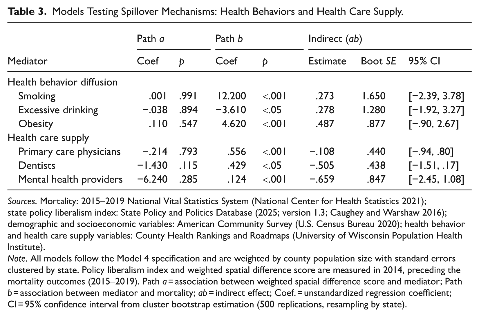
Sources. Mortality: 2015–2019 National Vital Statistics System (National Center for Health Statistics 2021); state policy liberalism index: State Policy and Politics Database (2025; version 1.3; Caughey and Warshaw 2016); demographic and socioeconomic variables: American Community Survey (U.S. Census Bureau 2020); health behavior and health care supply variables: County Health Rankings and Roadmaps (University of Wisconsin Population Health Institute).
Note. All models follow the Model 4 specification and are weighted by county population size with standard errors clustered by state. Policy liberalism index and weighted spatial difference score are measured in 2014, preceding the mortality outcomes (2015–2019). Path a = association between weighted spatial difference score and mediator; Path b = association between mediator and mortality; ab = indirect effect; Coef. = unstandardized regression coefficient; CI = 95% confidence interval from cluster bootstrap estimation (500 replications, resampling by state).
For health care supply spillovers (Hypothes 3b), path b coefficients confirm that physician availability (β = .556, p < .001), dentist availability (β = .429, p < .05), and mental health provider availability (β = .124, p < .001) are each significantly associated with mortality. Path a coefficients, however, show no significant association between the weighted spatial difference score and any health care supply mediator: physicians (β = −.214, n.s.), dentists (β = −1.430, n.s.), or mental health providers (β = −6.240, n.s.). All three indirect effects (ab) are nonsignificant: physicians (β = −.108, n.s., 95% CI [−. 94, .80]), dentists (β = −.505, n.s., 95% CI [−1.51, .17]), and mental health providers (β = −.659, n.s., 95% CI [−2.45, 1.08]). These results indicate that the first link in the mediation chain is absent.
Discussion
This study examined spatial spillover effects of state policy environments on county-level mortality rates, revealing three key findings that advance understanding of how policies shape population health across geographic boundaries. First, consistent with prior research, more liberal state policies are associated with significantly lower mortality rates, with a 1 SD increase in policy liberalism corresponding to approximately 24 fewer deaths per 100,000 population depending on model specification (Montez et al. 2022; Sun 2025). Second, and most importantly, the weighted spatial difference score reveals substantial cross-border spillover effects: Counties bordering states with more liberal policies experience lower mortality rates than their own policies would predict, while counties bordering more conservative states experience higher mortality rates. For example, a Texas county directly bordering New Mexico would experience approximately 23 fewer deaths per 100,000 compared to an interior Texas county, while a Texas county bordering Oklahoma would experience virtually no spillover effect. These examples demonstrate how spillovers operate bidirectionally, with effect sizes proportional to policy contrasts between neighboring states.
The mechanism analysis tests whether health behavior diffusion (Hypothesis 3a) and health care supply spillovers (Hypothesis 3b) explain the observed association between cross-border policy contrasts and county-level mortality. Neither pathway yielded statistically significant indirect effects. These null findings suggest that the two mechanisms (i.e., diffusion of health behaviors and cross-border access to health care infrastructure) do not account for the observed mortality spillovers. The mechanisms through which cross-state policy contrasts influence mortality likely operate through other pathways not examined here, including cross-border employment opportunities and wage spillovers, environmental regulations, housing affordability, transportation infrastructure, or other policy-relevant domains embedded in the comprehensive state policy liberalism index. As state policies influence mortality through multiple interconnected pathways (Hummer and Hamilton 2019; McFarland et al. 2023; Montez et al. 2022), disentangling these mechanisms requires individual-level data and more granular measurement of cross-border exposure than county-level estimates permit.
The weighted spatial difference score offers methodological advantages over conventional spatial approaches. Unlike standard spatial weights matrices that rely solely on geographic proximity, this measure quantifies relative policy contrasts while incorporating distance-based decay, directly operationalizing the theoretical mechanism as a substantive predictor. This approach addresses the limitations identified earlier: (1) Without relying on spatial regression models, it can simply measure policy contrast as a direct predictor, producing transparent coefficients showing how specific policy contrasts drive spillovers rather than averaging effects across neighbors into spatial autocorrelation parameters; (2) it incorporates distance decay into policy contrast measurement, recognizing that cross-border spillover potential varies with geographic proximity to state borders; and (3) it accommodates continuous, multidimensional policy indices rather than binary treatments, reflecting how policy environments consist of bundled regulations varying in degree along the liberal–conservative spectrum. By treating policy-based spatial exposure as a direct predictor in OLS regression, the measure enables straightforward interpretation showing that a 1-unit increase in the weighted spatial difference score is associated with 11.8 additional deaths per 100,000.
Accounting for spatial spillovers has important implications for policy evaluation. Models omitting the weighted spatial difference score underestimate direct policy effects by 24.8%, as confirmed by the coefficient difference test. This underestimation occurs because conventional models cannot distinguish mortality effects from a state’s own policies versus effects from neighboring states’ policies. Without accounting for cross-border exposure, these models incorrectly attribute spillover effects to unexplained variation, thereby underestimating direct policy effects (Harding et al. 2012; Horwitz and Polsky 2015). States with liberal policies appear to generate positive externalities for neighboring counties, while conservative policy environments impose harmful externalities across borders. Consequently, researchers examining state policy impacts without accounting for geographic context systematically undervalue policy interventions’ true effects. This has practical consequences for cost-benefit analyses, policy advocacy, and evidence-based policymaking as the health returns to policy investments exceed previously documented estimates.
Several limitations should be noted. First, the analysis cannot identify the specific mechanisms underlying spatial spillovers. Neither health behavior diffusion nor health care supply spillovers showed significant associations with cross-state policy contrasts, suggesting that other pathways, such as employment protections, housing affordability, or environmental regulations, may be operative. Future research should employ individual-level data to investigate these alternatives. Second, longitudinal analysis is needed to examine how spillover effects evolve as policy environments change since behavioral adaptations to shifting policy contexts may unfold gradually. Third, selection bias remains a concern as residents may strategically locate near border counties to access cross-state economic opportunities or social services, meaning border populations may differ systematically from interior populations in ways that independently affect health. Fourth, counties vary substantially in geographic area, particularly in the West, meaning many residents classified as living in border counties may practically live far from state boundaries. Finally, the health behavior mechanism analysis relies on CDC-modeled BRFSS estimates rather than direct measurements, so null findings for behavioral diffusion pathways should be interpreted cautiously.
Despite these limitations, the present study contributes to existing literature on liberal policy regimes and public health by demonstrating that policy effects extend beyond state boundaries through spatial spillover. In an era of increasing state policy polarization, findings of this study emphasize that efforts to improve population health through state policies should consider both direct effects and spatial dynamics.
Supplemental Material
sj-docx-1-hsb-10.1177_00221465261457832 – Supplemental material for Permeable Boundaries: How Neighboring States’ Policy Environments Shape Local Mortality Rates in the United States
Supplemental material, sj-docx-1-hsb-10.1177_00221465261457832 for Permeable Boundaries: How Neighboring States’ Policy Environments Shape Local Mortality Rates in the United States by Heeyoung Lee in Journal of Health and Social Behavior
Footnotes

Funding
The author received no financial support for the research, authorship, and/or publication of this article.
Declaration of Conflicting Interests
The author declared no potential conflicts of interest with respect to the research, authorship, and/or publication of this article.
Supplemental Material
Supplemental material is available online.
Author Biography
References
Supplementary Material
Please find the following supplemental material available below.
For Open Access articles published under a Creative Commons License, all supplemental material carries the same license as the article it is associated with.
For non-Open Access articles published, all supplemental material carries a non-exclusive license, and permission requests for re-use of supplemental material or any part of supplemental material shall be sent directly to the copyright owner as specified in the copyright notice associated with the article.
