p -Values as QWERTY: Curating Evidence in the Computational Era

Abstract

McShane et al.'s (2024) wide-ranging critique of null hypothesis significance testing provides a number of specific suggestions for improved practice in empirical research. This commentary amplifies several of these from the perspective of computational statistics—particularly nonparametrics, resampling/bootstrapping, and Bayesian methods—applied to common research problems. Throughout, the author emphasizes estimation (as opposed to testing) and uncertainty quantification through a comprehensive process of “curating” a variety of graphical and tabular evidence. Specifically, researchers should be encouraged to estimate the quantities that matter, with as few assumptions as possible, in multiple ways, then try to visualize it all, documenting their pathway from data to results for others to follow.

Keywords

null hypothesis significance testing computational statistics nonparametrics bootstrapping

Background

Many of you are reading this, just as I composed it, on a device equipped with a QWERTY-style keyboard. Devised in the 1870s to split common English digrams across the hands to avoid jamming the internal mechanisms of the day, it has since achieved near-universal prevalence among Latin-alphabet keyboard layouts, decades after a technological transition away from the mechanical typewriters that gave rise to them. This seemingly anomalous inefficiency does not lack for scholarly attention (e.g., David 1985; Hossain and Morgan 2009), but the boiled-down version suggests an amalgam of human factors (e.g., retraining), supply-side production efficiencies, and various user-borne costs (e.g., the need to support multiple keyboard styles, additional input errors). So potent are these combined effects that one can envision the first humans traveling to Mars and beyond pecking out their Earth-bound messages via QWERTY.

The extended metaphor underlying this commentary is that null hypothesis significance testing’s (NHST's) summarization of all evidence via dichotomized p-values¹ (i.e., “statistical [non]significance”) are QWERTY's statistical doppelgangers: historical “frozen accidents” encased in amber so durable that only collective concerted effort can dislodge them. The metaphor is surprisingly literal and translatable: “statistical significance” is a cultural relic of a time when computation was costly, printed journal space was “precious,” online storage wasn’t a thing, p-values needed to be tediously extracted from tables indexed by degrees of freedom,² models were typically ordinary least squares, and anything beyond z, t, χ², and F was exotic and thereby suspect. Scholarly journals tended to enforce this hegemony, requiring that hypotheses be explicitly stated, in NHST form (that is, asserting the opposite of what one hoped to show), and receive formal nonsupport via p-values crossing the α = .05 Rubicon into the hallowed ground of “statistical significance.” That is, exactly the sort of one-size-fits-all dichotomization procedure that many statisticians have inveighed against for nearly a century (e.g., Fisher 1926; Pearson 1935). We no longer live in a time when the forces giving rise to NHST and p < .05 exist, yet, just like QWERTY, they show few signs of loosening their talons.

While none of the many points raised in McShane et al. (2024) are off the mark, a few bear especial emphasis and exemplification. One seems particularly critical: p-values, correctly interpreted as compatibility, should not be tossed aside as conceptually misguided. Just like salt was once scarce and therefore valuable, its present abundance doesn’t render it worthless. That is—and as the title of this commentary suggests—living in an era of computational abundance doesn’t suggest that easy-to-calculate data summaries should be supplanted entirely by complex graphical, tabular, or other illustrations. There are advantages to procedural standardization and community guidelines, and including p-values as part of a more comprehensive curation of evidence is entirely sensible.

The remainder of this article concerns what, exactly, practicing researchers—who are not statisticians and are concerned with communicating their salient findings—might consider. For convenience, it can summarized as a six-step procedure with deliberately alliterative endings: curation, distillation, illustration, integration, and interpretation, abundantly supplemented by documentation. In very broad terms, these consist of the following:

Curation: providing as much “raw material” as institutional review boards and nondisclosure agreements allow, ideally everything to enable other researchers to explore the original data (or close proxies) in fresh ways.

Distillation: a process of directed funneling that starts with the original data and examines it at successively greater degrees of aggregation and summarization.

Illustration: using graphical tools, online appendices, online archives (e.g., OSF), and creativity to bring both theoretically important and empirically remarkable aspects of the data to the fore.

Integration: summarizing quantities that those consuming the research care about, such as strength of evidence, robustness to alternative assumptions and methods, effects sizes, confidence intervals, and—whenever possible—translations into observable, meaningful metrics.

Interpretation: offering some sense of which quantities or findings seem well-estimated, substantial, and/or important.

Documentation: providing all critical details needed to follow and recreate the analyses, including intermediate estimation results, packages, code, preparation steps, and so on. This includes, importantly, studies and analyses that did not appear in the final manuscript.

The purpose of these procedures is, loosely speaking, the idealized version of Doing Science. Richard Feynman, in something of a dig at the profession, went so far as to view scientific research as the opposite of advertising: “The idea is to try to give all of the information to help others to judge the value of your contribution; not just the information that leads to judgment in one particular direction or another. The easiest way to explain this is to contrast it with advertising” (Feynman 1995, p. 57). Composer Igor Stravinsky, when asked how he conceived his most iconic work, famously responded, “I am the vessel through which Le Sacre passed” (Stravinsky and Craft 1962, pp. 147–48). We, too, should be vessels through which our work passes from ideation through realization, neutral ciphers to convey with equal emphasis what is supported and what is not. To take the Bayesian perspective (more on this later), we start with a prior (what we knew before our data rolled in) and then condition on that data to obtain our posterior (what we know afterward), warts and all. This will require a commitment from journal editors and reviewers that radical transparency is valorized, a field-wide transition from “advertising” our work to trenchantly, doggedly documenting all it tells.

Descending from the pulpit to the trenches: How can practicing researchers accomplish this, without turning into data scientists or archivists? One answer, which is less snarky than it would first appear, is to avail of the fact that marketing is a hybrid discipline teeming with “quants”—empirical and applied statisticians in particular—eager to collaborate, because we are interested in the same substantive issues as everyone else. But, to paraphrase Geoff Hinton when asked how he learned so much statistics, “I realized it was altogether more pleasant to become a statistician than to befriend one.” For those who view the trade-off through a similar lens, below are some suggestions in line with the main theme of this commentary: computation is cheap, so use it.

As an umbrella—albeit one that may not appear particularly protective—we should all become more familiar with three classes of techniques: nonparametrics, resampling/bootstrapping, and Bayesian modeling. “Familiar” does not mean “expert,” no more than users of PROC GLM have delved into its algorithms. Next, I provide some examples of how to use such methods in transparent ways, but, to clarify why it's worth the effort, as McShane et al. (2024) also emphasize, good statistical practice should strive above all to achieve two goals:

Estimate the Thing That Matters. “Science” is largely concerned (some might say obsessed) with quantification. In marketing, this might entail the effect of increased promotion frequency, colored type in a print ad, or making a product more sustainable. Regardless, there are always a set of “estimands” we seek to extract, and such point estimates should, following McShane et al. (2024), not only be the ones “most compatible” with the data but also be as free as possible from restrictive assumptions that were imposed historically due to lack of computational power, including (but hardly limited to) functional form (e.g., linearity), balanced cell sizes, homoskedasticity, sample selection, uncorrelated errors, nonrandom missingness, endogeneity … the list goes on. When the dust settles, statements like “a wide range of models that relax [insert unverified assumptions] provide estimates that vary no more than 7% from PROC ANOVA” not only help quantify key estimands but provide evidence that the statistical model itself is not strongly influencing downstream substantive conclusions based on it.

Show How Well You Estimated It. Placing standard errors in parentheses next to estimates is ubiquitous, a wholly sensible practice when space and computation were scarce. There is a deep literature on “uncertainty quantification” and propagation, and the excellent Wikipedia article lists (at the time of writing) seven sources of uncertainty and two distinct theoretical types.³ Needless to say, these cannot all be encompassed in a single quantity like the standard error, which (also needless to say) is highly model-dependent. McShane et al. (2024) make some prudent graphical suggestions to alleviate some of these concerns, which are supplemented here.

The point of all this is to initiate a paradigm shift from testing (NHST and its dichotomized p-values) to estimation. Or, more tellingly, from assuring a reader that some quantity is not actually zero—what McShane et al. (2024) remind us is, in marketing, essentially always false—to providing comprehensive evidence regarding its actual size and importance, taking various forms of “known unknowns” (Rumsfeld 2011) into account.

An Example, Revisited

McShane et al. (2024) provide an extended example to serve as a (deliberately) “painfully complete” explication of experimental results. It involves a common binomial sampling problem, where ${\hat{p}}_{1} = .55 and {\hat{p}}_{2} = .45$ . The usual “frequentist” analysis—which often relies on unchecked assumptions of asymptotic normality—goes off the well-loved formulas,⁴

z = \frac{{\hat{p}}_{1} - {\hat{p}}_{2}}{\sqrt{\bar{p} (1 - \bar{p}) (\frac{1}{n_{1}} + \frac{1}{n_{2}})}}, \bar{p} = \frac{n_{1} {\hat{p}}_{1} + n_{2} {\hat{p}}_{2}}{n_{1} + n_{2}},

which in this case suggested (given the rest of their example, and assuming cell balance) that n₁ and n₂ were both around 400. Such samples sizes are more than enough for the usual tests to be valid, but … what if we weren’t sure, or had a contingency table some of whose cells were far sparser? Given that we are, indeed, in the computational era and computers never sleep, why not just sample for what we want, instead of shoehorning everything into a z-statistic?

One might think this is a lot to ask, and requires knowing how to set up such simulations. However, to illustrate horrific research practice but the very best of intentions, I have pretended (sadly, only mildly) to know little about the statistical programming language R, and turned to a large language model (ChatGPT 4.0) to help me. And, to illustrate the use of archiving, all resulting annotated code is included in the Web Appendix. Just to keep things simple, here is the workflow:

Steps in Simulating Useful Quantities for the Two-Sample Binary Data Example

Start off with your data, which consists of two binary samples of size 400, the first with 55% ones, the second with 45% ones (here, I generate it for illustration).

Calculate whatever you’re after by sampling again and again, then graphing the results.

It's part 1 that requires some additional specifics, but the general tenor should be clear enough. We can start by doing exactly the analysis we want to veer away from: simulating the usual p-value based on NHST. To do so requires taking the two samples, lumping them together (because the null hypothesis says they’re from the same population), splitting them randomly again and again into two new samples of the same sizes, then seeing how often they differ by more than the original samples did. Child's play for ChatGPT, which also helps generate a histogram and overlay a kernel density estimate, as in Figure 1.

Figure 1.

Histogram with Kernel Density of Differences in Proportions.

The key is that we can simply count how often the result (here, based on 100,000 draws) is more than 10% in either direction, and that turns out to be 505/100,000 or .00505. As expected, this compares fairly well with the theoretical one of z = 2.828 and p = .00466, but not perfectly, because the actual tails, which represent relatively rare events (<.5% of the time), appear to be a bit thicker than the asymptotic distribution would suggest, and because we have still used our actual data, not taken new samples from some theoretically infinite population.

Many readers will wonder why one would carry out such an exercise when classical tools and tests work quite well. Suppose that the manuscript containing this analysis received the following thoughtful critique from Reviewer 2: “The ratio in the first versus the second condition is 1.222, which the seminal article of Reviewer 2 suggests should be at most 1.1,” while Reviewer 3 brings up “work from psychophysics suggesting that p₂/(p₁)^3/2 should be roughly 1 (which would also hold under equal proportions), not the 1.10 value observed in your data.” They both posit looking at particular values of specific quantities computed from the data, and try as you might no standard tests of such hypotheses are to be found. How can one “estimate the thing that matters” and “show how well you estimated it”?

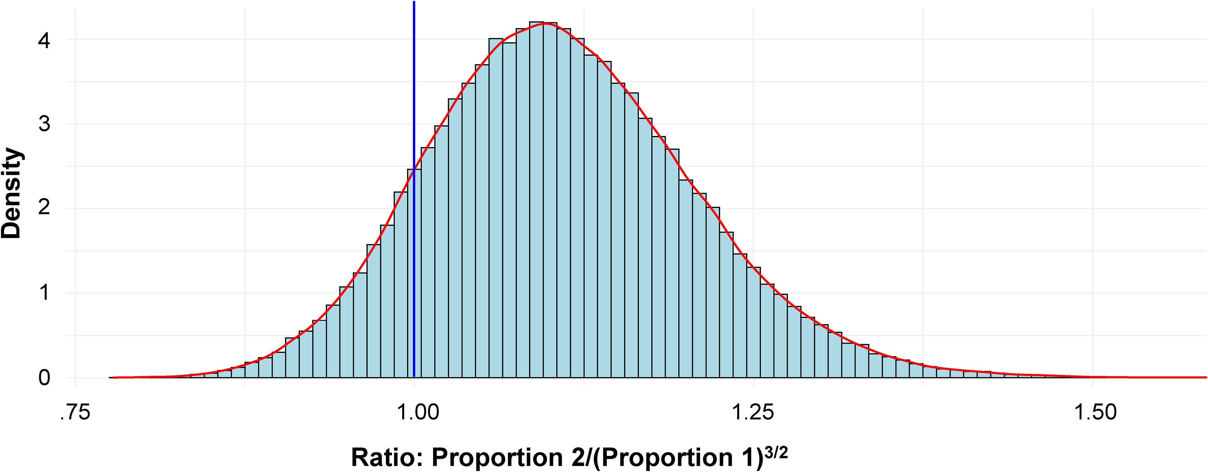
The answer is to jettison the NHST perspective, which posits mind-twisting counterfactuals like “suppose we drew samples just like these two a bajillion times from the same population, and we want to know how often something as or more extreme …,” even though we did no such thing. Instead, we can take the “Bayesian” perspective: the data are the data, so what else can we say based on them? One can answer essentially any question about the “proportions” above by simply bootstrapping, a procedure that will be familiar to researchers in consumer behavior who’ve done a mediation analysis (that is, everyone), since the key test in that analysis multiplies two other (asymptotically normal) distributions together, yielding a Frankendensity with no “named” form, even in large samples.⁵ In our case, let's carry out the analogous procedure: sample (with replacement) from both data sets, and simply compute anything we’d like. ChatGPT wrote this R code rapidly and, with just a little aesthetic tweaking, provided the following to address all our questions—that is, the distributions of: the difference in proportions, the ratio of proportions, and Reviewer 3's quantity of interest, p₂/(p₁)^3/2, as depicted in Figure 2.

Figure 2.

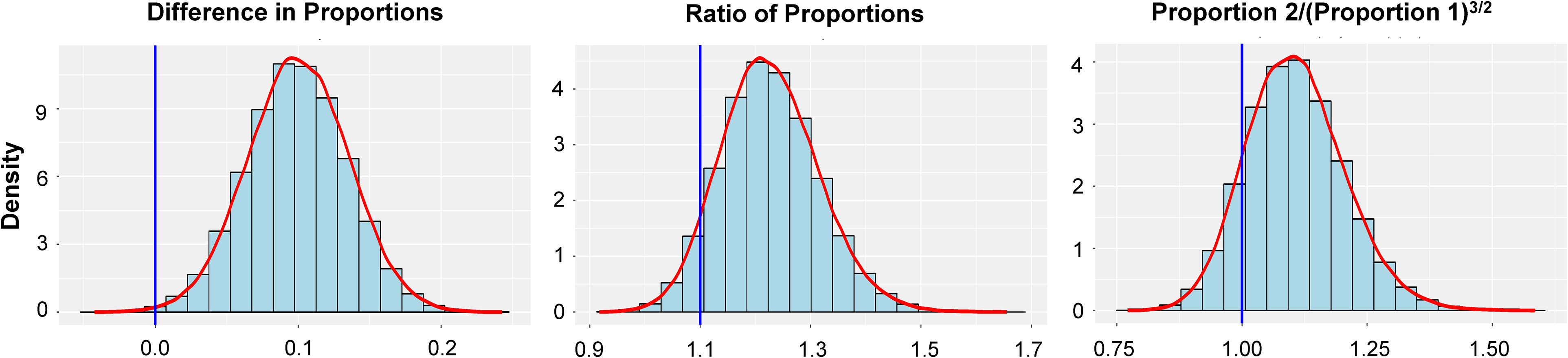
Histograms of Three Quantities Computed by Bootstrapping.

In each case, we have superimposed a vertical line for a quantity we’re interested in, but the important point is that we have provided a full account of The Thing We Want to Estimate and have not made any assumptions about the data-generating process, the eventual shape of the distribution, or even what we’re actually hoping to test! That is, no null hypothesis in sight. We can also easily approximate, respectively, the proportion of the 100,000 replications below 0 (.00222), 1.1 (.06837), and 1 (.13164).⁶ The first of these quantities checks well against the two-sided p = .00466 from our classical analysis. But the other two have no classical counterpart, yet we can respond to Reviewer 2 that the data are indeed reasonably compatible with the true value being 1.1 and something similar to Reviewer 3 (hopefully not tanking our manuscript's chances, something editors can help with by evaluating research less on rejecting null hypotheses, and more on fully examining what the data suggest).

But isn’t this burdensome? Not really: it all took under 40 minutes from the first ChatGPT query, including all resampling and graphics generation, and I’m not particularly adept at prompt engineering.⁷ Moreover, it allows us to engage in curation (“here are all the data”), distillation (“let us examine it in several different ways”), illustration (“here are the distributions”), integration (“generalizing across analyses …”), interpretation (“… we see that only some of our hypotheses are strongly compatible with the data”), and documentation (“all the code for analysis and graphical illustration, as well as intermediate output itself, is available at …”). Ideally, one could carry this out for different models, methods, degrees of granularity, and so on, and store it in “notebook” fashion for editors and eventual readers to dynamically interact with.⁸

Decontaminating Results from Assumptions: Practical Nonparametrics

In the dark time before the computational era, many assumptions were invoked because not doing so strained the resources of the day. As McShane et al. (2024) remind us that the null (“no effect”) is never true, they also remind us that the same can be said of all our background assumptions. Among the most pernicious is linearity—nature abhors a line as much as a vacuum⁹—which can be viewed in economic terms as a constant marginal effect or statistically as a strong regularization on curvature (none), among other lenses. We single out linearity for its special and often unacknowledged place in empirical analysis, and so are especially fortunate nowadays that there are simple ways to leverage well-vetted, powerful, and automatized techniques to, if not banish linearity entirely, view it as a testable special case of something less “assumptive.”

But, more broadly, nonparametric methods automatically adapt to the size and complexity of the data, without tedious post hoc decisions based on researcher-chosen metrics such as Akaike or Bayesian information criteria. Among the most powerful and easiest to apply are in the generalized additive models (GAM; Hastie and Tibshirani 1990) category, which, despite decades in the statistical literature, superb software support (MGCV in R, GAM in STATA, PyGAM in Python), and tens of thousands of citations, have appeared only roughly a dozen times in premier marketing journals (and just once in the history of Journal of Consumer Research and Journal of Consumer Psychology combined). For example, let’s use some real data—that, in line with our philosophy, are archived with this article, along with all code and output—from an ongoing project. The specific context isn’t important, but suggests that some quality measured by natural language processing (NLP) is consistently positively related to respondents' likelihood of picking the right answer (a binary variable). But it's hard to imagine a theory suggesting the relationship between an NLP measure and a latent utility is linear. How can we account for this and also quantify (a limited, but typical, form of) uncertainty? It's as simple as, alongside the linear model y ∼ x, also running a nonlinear one, y ∼ s(X), that automatically matches the complexity of the data. The graphical results appear in Figure 3.

Figure 3.

GLM Versus GAM Predictions, with Error Quantification.

We can see—literally—that for all smaller values of the NLP measure, the flexible model seems relatively compatible with the linear predictor, but for its highest values, it is far less so. Moreover, it seems that the linear fit may be overly influenced by the data for smaller values, leading to potentially erroneous predictions at the upper end, where there is far less data.¹⁰ None of this required NHST or p-values, and, in fact, one can ask essentially any question about either model by simply bootstrapping the data; for example, whether the GAM is compatible with a monotonic function (answer: yes) or a flat function (answer: no) or more exotic questions like whether the upper half of the data have a slope at least 50% more than the lower half (I didn’t try … but, because the data are archived, you can!)

Baron and Kenny: We Hardly Knew Ye

All of this can be put to immediate use by behavioral researchers who do mediation analysis, extending the ideas in the landmark article by Baron and Kenny (1986). This idea is hardly new, and in fact there is an entire chapter by Imai et al. (2010) and the associated mediate R package that automatically accommodates nonlinear (nonparametric) modeling, bootstrapping for focal quantities, and full uncertainty quantification. Subsequently, I discuss an even more capable software solution written by marketing academics for similar purposes.

Be Bayesian, At Least Sometimes

In their deservedly celebrated article, Simmons, Nelson, and Simonsohn (2011) call out another downside of the tyranny of NHST—namely, p-hacking—and also share practical advice for avoiding it. Among their “nonsolutions” was the Bayesian approach, which, it must be admitted, can indeed inject additional “researcher degrees of freedom.” Viewed through a wider lens, however, Bayesian methods allow researchers the right kind of leeway: to posit models that flexibly capture the interactions of many quantities of interest, to regularize them appropriately (e.g., hierarchical models), and to fully account for their mutual uncertainty. As laid out in the treatise by Betancourt (2018), Bayesian analyses help focus on specific quantities of interest by marginalizing out (i.e., doing high-dimensional integration over) everything else. Bayesian estimation used to have, to put it euphemistically, a steep learning curve, but all that changed with general-purpose modeling environments like Stan (Carpenter et al. 2017) and prepackaged analyses built into major software packages like STATA, SAS, and SPSS.

But to press both the point and my luck, I simply asked ChatGPT to generate a Stan program, run entirely from R, that would produce a posterior distribution for Reviewer 3's quantity of choice, p₂/(p₁)^3/2, conditional on the original data. This it did immediately, and, because I was just interested in one focal estimand, it ran in under 5 seconds for ten chains of 10,000 draws (i.e., 100,000 total), providing this useful distributional summary (n_eff and Rhat are ways to assess parameter estimation adequacy, and both are terrific here). See Figure 4 and the accompanying table:

10 chains, each with iter = 20,000; warmup = 10,000; thin = 1; postwarmup draws per chain = 10,000, total postwarmup draws = 1e + 05.
	Mean	2.50%	25%	50%	75%	97.50%	n_eff	Rhat
p1	.55	.501	.533	.55	.567	.598	90,603	1.000
p2	.45	.402	.433	.45	.467	.499	93,519	1.000
ratio	1.109	.932	1.041	1.104	1.171	1.314	90,850	1.000

Figure 4.

Posterior Distribution of Proportion 2/(Proportion 1)^3/2.

We can also hope to satisfy Reviewer 3 by calculating what proportion of the graph lies below 1, yielding .12656, a bit less than the earlier simulation result of .13164, which perhaps reflects the nature of the prior distribution (something we can assess computationally by simply trying out other priors).¹¹

W(h)ither Machine Learning?

One might ask why we need “models” at all, when machine learning presents its bewitching black boxes. There is no questioning—especially in an article that illustrates the ease of doing computational statistics with the help of ChatGPT—the power and versatility of machine learning techniques. They can be viewed, however, as simply another sort of nonparametric model, with the advantage and the curse of including arbitrarily high interactions of nonlinear terms and automatically pruning back, through specialized regularization techniques, those that don’t generalize out of sample. I can only refer the reader to the extensive critique of Rudin (2019), whose article has one of the least enigmatic titles in recent memory: “Stop Explaining Black Box Machine Learning Models for High Stakes Decisions and Use Interpretable Models Instead.” An advantage of model-building is that one knows what one has built and can examine (posterior distributions of) quantities arising from the model as a kind of sniff test. By contrast, it's unclear how to even accommodate uncertainty in machine learning models (Abdar et al. 2021; Gal and Ghahramani 2016); empirical researchers using them are faced with a trade-off between fidelity and explicability and need to carefully think through which takes pride of place in their work.

Importance of Heterogeneity

The number of studies in empirical marketing incorporating heterogeneity is vast, as are the methods for doing so, which include discrete and continuous mixtures as well as nonparametric methods. It's been overwhelmingly demonstrated that heterogeneity is substantively important and yields far more accurate predictions when accommodated in statistical models. But Hutchinson, Kamakura, and Lynch (2000) took this one step further by showing that well-verified behavioral effects (e.g., preference reversals) could also be “explained” by a failure to accommodate heterogeneity. That is, what appeared to be substantive and vetted may have been a mirage because researchers were adopting computationally cheaper modeling approaches. Nowadays, there are many out-of-the-box tools for incorporating heterogeneity, awaiting their widespread application in behavioral marketing and beyond.

Importance of Meaningful Metrics

Even when heterogeneity is accommodated, it is often by imposing a normal distribution for parameters in some latent construct like “consumer utility.” This was largely—to keep with the theme—because early computational methods made use of “conjugacy” to enable efficient calculation. Yet Sonnier, Ainslie, and Otter (2007) showed that specifying heterogeneity in some “interpretable” or “observable” quantity like willingness to pay often yielded different substantive answers than doing so for utility itself, using the same data. That is, the cheaper computational method could bias substantive findings. But today we have general purpose software tools (like Stan) and powerful dedicated ones (like Helveston's [2022] logitr for this exact problem) that free the analyst from enacting such assumptions merely for computational convenience. This is in line with the shift in the Bayesian community from difficult-to-calculate and -convey measures like log marginal density to “posterior predictive checks”: data-informed metrics that make intuitive sense while fully accommodating uncertainty.

Importance of flexibility and illustration

If nonparametrics are good, and Bayesian is good, Bayesian nonparametrics must be super-good. And indeed they are, but the difficulty of application—which has now largely waned—was a longtime impediment. As an example of their power and elegance, one need look no further than Dew and Ansari (2018), who used Gaussian processes to not only push the state-of-the-art of customer base analysis but also to demonstrate how to (quite fetchingly) visualize cyclical, short-term, and long-term time trends reflecting complexity dictated by the data, with full error quantification. Their paper is an object lesson in applying models that used to be daunting computationally and using them to create actionable, visual “dashboards”—ones practicing managers can use—in something like real time.

Importance for consumer behavior researchers

Although this commentary is not differentially directed toward behavioral scholars, a good deal of it might generate well-intentioned eye-rolling from practicing researchers who “have enough to do already” without delving into computational methods. Anticipating this, Wedel and Dong (2020) built their BANOVA tool (along with dedicated case-usage studies) as a Bayesian Swiss Army Knife for repeated-measures experiments, providing effect sizes (“what we want to estimate”), Bayesian uncertainty quantification (“how well we’ve estimated it”) as well as planned comparisons, spotlight/floodlight, and complex combinations of mediation and moderation. That is, using computational tools to alleviate assumptions and extract meaning from real-world data.

All of this is the tip of the proverbial iceberg, but should help support a central contention: summarizing the evidence “against” a null hypothesis in a single (p) value was (perhaps) sensible at a time in history when computation and space were at a premium. Because that time is long past, researchers, referees, editors, and readers would do well to jointly transition to computationally accommodating a variety of analyses that provide a robust, graphically informed account of the substantive content of our data.

Conclusion

McShane et al. (2024) cover a great deal of ground that I’ve not touched on here. For example, they highlight a remarkable fact in their introduction: two studies can differ greatly in their “statistical (non)significance” from zero (p = .005 and p = .194, respectively) but not from one another (p = .289), in some conceptual quasi-violation of the triangle inequality. It's like saying, “I’m near you; my friend is far from you; yet my friend and I are standing right next to each other.” This seeming anomaly highlights that studies that “fail to differ from zero” can also fail to differ from much of anything, because they are underpowered, imprecise, or both. As McShane et al. show, graphical and computational tools can illuminate such scenarios in a way that tables of p-values simply can’t.

Hopefully several high-level takeaways have emerged here. One is most decidedly not “when in doubt, ask a large language model to generate your code.” Rather, this was done to demonstrate that, contrary to the situation a decade ago—when casually suggesting a Bayesian analysis was an act of cruelty—both canned and bespoke computational tools are abundant, powerful, and far easier to directly apply than ever before. But, more importantly, the all-encompassing paradigm of “propose that the thing you want is actually zero and hope that a single quantity falls below .05” not only is well past its sell-by date but encourages p-hacking and other practices that cloud the scientific record. Instead, it should be replaced by something like “estimate the thing(s) that matter, with as few assumptions as possible, in multiple ways, then try to visualize it all, documenting your pathway from data to results for others to follow.” There are variations on this theme, of course, but they are all superior to the “p < .05” one.

To paraphrase David Blei in a related context, such a transition will be “more a triumph of sociology than technology” (personal correspondence). Because research only makes an impact if it is published, the overseers of that process—editors and reviewers alike—should discourage tables of alluringly meager p-values in favor of full reporting and disclosure, including for studies and manipulations that did not pan out. Well-executed research that doesn’t uncover what theory or intuition suggests can be dispositive and, when integrated via eventual meta-analysis (again, using computational tools on provided data), offer nuanced retrospective insight that single studies cannot. In short, as a field we must transition from dichotomizers to curators. To that end, McShane et al. (2024) provide an implementable and sensible blueprint to get us all comoving in the right direction.

Footnotes

Acknowledgments

The author would like to thank Gwen Ahn, Eric Eisenstein, and Blake McShane for “comments on the Comment,” and use of their data for illustrative purposes.

Declaration of Conflicting Interests

The author(s) declared no potential conflicts of interest with respect to the research, authorship, and/or publication of this article.

Funding

The author(s) received no financial support for the research, authorship, and/or publication of this article.

ORCID iD

Fred Feinberg

Notes

References

Abdar

Moloud

Pourpanah

Farhad

Hussain

Sadiq

Rezazadegan

Dana

Liu

Ghavamzadeh

Mohammad

Fieguth

Paul

Cao

Xiaochun

Khosravi

Abbas

Acharya

U. Rajendra

Makarenkov

Vladimir

, and Saeid Nahavandi (2021), “A Review of Uncertainty Quantification in Deep Learning: Techniques, Applications and Challenges,” Information Fusion, 76, 243–97.

Baron

Reuben M.

Kenny

David A.

(1986), “The Moderator-Mediator Variable Distinction in Social Psychological Research: Conceptual, Strategic, and Statistical Considerations,” Journal of Personality and Social Psychology, 51 (6), 1173–82.

Betancourt

(2018), “A Conceptual Introduction to Hamiltonian Monte Carlo,” arXiv preprint, https://doi.org/10.48550/arXiv.1701.02434.

Carpenter

Bob

Gelman

Andrew

Hoffman

Matthew D.

Lee

Daniel

Goodrich

Ben

Betancourt

Michael

Brubaker

Marcus A.

Guo

Jiqiang

Peter

Riddell

Allen

(2017), “Stan: A Probabilistic Programming Language,” Journal of Statistical Software, 76 (1), 1–32.

David

Paul A.

(1985), “Clio and the Economics of QWERTY,” American Economic Review, 75 (2), 332–37.

Dew

Ryan

Ansari

Asim

(2018), “Bayesian Nonparametric Customer Base Analysis with Model-Based Visualizations,” Marketing Science, 37 (2), 216–35.

Feynman

Richard P.

(1998), “Cargo Cult Science,” in The Art and Science of Analog Circuit Design, Jim Williams, ed. Elsevier, 55–61.

Fisher

Ronald Aylmer

(1926), “The Arrangement of Field Experiments,” Journal of the Ministry of Agriculture, 33, 503–13.

Gal

Yarin

Ghahramani

Zoubin

(2016), “Dropout as a Bayesian Approximation: Representing Model Uncertainty in Deep Learning,” in International Conference on Machine Learning. PMLR, 1050–59.

10.

Hastie

Trevor J.

Tibshirani

Robert J.

(1990), Generalized Additive Models. Chapman and Hall.

11.

Helveston

John P.

(2022), “logitr: Fast Estimation of Multinomial and Mixed Logit Models with Preference Space and Willingness to Pay Space Utility Parameterizations,” arXiv preprint, https://doi.org/10.48550/arXiv.2210.10875.

12.

Hossain

Tanjim

Morgan

John

(2009), “The Quest for QWERTY,” American Economic Review, 99 (2), 435–40.

13.

Hutchinson

J. Wesley

Kamakura

Wagner A.

Lynch

John G.

Jr. (2000), “Unobserved Heterogeneity as an Alternative Explanation for ‘Reversal’ Effects in Behavioral Research,” Journal of Consumer Research, 27(3), 324–44.

14.

Imai

Kosuke

Keele

Luke

Tingley

Dustin

Yamamoto

Teppei

(2010), “Causal Mediation Analysis Using R,” in Advances in Social Science Research Using R, Hrishikesh D. Vinod, ed. Springer, 129–54.

15.

Mandelbrot

Benoit B.

(1982), The Fractal Geometry of Nature, Vol. 1. New York: WH Freeman.

16.

McShane

Blakeley B.

Bradlow

Eric T.

Lynch

John G.

Jr. Meyer

Robert J.

(2024), “'Statistical Significance' and Statisical Reporting: Moving Beyond Binary,” Journal of Marketing, 88 (3), 1–19.

17.

Pearson

Karl

(1935), “Letter to the Editor: Statistical Tests,” Nature, 136, 550.

18.

Rudin

Cynthia

(2019), “Stop Explaining Black Box Machine Learning Models for High Stakes Decisions and Use Interpretable Models Instead,” Nature Machine Intelligence, 1 (5), 206–15.

19.

Rumsfeld

Donald

(2011), Known and Unknown: A Memoir. Penguin.

20.

Shapiro

Bradley T.

Hitsch

Günter J.

Tuchman

Anna E.

(2021), “TV Advertising Effectiveness and Profitability: Generalizable Results from 288 Brands,” Econometrica, 89 (4), 1855–79.

21.

Simmons

Joseph P.

Nelson

Leif D.

Simonsohn

Uri

(2011), “False-Positive Psychology: Undisclosed Flexibility in Data Collection and Analysis Allows Presenting Anything as Significant,” Psychological Science, 22 (11), 1359–66.

22.

Sonnier

Garrett

Ainslie

Andrew

Otter

Thomas

(2007), “Heterogeneity Distributions of Willingness-to-Pay in Choice Models,” Quantitative Marketing and Economics, 5, 313–31.

23.

Stravinsky

Igor

Craft

Robert

(1962), Expositions and Developments. University of California Press.

24.

Wedel

Michel

Dong

Chen

(2020), “BANOVA: Bayesian Analysis of Experiments in Consumer Psychology,” Journal of Consumer Psychology, 30 (1), 3–23.

25.

Zhang

Jie