Early Cost Realization and College Choice

Abstract

Student loans defer the cost of college until after graduation, allowing many students access to higher lifetime earnings and colleges and universities they otherwise could not afford. Even with student loans, however, the authors find that students psychologically realize the financial costs of a college education long before their loan repayments begin. This early cost realization frames financial decisions between most pairs of colleges as an intertemporal trade-off. Students choose between investments with (1) smaller short-term costs but smaller long-term returns (a lower-cost, lower-return [LC-LR] college) and (2) larger short-term costs but larger long-term returns (a higher-cost, higher-return [HC-HR] college). The authors find that early cost realization increases preferences for LC-LR colleges—preferences that could reduce lifetime earnings—in both simulations and experiments. Preferences for LC-LR colleges are pronounced among financially impatient students and in choice pairs of LC-LR and HC-HR colleges where the equilibrium is set at a low-discount-rate threshold. A return-on-investment strategy, future uncertainty, and debt aversion cannot explain these results. A decision aid synchronizing the psychological realization of costs and benefits reduced preferences for LC-LR colleges, illustrating that the preference is constructed and receptive to interventions.

Keywords

decision aids higher education intertemporal choice mental accounting student debt

Higher education is an economic ladder that raises human capital for individual and societal benefit (Becker 1962; Samuelson 1937; Schultz 1961). College graduates earn 202% more than those who do not complete high school and 62% more than people whose highest degree is a high school diploma (Carr 2015). However, the cost of attending college is on the rise, and many students accrue the financial returns of college only after incurring substantial student debt. Tuition alone increased 356% between 1990 and 2015, while real median household income rose merely 7% during the same period (U.S. Bureau of Labor Statistics 2016a, b; U.S. Bureau of the Census 2016). Accordingly, college debt is now the second-largest source of consumer debt in the United States (Federal Reserve Bank of New York 2021).

Currently, 42.9 million Americans borrow money through federal student loans (National Student Loan Data System 2021). Government-backed loan programs (e.g., Stafford loans, Perkins loans) and private lenders (Avery and Turner 2012) also cover tuition and other attendance costs (e.g., room and board, books). Beyond providing the means to afford college, student loans meaningfully alter the temporal dynamics of a college education’s financial costs and benefits. For many, attendance costs are no longer due upon enrollment—student loan payments typically are deferred until after graduation, and the cost is spread over years or decades. The costs of higher education often are realized at the same time as when the financial returns begin to accrue. Typical loan payments are 8%–11% of income after graduation, and this debt-to-income ratio has been largely stable even as the average loan amount has grown over time (Avery and Turner 2012; Baum and O’Malley 2003). Considering that higher education opens the door to higher income, additional job opportunities, and increased job stability, the use of student loans to attend college is an economically sensible choice if one does not have enough capital to pay tuition up front. Although some students leave college (especially for-profit colleges) with no degree and thousands of dollars in debt, scholars contend that students as a whole may be more in danger of underborrowing than overborrowing (Avery and Turner 2012). Many who do not take out sufficient loans end up financing their tuition and living expenses through the use of credit cards, with much higher interest rates.

Student loans delay payments but do not eliminate the consideration of costs. A majority of students believe that expensive colleges can lead to better education, but as many as 76% eliminate college options based on their cost (Sallie Mae 2017). The high cost of college can lead students to underborrow or give up on higher education opportunities entirely (Caetano, Patrinos, and Palacios 2011; Callender and Jackson 2005). Even worse, the salience of student loans in financial aid packages can sway prospective students to make financially inferior career choices (Field 2009; cf. Rothstein and Rouse 2011). Burdman (2005) suggests that underborrowing is due to “debt aversion,” which induces a student debt dilemma. Interviews with students and admissions officers support the theory that although student loans provide many students with the opportunity to attend college, aversion to the debt associated with student loans impairs college choices, limits career choices, and decreases the odds of students attending and graduating college (Rothstein and Rouse 2011). Other studies report qualitative evidence of the opposite problem (Cottom 2017): students from lower-income and underrepresented backgrounds appear to preferentially enroll in expensive for-profit colleges, which have lower postgraduation returns than nonprofit colleges. Students may be attracted to for-profit colleges because they tend to overestimate costs, enabling students to pay off pressing nonacademic expenses (e.g., car payments, credit card debt, rent) with their excess student loan disbursements.

To rein in student loan debt, government, nonprofit, and for-profit agencies now implore students to consider higher education as an investment decision. Many provide decision aids to facilitate student financial decision making—to help students understand the balance between the cost of a college and its expected long-term returns. The White House and Department of Education launched College Scorecard (The White House 2013, 2015), a decision aid that provides simple financial metrics, such as the attendance costs (including tuition and other necessary expenses) and expected postgraduation income for each college. Nonprofit and for-profit agencies such as PayScale, College Board, Vanguard, and Sallie Mae also provide students with financial information such as the return on investment (ROI) associated with each college, enabling students to make an explicit comparison of financial costs and benefits. Absent from this initiative, however, is an understanding of the decision process by which students weigh this financial information. Furthermore, it is unknown whether the presentation of the financial information biases students’ choices, and if so, which formats and decision aids are most effective at improving choices for students aiming to maximize their net return.

We focus on the process by which students decide which college to attend. We propose a tuition myopia model of pairwise college choices that predicts how students will decide between a lower-cost, lower-return (LC-LR) college and a higher-cost, higher-return (HC-HR) college, assuming that all costs will be covered by student loans at the same interest rate. The idea of choosing between an LC-LR college and an HC-HR college may conjure thoughts of choosing between a state university and an expensive elite nonprofit private college. Note, however, that “LC-LR” and “HC-HR” are relative terms; a state university may be the LC-LR option in one choice pair and the HC-HR option in another choice pair.¹ Thus, roughly two-thirds of potential college choices involve a choice between an LC-LR college and an HC-HR college (see next section). This includes choices between and within public nonprofit, private nonprofit, and private for-profit institutions.

Our tuition myopia model proposes that students psychologically realize the costs associated with college before loan repayments are actually due (i.e., after graduation), but they both psychologically and actually realize the benefits associated with college after graduation. The asymmetric psychological realization of costs and benefits causes students to perceive an intertemporal trade-off even when there is no actual trade-off. Students, especially the most present-oriented, should thus be more likely to choose the LC-LR college over the HC-HR college than would be expected if costs and benefits were psychologically realized concurrently (i.e., according to a more rational “cash flow” model). We compare the explanatory power of our (irrational) tuition myopia model with a (rational) cash flow model of utility maximization that assumes the costs and benefits are psychologically realized when they are actually realized (i.e., after graduation, when salary is paid and loan payments begin). The cash flow model predicts that students should base their choice on the option that provides greater net cash flow after graduation—usually, the HC-HR college. We find evidentiary support for our tuition myopia model in surveys and experiments with student, online, and nationally representative samples. The preference for the LC-LR college persists even with favorable loan offers and cannot be attributed to student debt aversion or deliberate investment strategies. We discuss theoretical and practical implications of our findings for a profoundly consequential financial decision made by millions of students each year.

A note on the boundaries of our investigation: we study the choice of a college in the context of student loans not only because a majority of Americans take out student loans (Federal Reserve Board 2020) but also because loans could fundamentally transform the choice between an LC-LR college and an HC-HR college by reducing the constraints otherwise imposed by the costs of college. We do not examine the more general choice of whether to attend any college; we do not include the option to not attend college in the decisions we model, simulate, or test. That decision process has already been explored (e.g., Lawrance 1991; Mischel et al. 2011; Reimers et al. 2009). Finally, although there is considerable heterogeneity in the risk of failing to complete college and in postgraduation returns (Cottom 2017; DiPrete and Buchmann 2006; McDaniel et al. 2011), our models make predictions for the average student who graduates rather than for the average student who matriculates. These boundaries should be taken into consideration when applying our model to make predictions or to draw prescriptive implications for specific cases. We provide more details about these boundaries and limitations in the general discussion.

Theoretical Development

Kinds of College Choices

What kinds of choices and trade-offs are involved in a financial comparison of two colleges (e.g., attendance costs, expected postgraduation salary)? We collected publicly available financial information about real colleges in the United States to examine all possible combinations of choice pairs. We then sorted these pairs into categories by their relative costs and benefits.

To begin, we scraped and analyzed the Department of Education’s College Scorecard database (https://collegescorecard.ed.gov/), which reports financial information for institutions of higher education in the United States. The database includes the attendance costs and expected salary after graduation, as reported by both the institutions themselves and students who receive federal grants and loans. We scraped data for all 498 U.S. colleges that, as of 2016, were in operation, awarded bachelor’s degrees, and enrolled more than 5,000 students. The 498 colleges generated 123,753 choice pairs (₄₉₈C₂). We categorized each college in each choice pair according to its relative attendance costs and the expected salary after graduation (i.e., higher or lower).

Almost all choice pairs fell into one of two categories (Web Appendix A). The first category includes all choices between a lower-cost, higher-return (LC-HR) college and a higher-cost, lower-return (HC-LR) college. The LC-HR college objectively dominates by providing greater financial benefits at a lower cost, so there is no economically rational reason to choose the HC-LR college based on financial characteristics alone. The first category contained 32.41% (40,105) of the 123,753 choice pairs. The second category includes all choices between an HC-HR college and an LC-LR college. This category has no dominant strategy—higher future financial returns come at a higher cost, and less expensive colleges offer smaller future financial returns; 67.27% (83,250 pairs) fell into this category.²

This analysis helped us identify the types of college choices students could face. When choosing between colleges based on financial attributes, students should not experience conflict in one-third of the choice pairs (i.e., LC-HR vs. HC-LR; the first category). They can simply choose the college that is less expensive and offers higher expected financial returns after graduation (i.e., LC-HR). In two-thirds of the pairs, however, students face a trade-off between how much to pay for college and how much they can expect to earn after graduation (i.e., HC-HR vs. LC-LR; the second category). This second category of 83,250 choice pairs becomes our exploratory data set.

Two Models of College Choice

We construct and compare two models of how students might choose between an HC-HR college and an LC-LR college when planning to use student loans (with the same interest rate for both colleges) to cover all attendance costs. The critical difference between the two models is the timing of the psychological realization of the costs. In a rational cash flow model, the present value of each college depends on its projected future cash flow when costs and returns are actually realized: that is, the salary students expect to earn after graduation minus student loan repayments that would begin after graduation. The model assumes that the psychological realization of costs and returns aligns with the actual realization (see Figure 1, Panels A and B). We use the cash flow model as a normative benchmark for our tuition myopia model, in which we propose that students psychologically realize the costs of higher education before graduation and psychologically realize the returns after graduation (Figure 1, Panels C and D). In other words, costs are psychologically realized before the loan repayments begin. Cost and return realization timings are asynchronous in the tuition myopia model.

Figure 1.

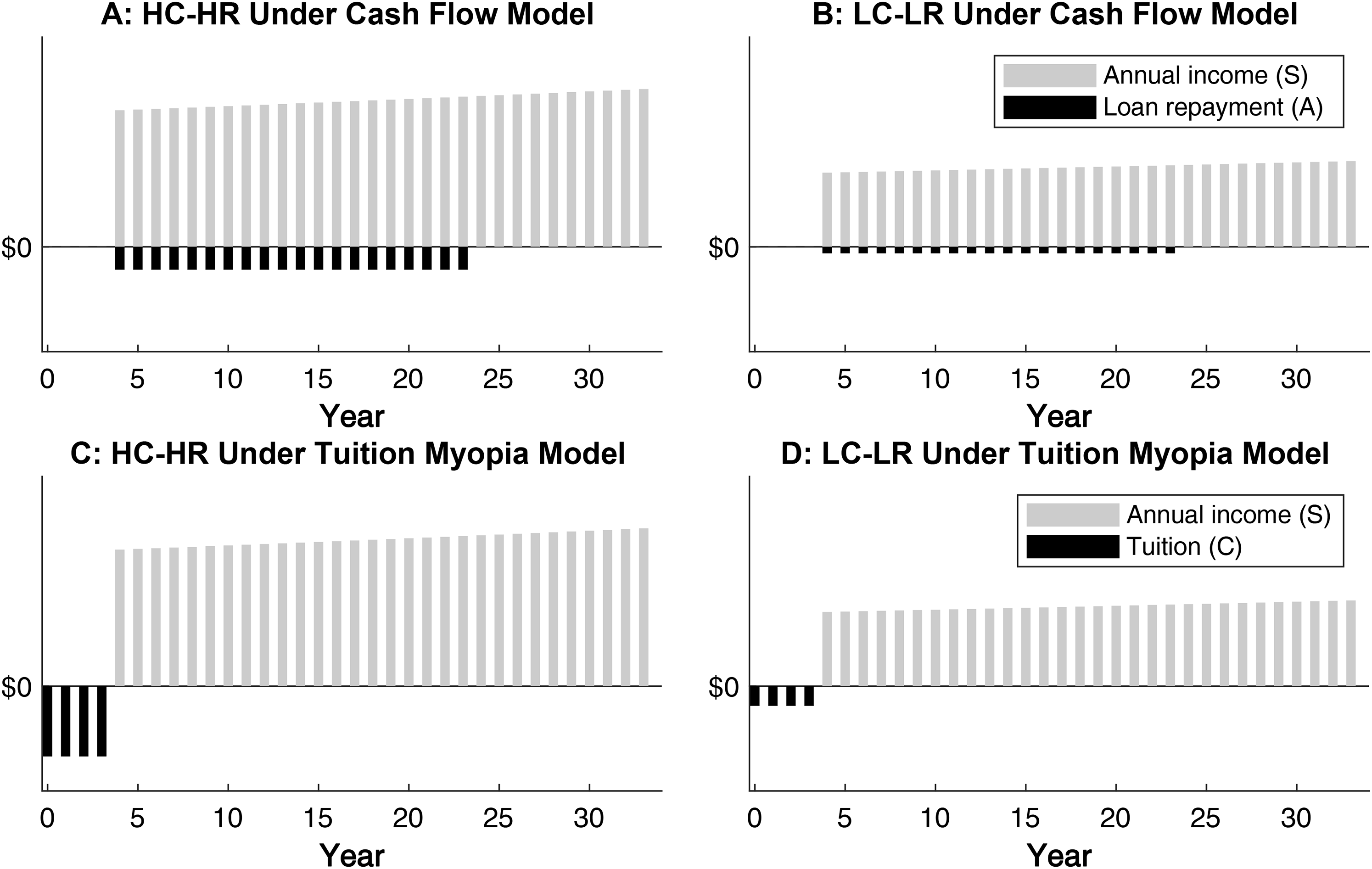
Psychological realization of college costs and returns in the cash flow model and tuition myopia model.

The cash flow model

In the United States, the federal government’s subsidized student loan program allows most students to borrow up to $57,500. Private student loans through lenders such as Sallie Mae can cover additional education expenses. Regardless of the lender, student loan payments are deferred until after graduation, when students theoretically will begin to earn an income that reflects their college education. Effectively, student loans synchronize the actual realization of the financial costs and benefits of college. If students are rational, they will psychologically realize the costs and returns of college at the same time as the costs and returns are actually realized. The financial value of a college at the time of enrolling (present value [PV]) can be estimated based on the projected cash flow after graduation:

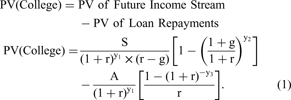
\begin{aligned} PV (College) = & PV of Future Income Stream \\ - PV of Loan Repayments \\ PV (College) = & \frac{S}{{(1 + r)}^{y_{1}} \times (r - g)} [1 - {(\frac{1 + g}{1 + r})}^{y_{2}}] \\ - \frac{A}{{(1 + r)}^{y_{1}}} [\frac{1 - {(1 + r)}^{- y_{3}}}{r}] . \end{aligned}

(1)

We assume the expected annual salary after graduation (S) will be received at the end of each working year with certainty and will grow annually at a constant rate (g). For simplicity, we assume that students are risk-neutral when evaluating the expected annual salary after graduation (S). Also, we assume that the loan interest rate (i), years spent in college (y₁), years of employment after graduation (y₂), and loan repayment period (y₃) are identical for both HC-HR and LC-LR colleges. In addition, we assume that the student pays for all college expenses using the student loan and makes annual loan repayments (A) at the end of each working year.³ The individual discount rate (r) is high for financially impatient students and low for financially patient students. With these assumptions, the present value of each college option is the present value of postgraduation income streams minus the present value of future loan repayments.

The tuition myopia model

We suggest that students do not psychologically realize costs and returns at the same time, even though student loans synchronize the actual realization of costs and returns after graduation. We ground our theory in research suggesting that the psychological temporal distance of an event depends on its valence. Negative events are often perceived as nearer than positive events, even when their objective temporal distance is the same (Bilgin and LeBoeuf 2010; Van Boven et al. 2010). A conference talk one will give in a week feels psychologically nearer, for instance, if it is dreaded than if it is eagerly anticipated. In the context of college decisions, we suggest that students psychologically realize the financial costs of college earlier than the financial returns, even though they will actually realize the costs and returns at the same time, after graduation. We refer to this misalignment as tuition myopia. If students psychologically realize the costs of college while attending but psychologically realize the returns after graduation, then the present value of a college upon enrollment is as follows:

\begin{aligned} PV (College) = & PV of Future Income Stream \\ - PV of Attendance Costs During College \\ PV (College) = & \frac{S}{{(1 + r)}^{y_{1}} \times (r - g)} [1 - {(\frac{1 + g}{1 + r})}^{y_{2}}] \\ - C (1 + r) [\frac{1 - {(1 + r)}^{- y_{1}}}{r}] . \end{aligned}

(2)

The present value of the future income stream is the same as in the cash flow model, but the present value of attendance costs during college is different. For simplicity, our tuition myopia model assumes that students psychologically realize the annual costs associated with attending a college (C) at the beginning of each school year, and those costs remain constant until graduation. All other assumptions and notations are the same as in the cash flow model.

A Choice Between an HC-HR College and an LC-LR College

The only difference between the cash flow and tuition myopia models is the timing of the psychological realization of costs, yet the models make dramatically different predictions for a choice between an HC-HR college and an LC-LR college. Under the cash flow model, the HC-HR college should dominate the LC-LR college in most choice pairs because the higher projected postgraduation cash flow compensates for the higher postgraduation loan repayments. Moreover, because both income and student loan payments are psychologically realized when they are actually realized after graduation, the individual discount rate (r) should not induce a preference reversal; the delay in the income stream is the same for HC-HR and LC-LR colleges (although the net amount is different). The decision is conceptually similar to a choice between $200 in one year and $100 in one year. The individual discount rate exerts the same influence on the present value of both colleges, so the financially dominant option is unchanged.

Under the tuition myopia model, however, the individual discount rate (r) has a significant effect on the dominant college option. The tuition myopia model posits that costs are psychologically realized before returns. Financially impatient students weigh short-term financial outcomes (costs) more heavily than long-term financial outcomes (returns), so the LC-LR college is more appealing for its lower short-term costs. Financially patient students weigh short-term financial outcomes (costs) less heavily than long-term financial outcomes (returns), so the HC-HR college is more appealing for its larger long-term returns. Thus, the tuition myopia model predicts that the dominant college option varies with the individual discount rate. For each college pair, an r_threshold exists; students below (above) the threshold should prefer the HC-HR (LC-LR) college, and students at the r_threshold should be indifferent.

We tested whether the two models indeed predict different college choices with model simulations using our exploratory data set of 83,250 HC-HR and LC-LR choice pairs from the College Scorecard database. We tested the predictions of both models under various economic parameters and assumptions. Overall, the simulation using the cash flow model predicted that the HC-HR college dominates the LC-LR college in 85.36% of the pairs regardless of the individual discount rate. The simulation using the tuition myopia model predicted that intertemporal trade-offs would determine the dominant option in 90.02% of the pairs—in other words, the individual discount rate influences a large majority of choices. For more details, see Web Appendix B.

Overview of Studies

We report seven studies that examine how students evaluate financial costs and returns when choosing between colleges. In Study 1, we measure the timing of the psychological and actual realization of the costs and returns of a college education; we also directly replicate this measurement with online and nationally representative samples. In Studies 2a and 2b, we test the predictions of the cash flow and tuition myopia models. We examine whether intertemporal trade-offs and temporal discounting influence pairwise choices between an HC-HR and LC-LR college. In Studies 3a and 3b, we test the robustness of the tuition myopia model by comparing its predictions against student debt aversion (Burdman 2005) and a strategy to maximize the ROI. We then test in Study 3c whether the model generalizes to more realistic scenarios in which students have access to a greater variety of financial and nonfinancial college information. Finally, in Study 4, we attempt to attenuate tuition myopia using an alternative presentation format that nudges students to synchronize their psychological realization of costs and returns, after graduation. We also test whether students have asymmetric beliefs about the future returns associated with LC-LR and HC-HR colleges.

Study 1

In our first test of the tuition myopia model, we measured the timing of students’ psychological realization of the financial costs and returns of a college education to determine whether there is a misalignment between psychological and actual realization. We operationalized costs and returns as College Scorecard’s projected attendance costs and postgraduation salary. Undergraduate students imagined that they received a student loan that would cover all college expenses, and they reported when the financial costs and returns of their college education would be psychologically realized and actually realized. We predicted that students would (1) psychologically realize the financial costs earlier than the financial returns, (2) psychologically realize the financial costs before their actual realization, and (3) psychologically realize the financial returns at the same time as their actual realization. We also directly replicated this study and found similar results with a convenience sample from Amazon Mechanical Turk (N = 501) and a nationally representative sample of Americans (N = 99; see Web Appendix C).

Method

Participants and exclusions

Four hundred twenty-four undergraduate students from a large nonprofit state university in the southern United States (279 women; M_age = 21.20 years, SD = 5.28 years) completed the study. As preregistered (https://aspredicted.org/blind.php?x=zj8959), we excluded 36 participants who failed an attention check, leaving a final sample of 388 participants for analyses.

Stimuli and procedure

Participants imagined that they were planning to attend a four-year college (starting in fall 2021) and use a student loan to cover all attendance costs. They were presented with financial information including the college’s annual attendance costs, the annual loan repayment amount after graduation, and the average annual salary after graduation (see Figure W8 in Web Appendix D). Next, participants reported in which year (between 2021 and 2030, inclusive) they would psychologically realize the financial costs and returns of college: “In what year would you begin to feel the financial costs of college tuition (i.e., psychologically)?” and “In what year would you begin to feel the financial benefits of college tuition (i.e., psychologically)?” Participants also reported in which year they would actually realize the financial costs and returns: “In what year would you actually start paying for the financial costs of college tuition?” and “In what year would you start receiving the financial benefits of college?” The order of the two sets of questions was counterbalanced.

Results and Discussion

A 2 (financial attributes: costs vs. returns; within-participants) × 2 (realization: psychological vs. actual; within-participants) repeated-measures analysis of variance (ANOVA) revealed significant main effects of financial attributes (F(1, 387) = 203.65, p < .001, $η_{p}^{2}$ = .35) and realization (F(1, 387) = 88.08, p < .001, $η_{p}^{2}$ = .19) in addition to the predicted significant interaction effect (F(1, 387) = 64.10, p < .001, $η_{p}^{2}$ = .14). As illustrated in Figure 2, the psychological realization of the financial costs preceded graduation (2025), when the costs would be actually realized (Mode_{psych_costs} = 2021, Median_{psych_costs} = 2022, M_{psych_costs} = 2023.05, SD = 2.22 vs. Mode_{actual_costs} = 2025, Median_{actual_costs} = 2025, M_{actual_costs} = 2024.59, SD = 1.83; t(387) = 12.01, p < .001; Wilcoxon signed-ranks test: Z = 10.37, p < .001), but the financial returns were psychologically and actually realized at the time of graduation (Mode_{psych_returns} = 2025, Median_{psych_returns} = 2026, M_{psych_returns} = 2025.48, SD = 2.86 vs. Mode_{actual_returns} = 2025, Median_{actual_returns} = 2025, M_{actual_returns} = 2025.65, SD = 2.19; t(387) = 1.34, p = .18; Wilcoxon signed-ranks test: Z = 1.07, p = .28). Moreover, the financial costs of college were psychologically realized significantly earlier than the financial returns (t(387) = 14.55, p < .001; Wilcoxon signed-ranks test: Z = 11.57, p < .001).

Figure 2.

Timing of the psychological versus actual realization of costs and returns for students enrolling in 2021 (Study 1).

Students psychologically realized the costs of college earlier than the date of their first loan repayment (i.e., actual realization) but psychologically realized the returns at the same time as when they could expect to earn an income. In short, students psychologically realized financial costs earlier than returns, providing initial support for our tuition myopia model.

Studies 2a and 2b

We next compared the predictive validity of the tuition myopia model against the cash flow model by examining preferences among choice pairs in our exploratory data set.

Our tuition myopia model predicts that people treat a choice between an HC-HR college and an LC-LR college as an intertemporal trade-off. The cash flow model predicts that people consider the projected future cash flow, so the HC-HR college should be the dominant option in most choice pairs. How can we compare these models empirically? A general preference for the LC-LR college would violate the predictions of the cash flow model but would not necessarily support the tuition myopia model. To test the tuition myopia model’s prediction regarding an intertemporal trade-off, we examined the modulation of preferences by the individual discount rate (Studies 2a and 2b) and by the threshold discount rate at the pair level (i.e., the r_threshold for each choice pair; Study 2b).

Individual-level prediction

The tuition myopia model predicts that for most choice pairs, the individual discount rate (r) determines whether the student will choose the HC-HR college or the LC-LR college. Financially impatient students (high r) should choose the LC-LR college, whereas financially patient students (low r) should choose the HC-HR college. We define r_threshold as the individual discount rate threshold at which this split should occur. All else equal, the tuition myopia model predicts that students should choose the HC-HR (LC-LR) college when their individual discount rate (r) is lower (higher) than the r_threshold of the choice pair.

Pair-level prediction

The r_threshold of the choice pair can also predict the overall choice shares of the HC-HR and LC-LR colleges. The tuition myopia model predicts that the HC-HR college should have a higher choice share in choice pairs with a high r_threshold. Only students with extremely high discount rates will have an individual discount rate that exceeds the threshold and prefer LC-LR colleges. Similarly, the LC-LR college should have a higher choice share in choice pairs with a low r_threshold. Only students with extremely low discount rates will have an individual discount rate that falls below the threshold and prefer HC-HR colleges.

In Study 2a, we tested the individual-level prediction of the tuition myopia model by measuring the relationship between the individual discount rate and real college choices. In Study 2b, we repeated the test of the individual-level prediction with hypothetical college choices, and we also tested the pair-level prediction by measuring the individual discount rate and using choice pairs with different r_threshold values.

Study 2a

In Study 2a, we tested the individual-level prediction of the tuition myopia model by examining whether the individual discount rate is related to real college choices. For each participant, we measured their individual discount rate, their highest level of education, the specific college or university they attended (if any), and basic demographic questions (i.e., gender, age, and self-reported annual income). We categorized colleges and universities as LC-LR or HC-HR using a college group ranking based on the Carnegie Classification (2015 edition), which was designed by the Indiana University Center for Postsecondary Research (Indiana University Center for Postsecondary Research 2016). The Carnegie Classification categorizes degree-granting postsecondary colleges in the United States based on years of education provided (two or four), the ratio of full-time to part-time students, the transfer-in rate, and average test scores (SAT and ACT) of admitted students. We predicted that participants with lower discount rates would be more likely to achieve a higher level of education. Moreover, among participants who attended a college, the likelihood of attending an HC-HR college should be higher among participants with lower discount rates.

Method and Design

Participants and exclusions

We recruited 600 U.S. residents from Amazon Mechanical Turk (267 women; M_age = 36.14 years, SD = 12.26 years); average self-reported individual annual income was $37,808. One participant was excluded because of a technical error, and 4 participants were excluded because of nonpositive time preferences (negative discounting or zero discounting).⁴ Of the remaining 595 participants, 4 participants had not attained a high school diploma, 81 had attained a high school diploma, 188 started but did not finish college, 261 had attained a college degree, and 61 had attained a graduate degree (Web Appendix E).

Procedure

To measure their individual discount rate, participants first completed the three-option adaptive discount (ToAD) procedure (Yoon and Chapman 2016), which asks ten intertemporal choice questions with three possible responses (e.g., “Would you prefer $7,215.77 today, $8,780.08 in 134 days, or $9,474.01 in 216 days?”) and uses an adaptive algorithm to update choice questions after each answer to estimate the individual discount rate (see Figure W9 in Web Appendix F). We programmed the ToAD procedure to present participants with intertemporal choices with an average value of $10,000 and an average delay of 182 days. Then, participants provided their demographic information, including highest level of educational attainment. Participants who had attended a college reported their alma mater.

After the experiment, we matched participants’ colleges to college financial information using the College Scorecard database and the Integrated Postsecondary Education Data System (National Center for Education Statistics). Of the 510 participants who attended college, we were able to identify the alma mater of 460 participants (representing 323 unique colleges) in both the Integrated Postsecondary Education Data System and the Carnegie Classification. We could not retrieve the information for the 47 participants who attended college outside the United States or submitted inaccurate college names, nor for three participants whose college was omitted from the Carnegie Classification. These participants were included in the educational attainment analysis but were excluded from the college choice analysis.

We used the Carnegie Classification at the undergraduate level to rank the colleges from two-year colleges to four-year, full-time, more selective, and lower transfer-in colleges. In other words, the lowest end of the ranking featured the epitome of LC-LR colleges, and the highest end featured the most HC-HR colleges. We then segmented participants into five roughly equal groups using their college rank (Web Appendix G).

Results and Discussion

Educational attainment and the individual discount rate

We examined the relationship between educational attainment and the individual discount rate for participants who had attained a high school diploma or more (n = 591). Participants who did not have a high school diploma were excluded because of the small sample size (n = 4).⁵ We found a negative relationship between the discount rate and level of educational attainment (β = −.15, t(589) = −3.79, p < .001), suggesting that financially patient people achieved a higher level of education. As a validity check, we found a positive relationship between level of educational attainment and annual income (β = .35, t(589) = 8.96, p < .001); people reporting higher levels of education reported having a higher income. There was no significant correlation between age and the individual discount rate (r = −.05, p = .16).

Validation of ranks

We validated the Carnegie Classification ranks by examining the relationship between the attendance costs and annual salary ten years after enrollment, as reported in the College Scorecard database. Enrollment is used as the reference point for postgraduation salary so that it can be compared across two-year and four-year colleges. Linear regression analysis showed that both the net attendance costs and tenth-year salary were positively related to the rank order (costs: β = .67, t(457) = 19.10, p < .001; salary: β = .74, t(454) = 23.72, p < .001),⁶ confirming that higher-ranked (vs. lower-ranked) colleges both were more expensive to attend and yielded higher income after graduation.

College choice and the individual discount rate

We used the rank order to examine the relationship between the rank of the attended college and the individual discount rate (n = 460). Figure 3 depicts the negative relationship (β = −.19, t(458) = −4.07, p < .001); that is, participants with a higher (lower) discount rate were more likely to attend a lower-ranked (higher-ranked) college.

Figure 3.

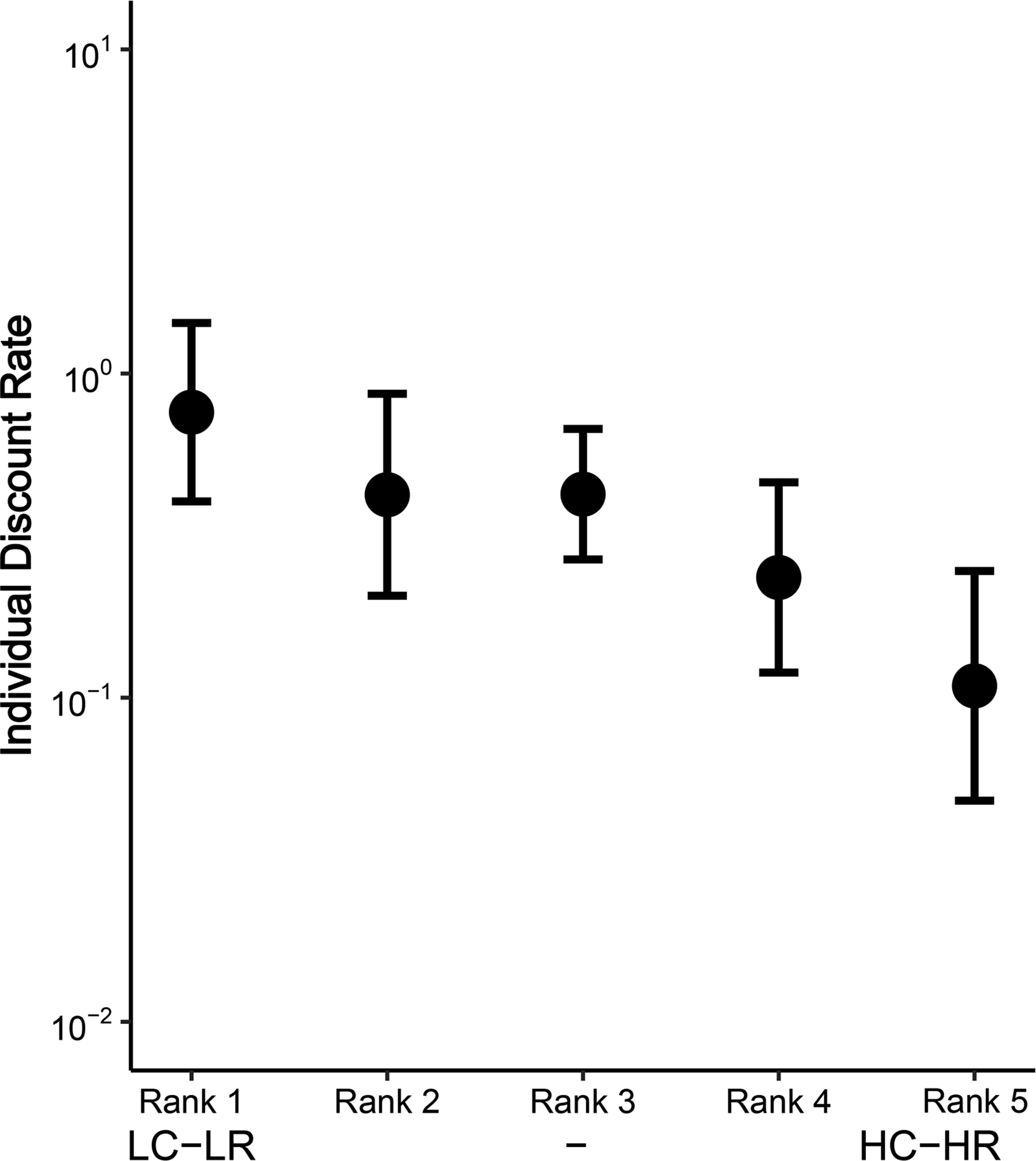
Rank of attended college by the individual discount rate in Study 2a.

The inverse relationship between the individual discount rate and rank of the attended college supports the individual-level prediction of the tuition myopia model. Replicating earlier work (Lawrance 1991; Mischel et al. 2011; Reimers et al. 2009), we also found a negative relationship between the individual discount rate and likelihood of attaining higher education; that is, participants with a lower discount rate were more likely both to have attended any college and to have completed postgraduate studies.

We note one key limitation of the cross-sectional design: We measured the individual discount rate an average of 18 years after participants had made decisions regarding their higher education. Although we did not find a correlation between age and the individual discount rate, it is possible that education and career choices influenced the discount rate in the years after the original college decision.

Study 2b

Study 2b tested both the individual-level and pair-level predictions of the tuition myopia model using hypothetical college choices. At the individual level, the model predicts that participants with a higher (vs. lower) discount rate should be more likely to choose the LC-LR (HC-HR) college in any given choice pair. At the pair level, the model predicts that the choice shares of the LC-LR and HC-HR options should depend on the r_threshold value of the choice pair; the LC-LR (HC-HR) college should have a higher choice share when r_threshold is low (high).

Method and Design

Participants and exclusions

One hundred four undergraduate business majors at a private university in New England (44 women; M_age = 20.02 years, SD = .81 years) participated for course credit. Two participants were excluded because of a technical error during the experiment. We included eight attention check questions that were similar to the main college choice questions but had an objectively dominant option—there was no trade-off between attendance costs and expected lifetime income (e.g., College A with 30-year return of $3 million and four-year costs of $100,000 vs. College B with 30-year return of $1 million and four-year costs of $100,000; College A is the financially dominant option in this example). Before the experiment, we established an exclusion criterion of three or more failed attention checks (>25% error rate), and we excluded 10 participants on this basis. The following analysis was conducted using the remaining 92 participants.

Stimuli and procedure

From the exploratory data set of 83,250 choice pairs, we randomly selected 12 choice pairs each from the 20th, 50th, and 80th percentiles (±5%) of the r_threshold values, corresponding to r_threshold values of 13.3%, 24.4%, and 42.9% annual percentage rate (APR). For each of the 36 choice pairs, participants saw the total four-year costs and 30-year expected financial returns for both colleges (Figure W10 in Web Appendix H). We estimated the individual discount rate with the ToAD procedure, borrowed from Yoon and Chapman (2016) and explained in Study 2a.

Results and Discussion

To test the individual-level prediction of the tuition myopia model, we analyzed the relationship between the individual discount rate and the choice share of the LC-LR colleges using linear regression. We found that the individual discount rate predicted the choice share of the LC-LR colleges (F(1, 90) = 12.25, p < .001, R² = .12), such that the LC-LR choice share was higher among participants with a higher individual discount rate (β = .35, t(90) = 3.5, p < .001; Figure 4, left).⁷

Figure 4.

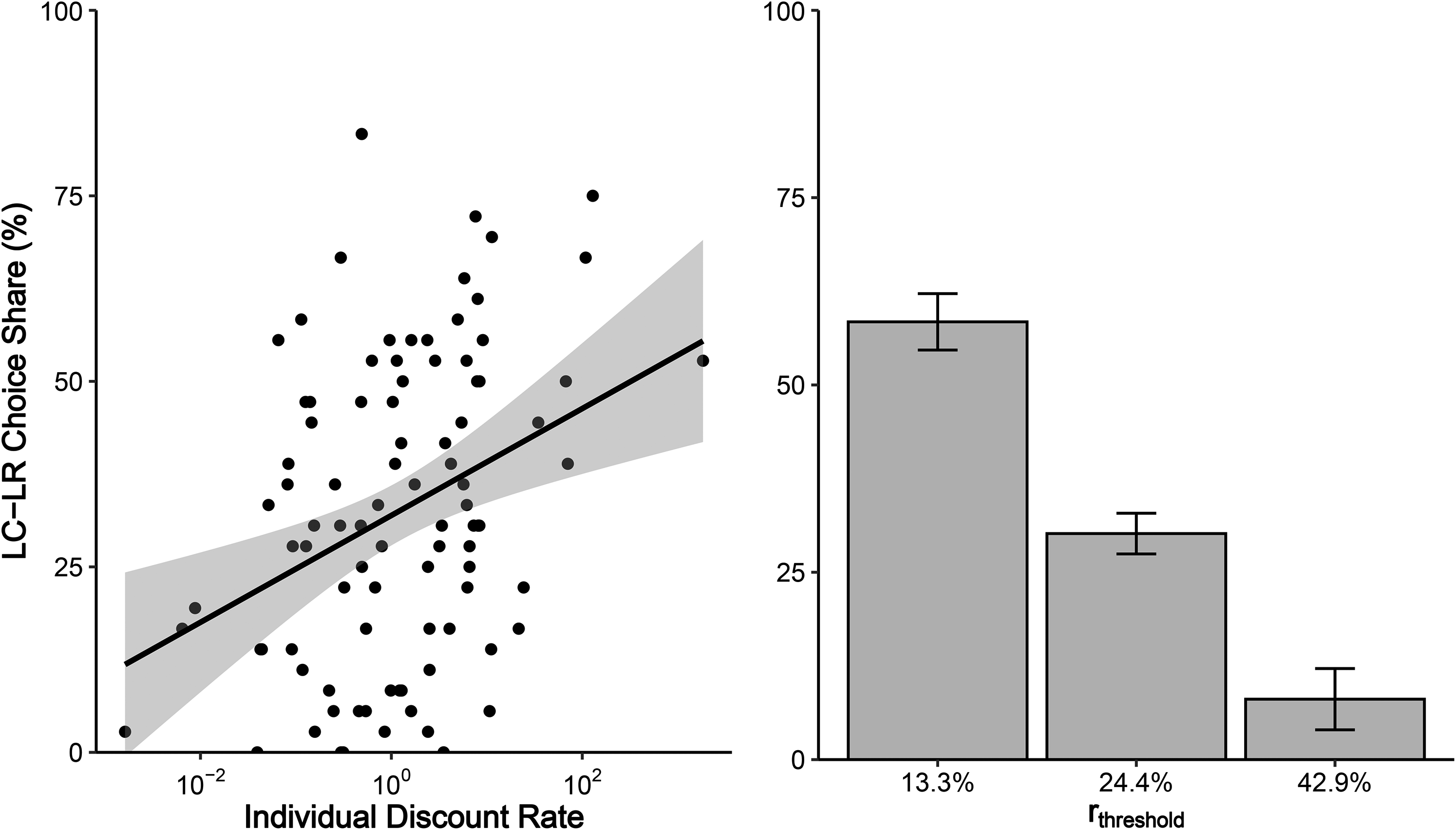
Choice share of LC-LR colleges by the individual discount rate and r_threshold in Study 2b.

To test the pair-level prediction, we examined the choice shares of the LC-LR colleges across the three r_threshold levels within participants using a repeated-measures ANOVA. For each participant, we calculated the choice share of the LC-LR colleges at each of the three r_threshold levels. For example, a participant who chose the LC-LR college in 9 of 12 choice pairs yielded a score of 75% for that cell (Figure 4, right). We found the expected significant difference between r_threshold values (F(2, 182) = 192.0, p < .001, $η_{p}^{2}$ = .68).

The results provide evidentiary support for the tuition myopia model at both levels of analysis. Supporting the individual-level prediction, financially impatient participants (i.e., those with a higher individual discount rate) were more likely to choose the LC-LR college than their less impatient peers (Figure 4, left). Supporting the pair-level prediction, participants were more likely to choose the LC-LR (HC-HR) college in choice pairs with a low (high) r_threshold (Figure 4, right).

Studies 3a, 3b, and 3c

In Studies 3a–c, we tested the robustness of the tuition myopia model by comparing its performance with plausible alternative accounts (Studies 3a and 3b) and testing the model’s generalizability to a more realistic scenario (Study 3c). In Study 3a, we compared the tuition myopia model with an ROI decision strategy, which is recommended by some for-profit and nonprofit organizations. It maximizes the ratio of net returns to costs (Lobosco 2014). In Study 3b, we compared the tuition myopia model with the theory of student debt aversion (Burdman 2005). It implies that students focus predominantly on the cost comparison within a choice pair. In Study 3c, we tested the generalizability of our model to situations in which students have access to more types of information, both financial and nonfinancial. We also varied the amount of student loan information because research on student debt aversion suggests that the provision of more details can reduce debt aversion and increase the attractiveness of the higher-cost college (Burdman 2005).

Study 3a

In Study 3a, we compared the predictions of the tuition myopia model with an investment strategy of maximizing ROI. Note that we compared two descriptive models, not two normative models, in this experiment; that is, we tested how consumers choose colleges, not how they should choose colleges. A higher ROI reflects a more efficient investment, so consumers can maximize financial portfolio returns by purchasing multiple financial assets with high ROIs. In the context of college choices, PayScale provides ROI estimates for colleges (Annual College ROI Report), and the media often cites high ROI colleges as the “best value” (Lobosco 2014). Colleges with high attendance costs (including HC-HR colleges) tend to have a low ROI (for analysis results, see Web Appendix I), so students using ROI criteria may prefer less expensive colleges (i.e., LC-LR colleges). Paradoxically, using this investment strategy could thus make their college decisions appear financially impatient. To disentangle the predictions of an ROI strategy and our tuition myopia hypothesis, we varied the r_threshold levels of the choice pairs while holding the ROI level constant, and vice versa, and examined whether the choice share is affected by the varying r_threshold levels or by varying ROI levels.

Method

Participants and exclusions

One hundred residents of the United States were recruited from Amazon Mechanical Turk (60 women; M_age = 31.26 years, SD = 9.15 years). The average self-reported annual household income was $47,239. Nine participants had attained a postgraduate degree, 39 had attained a college degree, 45 had attended college but did not have a degree, 5 had attained a GED or high school diploma, and 1 reported no degree. Two participants were excluded for failing the set of eight attention checks as described in Study 2b. One additional participant was excluded because of a technical error during the experiment. There were no other exclusions.

Stimuli and procedure

For each of the 83,250 choice pairs in the exploratory data set, we calculated the r_threshold and the ROI difference between the HC-HR and LC-LR colleges. We selected choice pairs from the 5th and 30th percentiles (±5%) of each factor, yielding average ROI differences of 6 and 45 and average r_threshold values of 4.8% and 17.2%. Participants were presented with ten choice pairs for each combination of the two factors (2 × 2 full factorial design; two ROI levels and two r_threshold levels). Each participant thus encountered 40 choice pairs and eight attention check pairs in a random order. For each college, we provided the same aggregated financial information as in Study 2b (four-year costs and 30-year returns).

Results and Discussion

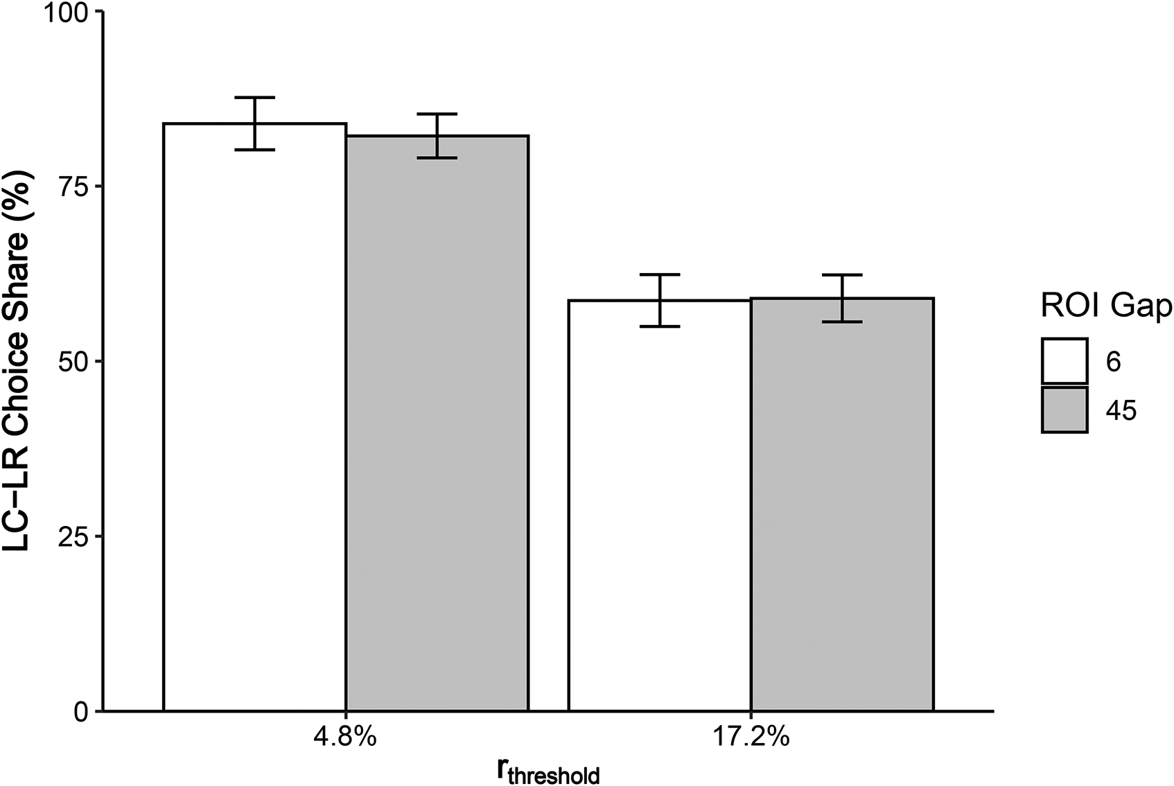
First, we calculated the choice share of the LC-LR colleges at each of the two r_threshold levels (as we did in Study 2b), split into two indices by their ROI (Figure 5). We examined the college choices in a 2 (ROI difference: 6, 45) × 2 (r_threshold APR: 4.8%, 17.2%) repeated-measures ANOVA. The analysis revealed a significant effect of r_threshold (F(1, 96) = 85.98, p < .001, $η_{p}^{2}$ = .47) but no main effect of the ROI difference (F(1, 96) = .35, p = .55) and no interaction effect between r_threshold and the ROI difference (F(1, 96) = .87, p = .35). In other words, participants were insensitive to the ROI difference but were sensitive to r_threshold, supporting the tuition myopia model and challenging the possibility that the preference for LC-LR colleges reflects the use of an ROI decision strategy. Regardless of whether ROI is an appropriate decision strategy, our results suggest that most people do not employ it when choosing which college to attend.

Figure 5.

Choice share of the LC-LR colleges by ROI difference and r_threshold in Study 3a.

Study 3b

In Study 3b, we compared whether college choices are explained more parsimoniously by our tuition myopia model or by student debt aversion (Burdman 2005), a form of loss aversion in which the student focuses disproportionately on minimizing costs (vs. maximizing benefits). Students who make decisions based on debt aversion might avoid large immediate financial expenses and ignore long-term returns entirely. To test this possibility, we constructed new choice pairs to disentangle the effects of r_threshold and the cost gap (i.e., the difference in attendance costs between the HC-HR college and the LC-LR college). We varied the r_threshold levels of the choice pairs while holding the cost gap levels constant, and vice versa, and examined whether the choice share is affected by the varying r_threshold levels or by varying cost gap levels.

Method

Participants and exclusions

Ninety-nine undergraduate business majors at a private nonprofit university in New England (45 women; M_age = 19.50 years, SD = .86 years) participated for course credit. Fifteen participants were excluded for failing the set of attention checks as described in Study 2b. There were no other exclusions.

Stimuli and procedure

We provided aggregated financial information (four-year costs and 30-year returns) for each college. For each of the 83,250 choice pairs in the exploratory data set, we calculated the cost gap and r_threshold. We randomly selected ten choice pairs at the 15th, 50th, and 85th percentiles (±4%) of each factor, yielding average cost gaps of $6,000, $24,000, and $61,000 and average r_threshold values of 11.2%, 24.1%, and 48.2% APR. We crossed the three cost gap levels with the three r_threshold levels to yield a 3 × 3 full factorial within-participants design. Each participant encountered 90 choice pairs and 8 attention check pairs in a random order on a computer.

Results and Discussion

We calculated the choice share of the LC-LR colleges in each of the nine cells, as we did in Study 2b (Figure 6), and we analyzed them in a 3 (cost gap: $6,000, $24,000, $61,000) × 3 (r_threshold: 11.2%, 24.1%, 48.2%) repeated-measures ANOVA. We found a main effect of r_threshold (F(2, 166) = 130.24, p < .001, $η_{p}^{2}$ = .61) but no main effect of the cost gap (F(2, 166) = 2.28, p = .11). The analysis showed a significant interaction between the cost gap and r_threshold (F(4,332) = 10.44, p < .001, $η_{p}^{2}$ = .11), which was largely driven by an unexpected difference between the $6,000 and $61,000 cost gap conditions at 11.2% APR (post hoc analyses using Bonferroni correction). In other words, participants did not always choose the cheaper college even at the highest cost gap level (i.e., $61,000), but they were sensitive to r_threshold. These results suggest that participants considered both proximal costs and distant gains when making college choices, in support of the tuition myopia model.

Figure 6.

Choice share of the LC-LR colleges by the cost gap and r_threshold in Study 3b.

The results from Studies 3a and 3b provide insight into students’ approach to evaluating the financial costs and returns of higher education. The results of Study 3a suggest that a focus on the ratio of returns to costs (ROI) does not explain the preference for LC-LR colleges. The results of Study 3b suggest that students consider both immediate financial costs and distant financial returns; their decisions are not driven solely by debt aversion (Burdman 2005). As predicted by the tuition myopia model, when students compare the financial costs and returns of a pair of colleges, they perceive an intertemporal trade-off, and their choices reflect the r_threshold of the choice pairs.

Study 3c

Study 3c examined whether tuition myopia extends to more realistic choice scenarios in which students consider both financial and nonfinancial college attributes, such as the school’s name (and reputation), size, location, and graduation rate. Students who have access to information about nonfinancial attributes may use a different decision strategy or ignore one or both financial attributes (e.g., frame the choice as a trade-off between costs and reputation). We manipulated the presence of these attributes by presenting participants with either the financial information alone (as in previous studies) or with a screenshot of each college’s page on the College Scorecard website, which features the same financial information as well as the college’s name, size, location, and graduation rate. In addition, we manipulated the amount of information provided about student loans (such as loan interest rate and repayment period) because a prior qualitative study suggests that student debt aversion decreases when more loan information is provided (Burdman 2005).

Method

Participants and exclusions

Three hundred twenty residents of the United States were recruited from Amazon Mechanical Turk (164 women; M_age = 36.42 years, SD = 12.67 years). Twenty-six participants were excluded for failing the set of eight attention check questions as described in Study 2b. The analysis was conducted with the remaining 294 participants.

Stimuli and procedure

The study employed a 2 (information richness: scorecard vs. financial information; between-participants) × 2 (loan information: general vs. specific; between-participants) × 3 (r_threshold: 11.8%, 21.1%, and 37.8% APR; within-participants) mixed design.

Information richness

For each college within each choice pair, participants in the financial-information conditions received only the average annual cost and salary after attending from the College Scorecard website (for examples, see Web Appendix J, Figures W12 and W13) while participants in the scorecard conditions viewed a screenshot from the College Scorecard website that featured the same financial information as well as the college’s name, size, location, and graduation rate benchmarked against the national average (for examples, see Web Appendix J, Figures W14 and W15). We retrieved the college financial information and College Scorecard screenshots in January 2017.

Loan information

In the general-loan condition, participants read, “When making your decision, please assume that there are loans available that can help you pay for the tuition and expenses required.” In the specific-loan condition, participants read, “When making your decision, please assume that you’ve already decided to take a 30-year student loan that fully covers the tuition and expenses required, regardless of which college you’ll attend. The interest rate of the student loan is 3.76%, and you’ll start repaying your student loan after you graduate from college.” (A 30-year term and 3.76% APR was the most favorable federal student loan offered from July 2016 to June 2017.)

r_threshold

From the 83,250 college choice pairs in our exploratory data set, we randomly selected 10 choice pairs each from the 20th, 50th, and 80th percentiles (±5%) of r_threshold, yielding average values of 11.8%, 21.1%, and 37.8% APR.

Results and Discussion

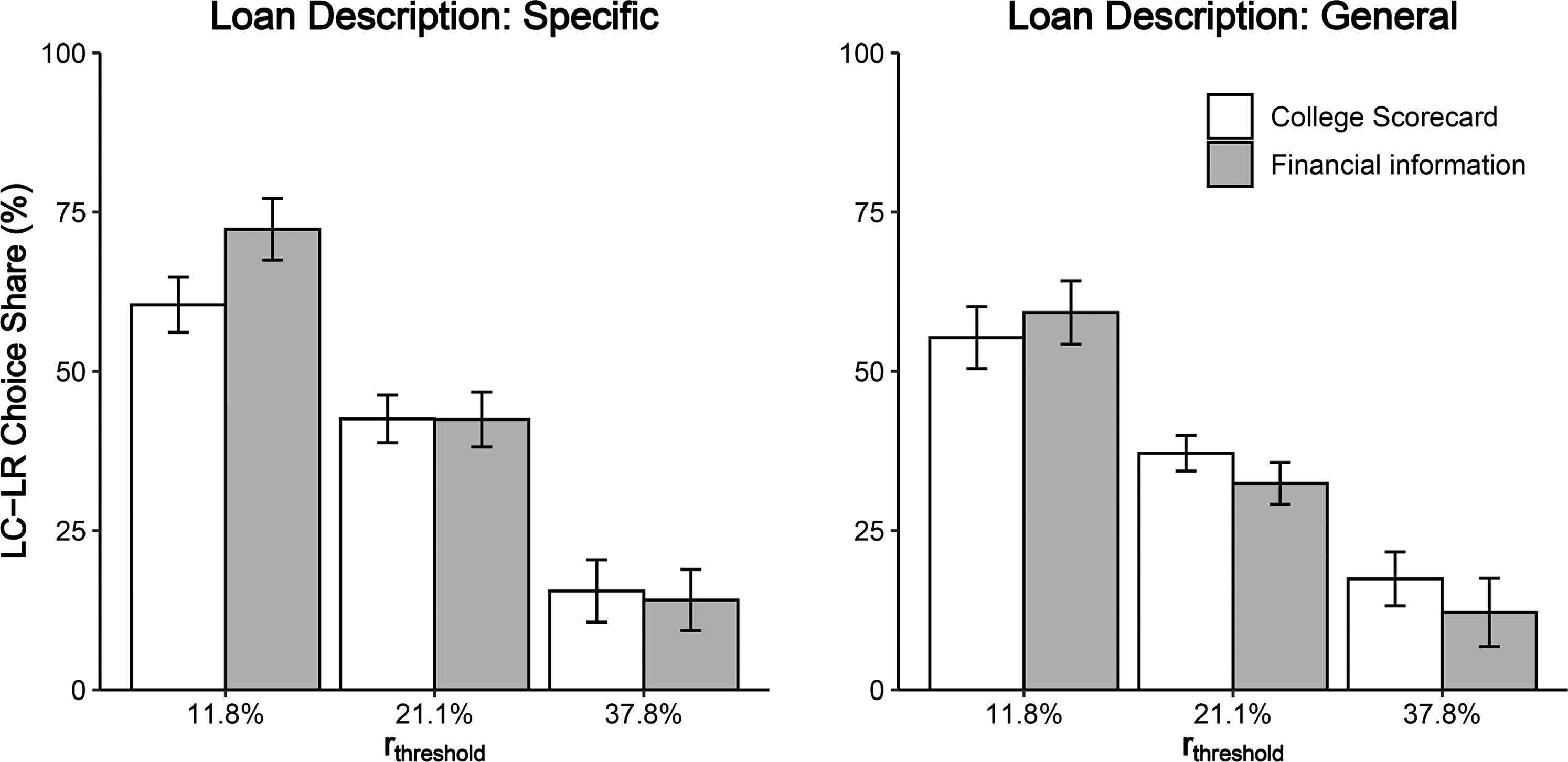
For each participant, we calculated the choice share of the LC-LR colleges at each of the three r_threshold levels, as we did in Study 2b. We then analyzed the choices in a 2 × 2 × 3 mixed ANOVA, which revealed a main effect of r_threshold (F(2, 580) = 423.95, p < .001, $η_{p}^{2}$ = .59); the LC-LR colleges had the lowest (highest) choice share at the lowest (highest) r_threshold level, and significantly more participants chose the LC-LR college than the HC-HR college at the lowest r_threshold value (Figure 7). In other words, as predicted by the tuition myopia model, intertemporal trade-offs appear to have influenced choices across all manipulations of information richness and loan information.

Figure 7.

Choice share of the LC-LR colleges by loan description, information richness, and r_threshold in Study 3c (95% confidence interval).

The main effect of information richness (scorecard vs. financial information) was not significant, F < 1, suggesting that participants based their decisions primarily on financial information even when they had access to nonfinancial information. The specific loan description directionally increased the LC-LR choice share (general vs. specific loan information: F(1, 290) = 3.88, p = .05, $η_{p}^{2}$ = .01). Notably, the finding contradicts the recommendation of Burdman (2005) to provide more loan information as a strategy for reducing student debt aversion. The analysis also revealed two unpredicted interactions with small effect sizes (r_threshold × information richness: (F(2, 580) = 7.49, p < .001, $η_{p}^{2}$ = .03; r_threshold × loan information: F(2,580) = 4.60, p < .05, $η_{p}^{2}$ = .02).

Study 4

The purpose of Study 4 was twofold. First, it tested the tuition myopia model by experimentally manipulating the timing of the psychological realization of costs. Typically, college financial information is presented such that the average annual attendance costs and expected annual salary after graduation are the information displayed (e.g., College Scorecard). We speculate that this presentation format may inadvertently lead people to psychologically realize costs earlier than returns and perceive intertemporal trade-offs in college choices. We attempted to mitigate tuition myopia by modifying the presentation format: the expected annual loan repayment (rather than attendance costs) was presented alongside the expected annual salary after graduation. The alternative presentation format presented both the costs and returns at the same time point—that is, after graduation—so we predicted that it would help synchronize the psychological realization of costs and benefits and thereby increase the choice share of the HC-HR colleges.

Study 4 also examined the influence of uncertain employment prospects, which could influence interpretations of the financial return information. In other words, whereas costs (whether presented as annual attendance costs or loan repayments) are certain, the future financial returns are not. We measured participants’ uncertainty about their future employment prospects after graduation from each college to see whether uncertainty reduces the attractiveness of the HC-HR college by undermining confidence in its superior returns.

Method

Participants and exclusions

We requested 200 United States residents from Prolific, and 200 participants completed the experiment (106 women; M_age = 32.97 years, SD = 14.06 years). We included three attention check questions of the type described in Study 2b; following our study preregistration (https://aspredicted.org/blind.php?x=dc4w9 g), we excluded 20 participants who failed one or more questions. The following analysis was conducted with the remaining 180 participants.

Stimuli and procedure

The study employed two conditions (cost information: annual attendance costs vs. annual loan repayment amount; between-participants). Participants imagined that they were in their senior year of high school and were deciding which four-year college to attend. They imagined that they had already decided to take out a 20-year student loan (interest rate: 4.37%) that would fully cover the tuition and expenses, regardless of which college they would attend.

We used the same ten choice pairs from Study 3c at the 11.8% r_threshold level. For each choice pair, participants received financial information (average annual salary after graduation and either the annual attendance costs or annual loan repayment amount, depending on condition; Web Appendix K, Figure W16 and W17). The annual loan repayment amount was calculated using a 20-year fixed monthly payment plan (the median loan repayment period; National Center for Education Statistics 2018) with 4.37% APR, the average federal student loan interest rate from July 2013 to June 2020. After making a choice for each choice pair, participants estimated their employment prospects after graduating from each college (“How likely is it that you would be employed within 1 year of graduating from [college above]?” 0 = “Highly unlikely,” and 100 = “Highly likely”).

Results and Discussion

First, we examined whether the presentation of cost information (format: annual attendance costs vs. annual loan repayment amount) influenced college choices. For each participant, we calculated the choice share of the LC-LR colleges, as we did in Study 2b. An independent samples t-test revealed that participants who received the annual loan repayment amount (vs. annual attendance costs) exhibited a significantly lower LC-LR choice share (M_{annual repayment} = 45.38%, SD = 34.22; M_{annual attendance} = 72.25%, SD = 30.25; t(178) = 5.57, p < .001, d = .83).

Next, we examined whether expectations about employment prospects varied with the college type and cost information. A 2 (format: annual attendance costs vs. annual loan repayment amount; between-participants) × 2 (college: HC-HR vs. LC-LR; within-participants) mixed ANOVA revealed no significant main effect of college type (F(1, 178) = .36, p = .55), no significant main effect of format (F(1, 178) = 3.10, p = .08), and no interaction effect (F(1, 178) = .003, p = .96; M_{attendance_HC-HR} = 62.87, SD = 16.17; M_{attendance_LC-LR} = 62.54, SD = 16.30; M_{repayment_HC-HR} = 66.87, SD = 14.97, M_{repayment_LC-LR} = 66.59, SD = 15.46). In other words, perceived employment prospects were not affected by the type of college or cost information presented.

The results provide insight into a method for reframing the way students consider the financial ramifications of college. Participants who were nudged to psychologically realize the financial costs and returns at the same time––after graduation, when both the costs and returns would be actually realized––were less likely to choose the LC-LR college over the HC-HR college. We also found that participants’ uncertainty about future job prospects did not differ between LC-LR and HC-HR colleges, so tuition myopia cannot be explained by a perception that future salaries are more uncertain for graduates of HC-HR colleges.

General Discussion

In the second quarter of 2010, for the first time in history, student debt surpassed auto loans and credit cards to become the second-largest source of consumer debt in the United States. Government, nonprofit, and for-profit agencies now provide college financial information in a variety of formats and advise students and their families to consider the financial ramifications of their college choices. We present an empirically supported model of the financial decision-making process by which students weigh these financial costs and returns. Our tuition myopia model provides insights into and predictions for a choice that profoundly influences one’s lifetime income. Our model also suggests an approach to the presentation of financial information that can help students attempt to maximize their lifetime income.

We began by testing two different models of the college decision process. A rational cash flow model considers the expected cash flows of costs (i.e., loan repayments) and returns (i.e., income) at the time of their actual realization (i.e., after graduation). The cash flow model predicts a preference for the HC-HR college over the LC-LR college in most choice pairs, regardless of the financial impatience of the student. In our tuition myopia model, however, the student psychologically realizes the costs before the returns, creating the perception of an intertemporal trade-off between short-term losses and long-term gains. A student’s choice between an HC-HR college and an LC-LR college depends on the relationship between the individual discount rate and the r_threshold value of the choice pair.

We find considerable evidentiary support for our tuition myopia model. In Study 1, students (and others) psychologically realized the financial costs of college earlier than the financial returns (see also Web Appendix C). In Study 2a, a retrospective analysis of real college decisions found that, among adults who previously attended college, those who were more (less) financially impatient were more likely to have attended an LC-LR (HC-HR) college. In Study 2b, we systematically varied the discount rate threshold of the choice pair (r_threshold) and found that individual-level and pair-level trends exhibited an intertemporal trade-off, as predicted by the tuition myopia model and in conflict with the predictions of the cash flow model. Studies 3a and 3b suggest that tuition myopia cannot be explained by an ROI maximization strategy or student debt aversion (Burdman 2005). In Study 3c, the tuition myopia model generalized to choice pairs for which both nonfinancial and financial attributes were available. Finally, Study 4 demonstrated that a modified decision aid can diminish tuition myopia by synchronizing the psychological realization of costs and returns.

Theoretical Contributions

Our tuition myopia model contributes primarily to the literature examining intertemporal choices for higher education. That literature has largely focused on how students decide whether to go to college. The decision is framed as a choice between a smaller, sooner reward (i.e., get a job after high school to receive income immediately) and a larger, later reward (i.e., go to college and secure a higher-paying job after graduation; Lawrance 1991; Mischel et al. 2011; Reimers et al. 2009). We extend the scope of the literature by examining intertemporal choices between colleges. Students who decide to attend college are postponing their income regardless of the specific college, so there is no “smaller, sooner” or “larger, later” reward. Public and private loans allow students to postpone work and income so they can earn a larger salary and pay back their loans after graduation, regardless of the college they choose. If students psychologically realize the financial costs and returns at the time of their actual realization (i.e., after graduation), as posited by the rational cash flow model, then there should be no intertemporal trade-off.

With correlational and experimental data, however, we show that the psychological realization of costs before returns creates the perception of an intertemporal trade-off when the choice involves a smaller short-term investment that should produce a smaller long-term return (LC-LR) and a larger short-term investment that should produce a larger long-term return (HC-HR). We propose and test a quantitative model, and we overcome a limitation of previous research in this area by explicitly demonstrating intertemporal trade-offs (Rick and Loewenstein 2008; Urminsky and Zauberman 2015).

Scope and Limitations

Readers are likely to note the discrepancy between the rising student debt burden and our implicit prescriptive advice that it is often better for students to take on more debt, but our perspective is supported by loan default data from the Consumer Financial Protection Bureau (Chopra 2013). The student loan literature continues to argue that students take on too little debt, particularly when coming from low-income and underrepresented backgrounds. Many students miss out on greater lifetime earnings by attending cheaper colleges (e.g., Avery and Turner 2012; Burdman 2005). Students with the highest student loan debt burdens are also not necessarily those who are most likely to default on their student loans or fail to complete college. Loan default rates are highest among people who were already struggling with other forms of debt payments before they took out a student loan: students with less wealth, income, and resources (Cottom 2017). Taking out too little in student loans to finance their college education may compound these pressures. They may be forced to finance their education and other expenses with more expensive credit cards or take on jobs during college that interfere with their coursework.

We recognize that the thought of a choice between an LC-LR college and an HC-HR college may conjure a mental image of choosing between a public not-for-profit university and an expensive elite private university—ostensibly an uncommon choice. In reality, about two-thirds of the choice pairs of U.S. institutions (including public not-for-profit, private not-for-profit, and private for-profit institutions) involve a choice between an HC-HR college and an LC-LR college. The terms “HC-HR” and “LC-LR” merely imply that one institution both costs more and returns more than the other, not that it is prohibitively expensive or outrageously advantageous for one’s career. The designations are relative within the choice pair, so any student who receives more than two acceptances can choose an HC-HR option if there is no financially dominant option (i.e., LC-HR option). Whether it is an Ivy League school or the nearest nonprofit public university, an HC-HR option should still yield more lifetime earnings than the LC-LR alternative for most students in the long term.

Our model’s predictions rest on four assumptions: (1) student loans eliminate immediate budgetary constraints, (2) students can obtain loans at the same interest rate regardless of the four-year attendance costs and the student’s economic background, (3) the expected annual income after graduation is certain and the same for all students, and (4) students will graduate from the college they attend. Obviously, these assumptions do not hold in all cases. The first assumption may not hold for students with little income or wealth, who may need to use student loans to pay for not only college costs but also immediate expenses such as car repairs and family emergencies. For-profit colleges tend to estimate higher costs and thus enable students to receive larger loan disbursements, so they may be the only realistic option for students with immediate financial needs beyond college costs (Cottom 2017).

Regarding the second assumption, students may not be able to cover all attendance costs with a single type of loan, so the effective interest rate may vary depending on the total four-year costs and the student’s credit history. At the college level, undergraduate students may borrow up to $57,500 in fixed-rate federal student loans, but many students need to supplement with private loans, which come with higher interest rates. Thus, the effective interest rate depends on the composition of the student’s loan package. For the same student, the loan package may differ between an LC-LR college and an HC-HR college—the lower costs of an LC-LR college may enable a student to take on only low-rate federal loans, while the same student may need to supplement with higher-rate private loans to afford an HC-HR college. At the student level, the interest rates of private loans vary with the credit history of the student or guarantor. Students whose families have low income or wealth may have to pay a higher interest rate to finance college; again, this will be disproportionately costly for the HC-HR college if private loans constitute a higher proportion of the student’s loan package. It also is worth noting variations in transaction costs, which are not part of our model. Institutions vary in the effective transaction costs for enrolling and securing a loan. For-profit universities tend to streamline the enrollment and loan process. For working adults, the transaction utility offered by a for-profit institution might outweigh the lower costs or greater financial returns they would receive from a more traditional nonprofit public or private college with more complex enrollment and loan processes (Cottom 2017).

Regarding the third assumption, the anticipated returns from any given college vary with the student’s career goals and undergraduate major. Students who pursue technical undergraduate majors, like computer science and engineering, tend to earn significantly more over their lifetimes than students who pursue a major in education or the humanities. The relative benefits of an LC-LR college may increase for students pursuing less lucrative careers. There is also considerable individual heterogeneity even within majors (Avery and Turner 2012). Students who are risk-averse or have a strong conviction that they will pursue a less lucrative career may assume they will earn less than the amount forecasted by College Scorecard and other decision aids.

The fourth assumption, that all matriculating students will graduate, is clearly untrue. Approximately half of all students who pursue a bachelor’s degree will leave college with no degree. Incompletion rates are substantially lower at not-for-profit (vs. for-profit) institutions, but the rate is nontrivial for all colleges (Avery and Turner 2012). Men and students of underrepresented minoritized groups, particularly Black students, are at the highest risk of not completing an undergraduate degree (DiPrete and Buchmann 2006; McDaniel et al. 2011). In short, depending on the student’s demographics and the type of institution under consideration, it may be appropriate to discount the forecasted financial benefits of a college, which increases the attractiveness of the LC-LR option.

Policy and Practical Implications

Our tuition myopia model can explain and predict how students consider the financial ramifications of higher education, a decision that drives the second-largest source of consumer debt in America and affects millions of students every year. Our research benefits policy makers who are attempting to design policies and interventions to help students realize their goals. It is laudable that government, nonprofit, and for-profit agencies are providing college financial information to the general public. We discover that the way in which financial information is presented can steer students toward a decision frame in which college choices seem to pose intertemporal trade-offs. As we show in Study 4, the common practice of displaying the attendance costs and expected postgraduation salary side by side may inadvertently prompt students to psychologically realize costs earlier than benefits, evoking the perception of an intertemporal trade-off in college choices that do not actually involve an intertemporal trade-off. When combined with temporal discounting and financial impatience, the most common form in which this financial information is presented increases the likelihood that students will choose the LC-LR college over the HC-HR college. We hope our findings guide the data-driven development of more effective decision aids and nudges to help students understand the financial attributes of their options for higher education and better align their decisions with personal and financial goals.

Although lifetime postgraduation gains are greater for the HC-HR college than for the LC-LR college, even when considering the higher attendance costs and larger loan repayments, we are agnostic about whether preferences for the LC-LR college are unjustified. We envision that the LC-LR college may be the better choice for a student whose aversion to greater debt imposes a psychological cost (e.g., pain of paying) that offsets greater expected financial benefits, who wants to maximize their ROI, who has the capital to invest in more profitable assets than higher education, or who would need to take on loans with a high interest rate. Admittedly, it is counterintuitive to recommend HC-HR colleges when student loans have become such a large burden for many Americans, but we find that graduates from LC-LR colleges are more likely to default on their student loans (Web Appendix L), implying that the minimization of student debt may not necessarily ensure future financial security. Considerably more work is needed to understand not only the psychology of the financial decision-making process for higher education but also the economic ramifications of those decisions in the context of the opportunity costs, considering the many boundary conditions we have identified.

It is important to understand sources of consumer debt that constrain consumers and society. It is equally important to understand the downside of underinvestment in human capital, which can lead to larger financial disadvantages in the future. A college education is a one-time opportunity for most students. Focusing on maximizing total lifetime income rather than investment efficiency may make more sense for many who wish to use this powerful ladder for economic benefit.

Footnotes

Associate Editor

Ravi Dhar

Acknowledgments

The authors thank Abby Shafroth for thoughtful comments. This research was supported in part by Lilly Endowment, Inc., through its support for the Indiana University Pervasive Technology Institute for providing supercomputing.

Declaration of Conflicting Interests

The author(s) declared no potential conflicts of interest with respect to the research, authorship, and/or publication of this article.

Funding

The author(s) received no financial support for the research, authorship, and/or publication of this article.

ORCID iDs

Haewon Yoon

Carey K. Morewedge

Online supplement:

Notes

References

Avery

Christopher

Turner

Sarah

(2012), “Student Loans: Do College Students Borrow Too Much—Or Not Enough?” Journal of Economic Perspectives, 26 (1), 165–92.

Baum

Sandy

O’Malley

Marie

(2003), “College on Credit: How Borrowers Perceive Their Education Debt,” Journal of Student Financial Aid, 33 (3), 7–21.

Becker

Gary S

. (1962), “Investment in Human Capital: A Theoretical Analysis,” Journal of Political Economy, 70 (5), 9–49.

Bilgin

Baler

LeBoeuf

Robyn A.

(2010), “Looming Losses in Future Time Perception,” Journal of Marketing Research, 47 (3), 520–30.

Burdman

Pamela

(2005), “The Student Debt Dilemma: Debt Aversion as a Barrier to College Access,” Center for Studies in Higher Education, University of California, Berkeley.

Caetano

Gregorio

Patrinos

Harry Anthony

Palacios

Miguel

(2011), “Measuring Aversion to Debt: An Experiment Among Student Loan Candidates,” Policy Research Working Paper, World Bank.

Callender

Claire

Jackson

Jonathan

(2005), “Does the Fear of Debt Deter Students from Higher Education?” Journal of Social Policy, 34 (4), 509–40.

Carr

Peggy G

. (2015), The Condition of Education 2015. Washington, DC: National Center for Education Statistics.

Chopra

Rohit

(2013), Student Debt Swells, Federal Loans Now Top a Trillion. Washington, DC: Consumer Financial Protection Bureau.

10.

Cottom

Tressie McMillan

(2017), Lower Ed: The Troubling Rise of For-Profit Colleges in the New Economy. New York: The New Press.

11.

DiPrete

Thomas A.

Buchmann

Claudia

(2006), “Gender-Specific Trends in the Value of Education and the Emerging Gender Gap in College Completion,” Demography, 43 (1), 1–24.

12.

Federal Reserve Bank of New York (2021), Quarterly Report on Household Debt and Credit 2021: Q2. New York: Center for Microeconomic Data.

13.

Federal Reserve Board (2020), Report on the Economic Well-Being of U.S. Households in 2019, Featuring Supplemental Data from April 2020. Washington, DC: Federal Reserve Board.

14.

Field

Erica

(2009), “Educational Debt Burden and Career Choice: Evidence from a Financial Aid Experiment at NYU Law School,” American Economic Journal: Applied Economics, 1 (1), 1–21.

15.

Indiana University Center for Postsecondary Research (2016), The Carnegie Classification of Institutions of Higher Education, 2015 ed. Bloomington: Indiana University Center for Postsecondary Research.

16.

Koopmans

Tjalling C

. (1960), “Stationary Ordinal Utility and Impatience,” Econometrica, 28 (2), 287–309.

17.

Lawrance

Emily C

. (1991), “Poverty and the Rate of Time Preference: Evidence from Panel Data,” Journal of Political Economy, 99 (1), 54–77.

18.

Lobosco

Katie

(2014), “Colleges That Offer the Best Return on Your Investment,” CNN Money (March 26), https://money.cnn.com/2014/03/26/pf/college/college-return-investment/index.html.

19.

McDaniel

Anne

DiPrete

Thomas A.

Buchmann

Claudia

Shwed

Uri

(2011), “The Black Gender Gap in Educational Attainment: Historical Trends and Racial Comparisons,” Demography, 48 (3), 889–914.

20.

Mischel

Walter

Ayduk

Ozlem

Berman

Marc G.

Casey

B.J.

Gotlib

Ian H.

Jonides

John

, et al. (2011), “‘Willpower’ over the Life Span: Decomposing Self-Regulation,” Social Cognitive and Affective Neuroscience, 6 (2), 252–56.

21.

National Center for Education Statistics (2018), Repayment of Student Loans as of 2015 Among 1995–96 and 2003–04 First-Time Beginning Students. NCES 2018-410. Washington, DC: U.S. Department of Education, National Center for Education Statistics.

22.

National Student Loan Data System (2021), “Federal Student Aid Portfolio Summary,” U.S. Department of Education.

23.

Reimers

Stian

Maylor

Elizabeth A.

Stewart

Neil

Chater

Nick

(2009), “Associations Between a One-Shot Delay Discounting Measure and Age, Income, Education and Real-World Impulsive Behavior,” Personality and Individual Differences, 47 (8), 973–78.

24.

Rick

Scott

Loewenstein

George

(2008), “Review. Intangibility in Intertemporal Choice,” Philosophical Transactions of the Royal Society B: Biological Sciences, 363 (1511), 3813–24.

25.

Rothstein

Jesse

Rouse

Cecilia E.

(2011), “Constrained After College: Student Loans and Early-Career Occupational Choices,” Journal of Public Economics, 95 (1/2), 149–63.

26.

Sallie

Mae

(2017), How America Pays for College 2017. Newark, DE: Sallie Mae.

27.

Samuelson

Paul A

. (1937), “A Note on Measurement of Utility,” Review of Economic Studies, 4 (2), 155–61.

28.

Schultz

Theodore W

. (1961), “Investment in Human Capital,” American Economic Review, 51 (1), 1–17.

29.

Urminsky

Oleg

Zauberman

Gal

(2015), “The Psychology of Intertemporal Preferences,” in The Wiley Blackwell Handbook of Judgment and Decision Making, Wu

George

Keren

Gideon

, eds. Hoboken, NJ: John Wiley & Sons, 141–81.

30.

U.S. Bureau of Labor Statistics (2016a), Consumer Price Index for All Urban Consumers: All Items (CPIAUCSL). Washington, DC: U.S. Bureau of Labor Statistics.

31.

U.S. Bureau of Labor Statistics (2016b), Consumer Price Index for All Urban Consumers: College Tuition and Fees (CUSR0000SEEB01). Washington, DC: U.S. Bureau of Labor Statistics.

32.

U.S. Bureau of the Census (2016), Real Median Household Income in the United States (MEHOINUSA672N). Suitland, MD: U.S. Bureau of the Census.

33.

Van Boven

Leaf

Kane

Joanne

Peter McGraw

Dale

Jeannette

(2010), “Feeling Close: Emotional Intensity Reduces Perceived Psychological Distance,” Journal of Personality and Social Psychology, 98 (6), 872–85.

34.

The White House (2013), “Remarks by the President in the State of the Union Address,” Office of the Press Secretary, news release (February 12).

35.

The White House (2015), “Fact Sheet: Empowering Students to Choose the College That Is Right for Them,” Office of the Press Secretary, news release (September 12).

36.

Yoon

Haewon

Chapman

Gretchen B.

(2016), “A Closer Look at the Yardstick: A New Discount Rate Measure with Precision and Range,” Journal of Behavioral Decision Making, 29 (5), 470–80.

Supplementary Material

Please find the following supplemental material available below.

For Open Access articles published under a Creative Commons License, all supplemental material carries the same license as the article it is associated with.

For non-Open Access articles published, all supplemental material carries a non-exclusive license, and permission requests for re-use of supplemental material or any part of supplemental material shall be sent directly to the copyright owner as specified in the copyright notice associated with the article.

0.00 MB

2.45 MB

1.64 MB

Early Cost Realization and College Choice

Abstract

Keywords

Theoretical Development

Kinds of College Choices

Two Models of College Choice

The cash flow model

The tuition myopia model

A Choice Between an HC-HR College and an LC-LR College

Overview of Studies

Study 1

Method

Participants and exclusions

Stimuli and procedure

Results and Discussion

Studies 2a and 2b

Individual-level prediction

Pair-level prediction

Study 2a

Method and Design

Participants and exclusions

Procedure

Results and Discussion

Educational attainment and the individual discount rate

Validation of ranks

College choice and the individual discount rate

Study 2b

Method and Design

Participants and exclusions

Stimuli and procedure

Results and Discussion

Studies 3a, 3b, and 3c

Study 3a

Method

Participants and exclusions

Stimuli and procedure

Results and Discussion

Study 3b

Method

Participants and exclusions

Stimuli and procedure

Results and Discussion

Study 3c

Method

Participants and exclusions

Stimuli and procedure

Information richness

Loan information

rthreshold

Results and Discussion

Study 4

Method

Participants and exclusions

Stimuli and procedure

Results and Discussion

General Discussion

Theoretical Contributions

Scope and Limitations

Policy and Practical Implications

Footnotes

Associate Editor

Acknowledgments

Declaration of Conflicting Interests

Funding

ORCID iDs

Notes

References

Supplementary Material

r_threshold