Uncovering the Spatial Patterning of Crimes

Abstract

Objectives:

The main objective of this study was to see if the characteristics of offenders’ crimes exhibit spatial patterning in crime neutral areas by examining the relationship between simulated travel routes of offenders along the physical road network and the actual locations of their crimes in the same geographic space.

Method:

This study introduced a Criminal Movement model (CriMM) that simulates travel patterns of known offenders. Using offenders’ home locations, locations of major attractors (e.g., shopping centers), and variations of Dijkstra’s shortest path algorithm we modeled the routes that offenders are likely to take when traveling from their home to an attractor. We then compare the locations of offenders’ crimes to these paths and analyze their proximity characteristics. This process was carried out using data on 7,807 property offenders from five municipalities in the Greater Vancouver Regional District (GVRD) in British Columbia, Canada.

Results:

The results show that a great proportion of crimes tend to be located geographically proximal to the simulated travel paths with a distance decay pattern characterizing the distribution of distance measures. Conclusion: These results lend support to Crime Pattern Theory and the idea that there is an underlying pattern to crimes in crime neutral areas.

Keywords

crime attractor crime pattern theory journey to crime target selection road network

Introduction

The built environment plays a major role in the daily activities of criminals and noncriminals alike. Physical structures such as houses and buildings concentrate a great deal of the activities people participate in everyday including work, school, recreation, social activities, and sleep. Similarly, the road network is a component of the built environment that facilitates movement between these locations and concentrates human activity. Some activity nodes become important areas of focus with respect to crime because they attract criminally motivated people.

Crime attractors draw offenders to specific locations because there are known criminal opportunities that exist (Brantingham and Brantingham 1995). There has been considerable evidence that a disproportionate amount of crime concentrates at or near these attractor locations (see, e.g., Block and Block 1995; Eck, Clarke, and Guerette 2007; Sherman, Gartin, and Buerger 1989). While the sheer concentration of crime makes these places important to study, they may also share an important relationship with the spatial distribution of crimes committed outside the immediate vicinity of attractors. This relationship is driven by the premise that in order to get to attractors, offenders will travel through neighborhoods, thereby increasing their awareness of other criminal opportunities that exist.

These areas, termed crime neutral, have been defined as areas where crimes are more sporadically dispersed (Brantingham and Brantingham 1995). Greatly different from hot spots (places where crimes concentrate spatially at a point in time) and cold spots (places characterized by a distinct lack of crime at a point in time), crime neutral areas may not reveal any clear spatial pattern when mapped or presented in another visual format. The tenets of Crime Pattern theory (Brantingham and Brantingham 1993), however, suggest that an underlying structure should exist. Because the target selection behavior of offenders is influenced by their activity and awareness spaces, major activity nodes and the paths that are used to navigate between them play a central role in defining where crimes will be committed (Brantingham and Brantingham 1993). With respect to crime neutral areas, specifically, offenders will develop awareness spaces along the travel paths between their major activity nodes. As a result, it is expected that offenders will develop awareness for criminal opportunities along these routes including those between offenders’ homes and major shopping centers. For example, individuals traveling from their home to a major activity node such as a shopping center may recognize opportunities for theft at strip malls and standalone stores or break and enter (burglary) residential houses along the way. It could be expected that offenders will commit crimes along or near these routes if such opportunities for crime are recognized.

The analysis of travel patterns on road networks has been used to research a variety of different routing problems in other disciplines. For example, simulation models have been used to address efficient ambulance routing (Derekenaris et al. 2001), optimal timber haulage routes (Devlin, McDonnell, and Ward 2008), and commuter traffic queries (Engelson 2003). Using real-time traffic information and geographic information system GIS data, these studies created simulation models of their specific road networks. In order to minimize travel time or travel distance in such case studies, a shortest path algorithm was used (Dijkstra 1959; Dreyfus 1960; Van Vliet 1978; Zhan and Noon 1998).

Few simulations of this type have been applied in the field of criminology. A major barrier to this research is the inability to obtain data that would make it possible to simulate the actual travel routes of known criminals. Without GPS tracking or a similar form of geographic data collection, it is difficult to obtain detailed information about the activity spaces of known criminals. Through the use of computational techniques, mathematical algorithms, and basic geographical data, it is possible to create simulated travel routes. For example, with knowledge of a likely starting point and destination, such as an offender’s home location as the start and their offending location as the destination, it is possible to calculate the route a person might take to get to their destination if they tried to minimize the distance or time it took to travel along the extant road network.

There have been a small number of studies that have employed functional distance measures for research on the travel patterns of specific types of offenders (see, e.g., Kent, Leitner, and Curtis 2006). Such studies, however, were conducted primarily for research on geographic profiling of serial offenders. We are not aware of any research that has used shortest distance and quickest time algorithms to simulate the travel patterns of known criminals for the purposes of investigating the relationship between travel routes to crime attractors and actual locations of crimes perpetrated by offenders.

In the current project, we introduce a Criminal Movement Model (CriMM) that simulates the likely routes that offenders may take when traveling from their home to a major attractor location. The objectives of the research project are to: 1) experiment with algorithms to create possible routes from offenders’ homes to activity node locations; 2) consider the relationships between these simulated travel paths, specific attractor locations, and known crime patterns in the study area; and 3) investigate the characteristics of those trips in relation to the actual locations of the crimes using a variety of proximity measures. Through these objectives, the goal is to interpret the results in relation to Crime Pattern Theory to see if the characteristics of offenders’ crimes exhibit spatial patterning in crime neutral areas.

Crime Pattern Theory and Geometry of Crime

The foundation that informs the design of the model proposed in this article is Crime Pattern theory (Brantingham and Brantingham 1993). The central idea divulged from this framework is that crime is a patterned phenomenon with respect to its spatial and temporal characteristics. Key concepts used to explain crime as a patterned event are closely connected with theories in Behavioral Geography. Many of these theories focus on the connections between human cognition, spatial decision-making, and human movements in the physical environment (see Argent and Walmsley 2009; Golledge, Neil, and Paul 2001).

There are a variety of factors that influence the way an individual maneuvers in the environment during the course of carrying out their routine activities. Personal mobility, transportation options, and the physical structure of the city are three examples of factors that may affect how a person moves from one place to the next. It has been argued that “mental maps” play an instrumental role in human movement through urban areas. Mental maps are characterized by several basic elements that include nodes (urban focal points such as recreation centers and shopping centers), paths (roads and walkways), edges (railway lines, shorelines, and physical boundaries), districts (defined areas, neighborhoods, and communities), intersections, and landmarks (physical structures that are unique in their area). It is through knowledge and familiarity of these spatial features that a person is able to navigate through an urban environment (Lynch 1960).

Activity space is a concept that defines the area that an individual has direct contact with during their routine activities (Golledge and Stimson 1997). As people travel from one place to the next, they spend time at a variety of locations. Home, work, school, shopping centers, and entertainment venues are a few examples of activity nodes that are common destinations for much of the general public. Paths allow people to navigate between activity nodes by providing connections suitable for various methods of travel. Roadways, walkways, and transit lines are examples of paths that allow us to travel from place to place. Both nodes and paths are key concepts that are instrumental in the development of people’s activity spaces.

Closely related to the concept of activity space is awareness space. All places that an individual has some knowledge of contribute to defining their awareness space (Brown, Malecki, and Philliber 1970). A person’s awareness space is likely to extend beyond the limits of their activity space but be influenced by the principle of distance decay. Specifically, a person will have greater awareness of places that are geographically near to the areas they are in direct contact with and will have lesser knowledge of the environment as the distance from their activity space increases.

Awareness space is a concept that is particularly important to understanding the spatial locations of crimes because offenders will most likely select targets that exist within their awareness space. More specifically, Brantingham and Brantingham (1981) identify two key factors that contribute to defining the target selection behavior of offenders. They argue that target selection is largely based on (1) where potential offenders reside and what their awareness spaces consist of and (2) where potential targets are located and whether they are located within offenders’ awareness spaces.¹ While there are other factors that have been found to influence the target selection behavior of offenders, including attractiveness, accessibility, and opportunities relative to an area, locations of crimes are largely determined by the activity and awareness spaces of offenders themselves (Bernasco and Luykx 2003; Bernasco and Nieuwbeerta 2005).

Journey to Crime

Closely connected to the concepts of Crime Pattern theory is research on an offender’s journey to crime. This body of research focuses on the characteristics of an offender’s travel to a crime site. Three elements that make up an offender’s journey to crime include a point of origin (usually an offender’s residence), the direction of travel by the offender, and the distance from point of origin to crime location (Rengert 2004). Together, these three components constitute the portion of an offender’s journey whereby the person travels to a site and subsequently commits a crime.

Generally, journey to crime research has focused on the distance component of an offender’s travel. Most studies have found that a great proportion of crimes tend to occur short distances from offenders’ home locations. For example, Rengert and Wasilchick (2000) found that, for approximately half of their 32 offenders interviewed, the distance to their crime location was within 5 miles. Moreover, the distance to violent crime is shorter than the distance to property crime, each displaying a distance decay pattern (Wiles and Costello 2000). In relation to Crime Pattern theory, the distance decay phenomenon is a supporting feature. It is expected that criminals would spend a substantial proportion of their time geographically proximal to their residence, work, or school, and thus have greater knowledge of that area and be more likely to commit crimes nearby. The further the offender travels from their area of comfort, the areas will become less and less familiar and the offender will have less and less inclination to commit a crime, a phenomenon succinctly termed the familiarity decay (Eck 1993).

There has been substantially less research on the directionality component of an offender’s journey to crime. Rengert and Wasilchick (2000) calculated the angle between the vector from an offender’s home location to their crime location with respect to the vector from the same home location to the offender’s work place. They found that for the vast majority of crime events, the crime location was within 45° of the vector from home to work, meaning that in general offenders travel toward their work location when they commit a crime. This indicated that these offenders had a very strong directionality preference when they think about committing property crimes (burglaries in their case).

Most recently, Frank, Andresen, and Brantingham (2012a) found that offenders have a strong directionality preference for criminal activity. In their study, the strength of directionality of repeat offenders was analyzed by comparing a large incident-based data set of repeat offenders to a simulated randomized data set. In order to measure the degree of directionality preference of an individual, a fixed percentage of the crime locations of an individual were mapped, and an angle, called the Crime Activity Angle (CAA), was enclosed around the locations with respect to the home location. Results indicated that in order to capture 50 percent of a repeat-offender’s crime locations, a CAA of size 30° was needed, whereas the CAA required with the randomized data set was 80°. Interpreted another way, over 70 percent of the population had a CAA of size less than 45°, whereas with the randomized data only 15 percent did. Once again, this is consistent with what would be expected based on Crime Pattern theory because major activity nodes, like shopping centers, attract masses of people. It would be expected for crimes to be located at or in the direction to/from these locations.

In another study, Frank, Andresen, and Brantingham (2012b) visualized the directionality component of the journey to crime for offenders living within various cities in British Columbia, Canada. Their study demonstrated that offenders exhibit directionality bias in most municipalities and in some cases the offenders within one city exhibit a directionality bias toward another city center. In some instances, there were clearly defined boundaries, with offenders living on one side offending toward one city and those living on the other side offending toward another city. Although this study clearly illustrates how opportunities in the neighborhood of the offender impact their travel patterns, the impact of specific attractors was not investigated.

This research on the journey to crime is fundamental to understand crime patterns, but other questions still remain. For example, what is the impact of crime attractors on the routes that offenders take, and how are they related to the locations of their crimes? Based on Crime Pattern theory, we expect to find that offenders commit crimes along the routes (or near the routes) that they most frequently travel—those within their activity or awareness spaces. Our research simulates the journeys offenders may take between their home residences and major crime attractor locations. We then compare the locations of the actual crimes that they committed with these simulated routes and analyze the relationships between their characteristics.

This work differentiates itself from past research in this field in a number of ways. First, it introduces a model for analyzing spatial crime patterns on road network data. Second, it uses Dijkstra’s algorithm for generating paths from offenders’ homes to crime attractors and proposes a general algorithm for analyzing the relationship between these paths and the offenders’ actual crime locations. Third, it involves extensive experimental evaluation on real crime data to demonstrate the efficacy of the model in analyzing patterns of offender movement within real city networks.

Method

To consider the relationships between an offender’s likely travel path and the locations of his or her crimes, a specific sequence of tasks was carried out. This sequence included (1) the assignment of an attractor that the offender travels toward for each crime, (2) the generation of a path from the offender’s residence to the attractor location, and (3) the calculation of distance between the offender’s crime locations and the travel path generated in the previous step. In order to allow for the analysis of large data sets, a computational model was created to automate this sequence of tasks for several thousand offenders.²

Model Structure

Specification of the road network provides the basic structure for the model by which all assignments of attractors, simulations, and calculations are based. Road segments in the road network are represented by lines, and intersections are characterized by connection points. In order to represent this network within a dynamic model, the distances and travel times must be established between each intersection in the network. These serve as costing functions that are used to find the shortest/quickest paths from offenders’ homes to attractors. These cost matrices take into account basic characteristics about each road segment that affect the amount of time it takes to travel the full distance of the segment. Characteristics incorporated into the current model include the speed limit, length (in meters), and information about travel impactors such as stop signs or traffic lights.

With the road network defined, three further inputs were required to complete the basic structure of the model. First, the locations of attractors were plotted on the road network. In the current model, major shopping centers serve as attractors. Although in reality, physical structures such as shopping centers are polygon shapes, they needed to be redefined as points in order to successfully generate paths using Dijkstra’s shortest path algorithm. For this specification, two methods are used. For attractors that have basic geometric shapes, a new point at the center of the attractor polygon is created to serve as the attractor location. By this method, the new attractor point is connected to the surrounding points that were used to calculate its center (See Figure 1A). For attractors that have more complex geometric shapes, the nearest existing point was selected and assigned to represent the attractor location (See Figure 1B).

Figure 1.

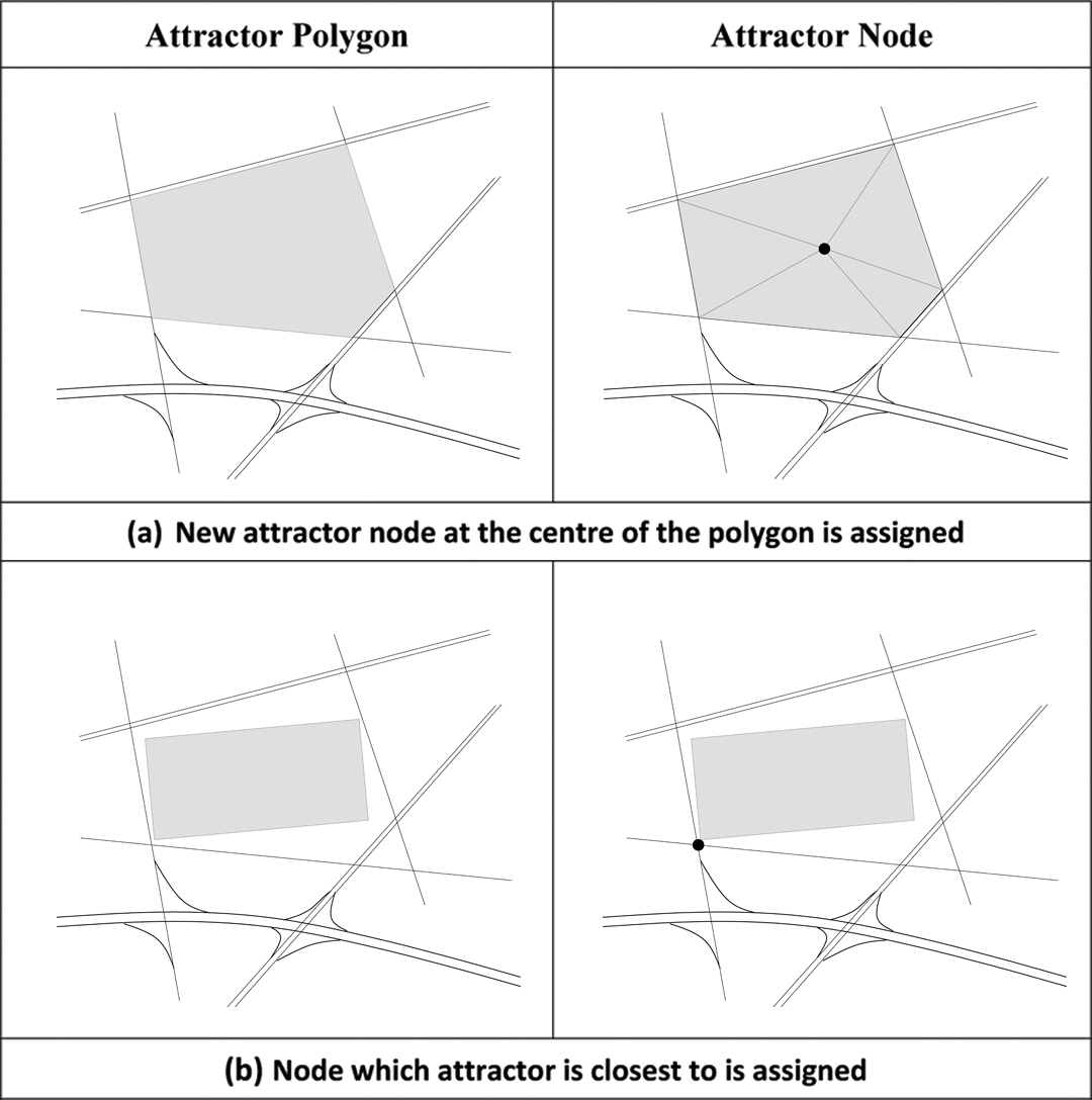
Defining nodes for attractors. A. New attractor node at the center of the polygon is assigned. B. Node which attractor is closest to is assigned.

The locations of offenders’ homes and the locations of the crimes they committed were also plotted on the road network. For these assignments, various forms of location identifiers were used. Specifically, offenders’ residences (identified by addresses) and locations documented as their corresponding crime sites (identified by an address, intersection, or street segment) were geocoded, recorded as coordinates, and finally plotted onto the road network. Because the simulated travel routes required start and destination points, the coordinates of home locations were snapped to the closest point on the network.

Assignment of Attractors

With the presence of multiple attractors in densely populated urban areas, it is necessary to assign the attractor that each offender would most likely choose to travel to on their journey to commit each crime. In order to do this, a variety of assignment rules were created. These rules were based on the offender’s home location and the locations of the crimes they committed. More specifically, the relation between the direction and distance characteristics of these features and the specified attractors were used in the assignment process.

The assignment process began with the measurement of the Euclidean distance between an offender’s home and each attractor. This resulted in five distance measures for each offender. Next, the Euclidean distance between each offender’s crimes and each attractor location was measured. This produced an additional five measurements for each crime attributed to an offender. Using these measurements, the assignment process included three conditional rules: (1) If the distance from an offender’s crime location to a particular attractor was less than the distance from the offender’s home to the same attractor, it was assumed that the offender was traveling in the general direction of that attractor. If that was the only attractor found to be in the direction of travel of that offender, it was assigned as that offender’s attractor location; (2) if, however, the crime location was in the general direction of multiple attractors, the attractor to which the crime location is nearest became the attractor assigned as the offender’s travel destination; and (3) if the direction from an offender’s home to crime location was not in the direction of any attractors, the attractor nearest the offender’s crime location was selected as his or her destination point.

By applying these assignment rules, it is assumed that each offender is traveling toward one attractor location. While assignments that fall under the third rule do not appear to be supported by the direction and distance characteristics of offenders’ crime locations, they were included in the current simulation to maintain a complete sample of property crime offenders. There is still a strong possibility that the closest major attractor was one that offenders traveled to, and thus would have contributed to the spatial patterning of their crimes. Figure 2 provides an example of the attractor assignment process. Two attractors, represented by black stars, are located in two geographically distant locations on the map. An offender’s home and crime location are also shown, represented by purple and green circles, respectively. Since the distance from the offender’s crime location to Attractor A is less than the distance between the offender’s home location and the other attractors, it is determined that the offender is traveling in the direction of Attractor A. As a result, Attractor A is selected as the offender’s destination point.

Figure 2.

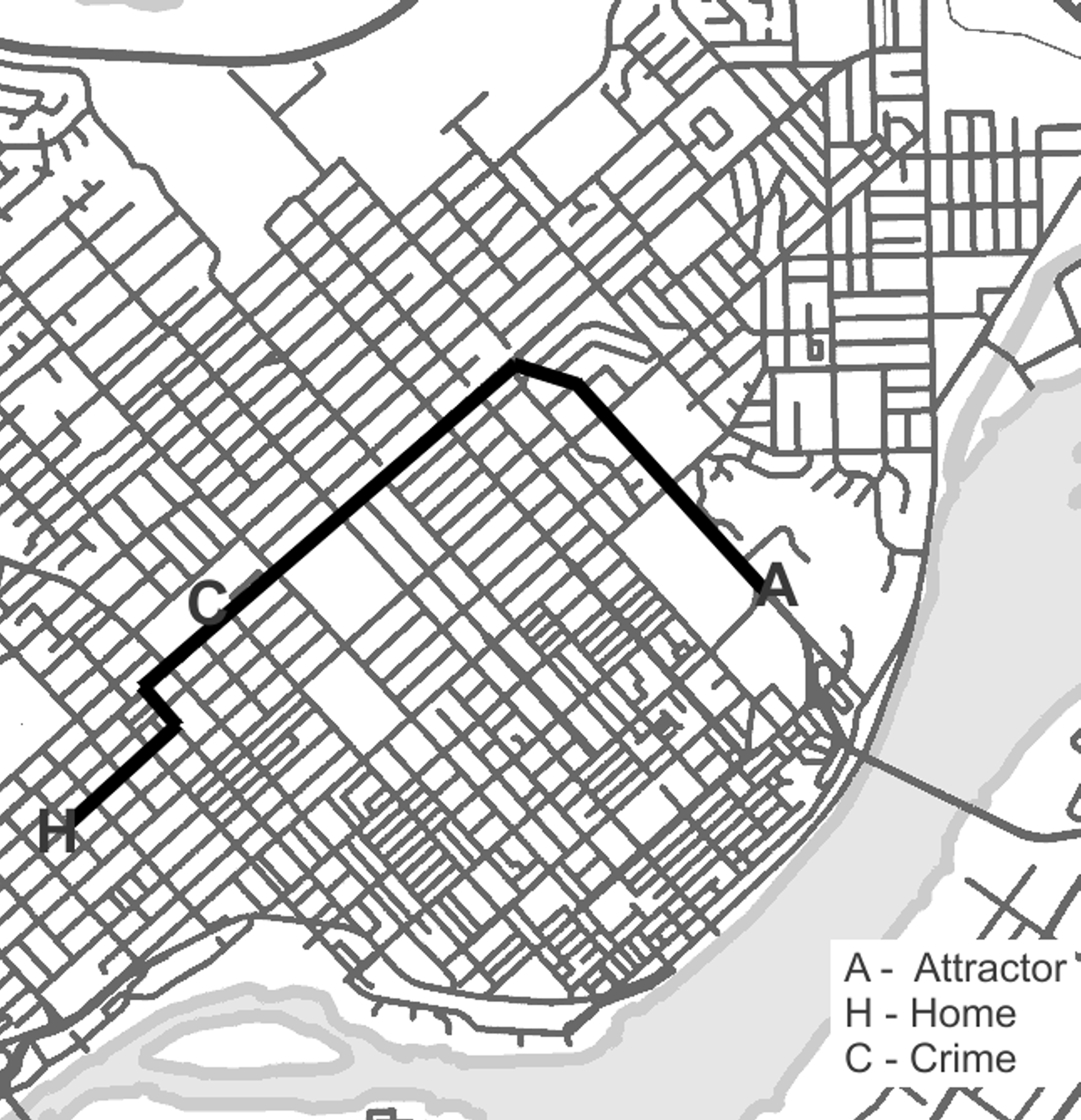
Assigning an attractor for an offender.

Generation of Travel Paths

With a place of origin and an assigned destination point, routes between an offender’s home and attractor may be generated. In order to effectively generate routes for large numbers of offenders, however, several assumptions are required. First, it was assumed that offenders most often travel along the road network. As a result, the simulated routes were restricted to movement along available road segments on the specified road network. In addition, it was assumed that offenders were interested in taking routes that were either the fastest in terms of time or shortest in terms of distance. Similar assumptions have been used in transportation studies because a path with the shortest distance may not necessarily be the fastest (Derekenaris et al. 2001; Devlin et al. 2008; Golledge and Stimson 1997). Furthermore, factors such as speed limit and the number of traffic control devices are likely to affect the appeal of a route to commuters. By using the shortest path and fastest travel time criteria for the selection of routes by offenders, Dijkstra’s algorithm (1959) was able to be applied.

Dijkstra’s algorithm generates the shortest and fastest travel routes between two locations. In our model, a random assignment, with each receiving a 50 percent probability, was given to all offenders determining whether the route will be one of shortest distance or fastest time. Once the algorithm calculated the appropriate type of route for each offender, the travel path was plotted on the road network.

Calculation of Distances between Crime Locations and Travel Paths

To evaluate the relationship between each offender’s crime location and the path from home to the attractor, several distance measures are calculated and analyzed, including Euclidean distance, Dijkstra distance, and Block distance. Euclidean distance provides the straight-line distance between the crime location and travel path, and makes no distinction about the specific location of the crime on the road network. Dijkstra distance provides a measure of the shortest distance or travel time along the road network between the crime location and the path generated between an offender’s home and assigned attractor. Because the calculation of Dijkstra distance requires measures between points and may not include partial distances between points, offenders’ crime locations were assigned to the nearest point on the network. Subsequently, Dijkstra’s algorithm was used to calculate the distance between the crime location and each point along the simulated travel path. The shortest of these distances was selected as the Dijkstra distance that can be used to represent the distance the offender detoured from their path in order to commit their crime. Finally, Block distance represents the number of city blocks required to travel from the simulated path to the crime site. This is calculated by counting the number of points or intersections that the offender would be required to travel through in order to arrive at the crime location after deviating off the simulated travel path.

Case Study—Greater Vancouver Regional District (GVRD)

Study Area

Three municipalities that are part of the GVRD, located in the southwest corner of British Columbia (BC), Canada, were selected as an amalgamated case study for the application of the model. Within these cities, five attractor locations were included as possible destinations for the offenders’ simulated trips. The layout of the municipalities is shown in Figure 3. Burnaby, Coquitlam, and Port Coquitlam are fast-growing urban cities that contain major commercial centers. Although they experience violent crime, property crime including motor vehicle theft is the category that accounts for the majority of crimes committed in these cities (BCStats 2010).

Figure 3.

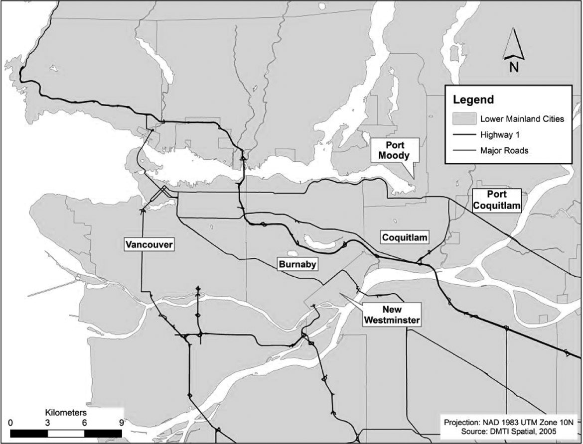
Map of Vancouver, Burnaby, and Coquitlam.

The City of Burnaby is adjacent to the east border of Vancouver. With a residential population of approximately 220,000, it is the third largest municipality in the GVRD (BCStats 2006). A major highway, Highway 1, divides the city into two—a distinct north and south area. Both of these areas are characterized by increasing commercial and industrial land use. The median family income of this city is $57,248 (Statistics Canada 2007a), which is less than the median family income of BC which stood at $62,346 in the 2006 census. It is home to many commercial, financial, and industrial firms. Metrotown, located in the southern region, is the city’s major commercial center and the largest shopping mall in the province. The area is surrounded by residential housing and has become a major crime attractor. Brentwood, Lougheed, and Highgate are three other major shopping centers in Burnaby and are also included as attractors in the model.

The City of Coquitlam is located directly east of Burnaby and has a population of approximately 125,000 (BCStats 2006). The median family income is highest in the province ($67,031 in 2006 (Statistics Canada 2007b). Although predominantly characterized by single-family dwellings and functioning primarily as a commuter town for the City of Vancouver, it has a growing commercial area—Coquitlam Town Centre. In addition to a major shopping mall, this area has a high-density residential area characterized by an increasing number of high-rise buildings that also includes the major transit station of the city with a direct train to downtown Vancouver. A library, city hall, a police station, and a college are also in its immediate surrounds.

The City of Port Coquitlam is a neighboring municipality of Coquitlam but has a much smaller residential population of approximately 50,000 (BCStats 2006). Located southeast of Coquitlam, it is a more isolated municipality with fewer attractors. Although it has commercial and industrial centers, Coquitlam Town Centre still functions as the major commercial zone in the area so it was included as the attractor for the latter two municipalities discussed.

Road Network

Road network data were obtained from GIS Innovations Ltd. for the year 2005. These data provide a particularly rich source of information regarding the streets and roads for the areas included in the model. In addition to the starting and ending coordinates of each road segment, the data provided detailed information about features such as the direction of travel along the segment, the length of the segment (in meters), the speed limit, and travel impactor information.

The road networks of five municipalities were included in the model. In addition to the three municipalities discussed above, Port Moody and New Westminster were included. Because the latter two municipalities are located near the northwest and southwest corners of Coquitlam, and many commuters pass through them when traveling throughout the region, it was important to allow for the opportunity of travel paths to be created in these areas. In total, 11,255 road segments constituted the road networks of these five municipalities.

Criminal Event and Offender Data

Crime data were obtained from two databases that contain five years of event and person information, respectively, for Royal Canadian Mounted Police jurisdictions throughout the province of British Columbia. Detailed information regarding calls for service between August 1, 2001, and August 1, 2006, is available in the data set. Subjects involved in a criminal event and their specific type of involvement are just some examples of the information that is available in the data set. For the current study, the two tables were linked to retrieve offender information for all criminal events.

Criminal event and offender data for individuals residing and committing crimes within Burnaby, Coquitlam, and Port Coquitlam were included in the current model. Ideally, other nearby municipalities would have been included in the current analysis to allow greater travel options in the region. Due to independent police forces holding contracts in Port Moody and New Westminster, comparable data were not available to be used in the current project. Offenders’ names, home locations, crime locations, and the types of crime committed were extracted and incorporated in the model. In total, 7,807 crime events were included.

In general, crimes may be categorized as those against a specific property (which are usually tied to a location) or those against a person (which are usually not tied to fixed locations) (Brantingham and Brantingham 1995). Because the current project emphasizes that location plays a central role, the application of the model is restricted to property crimes. Specifically, incidents of break and enter (burglary) and theft (including theft of and from a motor vehicle) were included in the current study.

Results

Figure 4 displays the aggregate paths taken from offenders’ home locations to one of the five possible attractor locations based on the attractor assignment rules and the simulated-path generation presented above. The color scale used to represent the paths shows heavily traveled routes identified in a dark color and less frequently traveled routes in a light color. Not surprisingly, routes near attractors and major arteries connecting the cities together are those most frequently traveled.

Figure 4.

Map of the paths taken by 7,807 offenders in the experimental evaluation.

By comparing these travel patterns and the locations of attractors with crime incidents in the region, interesting associations emerge. Figure 5 shows a kernel density map of property crime incidents for the five cities included in the model. The darkest shaded areas are the areas with the highest crime concentrations. The map shows a high degree of association between high-crime areas and the locations of crime attractors. This is an expected result because concentrations of crime are known to exist within the immediate surrounds of crime attractors (Block and Block 1995; Eck et al. 2007; Sherman, Gartin, and Buerger 1989). Of greater interest, however, is the association between high-crime areas and the routes leading to and from attractor locations. These routes are shown to be those most heavily traveled by offenders when they are traveling from their home location to an attractor. Given that the offenders travel these routes, their knowledge of the opportunities available will significantly increase, hence increasing their awareness space, and eventually the incidents of crime within those areas. Further, the majority of the paths taken by offenders fall into the major arteries within a city—those roads that also have greater concentrations of crime. This, too, is expected because criminal opportunities are known to have a greater likelihood of being exploited if they are on accessible and frequently traveled streets—this is particularly evident in the aggregate, because property crimes are most likely to occur on street segments that have high levels of traffic flow (Beavon, Brantingham, and Brantingham 1994).

Figure 5.

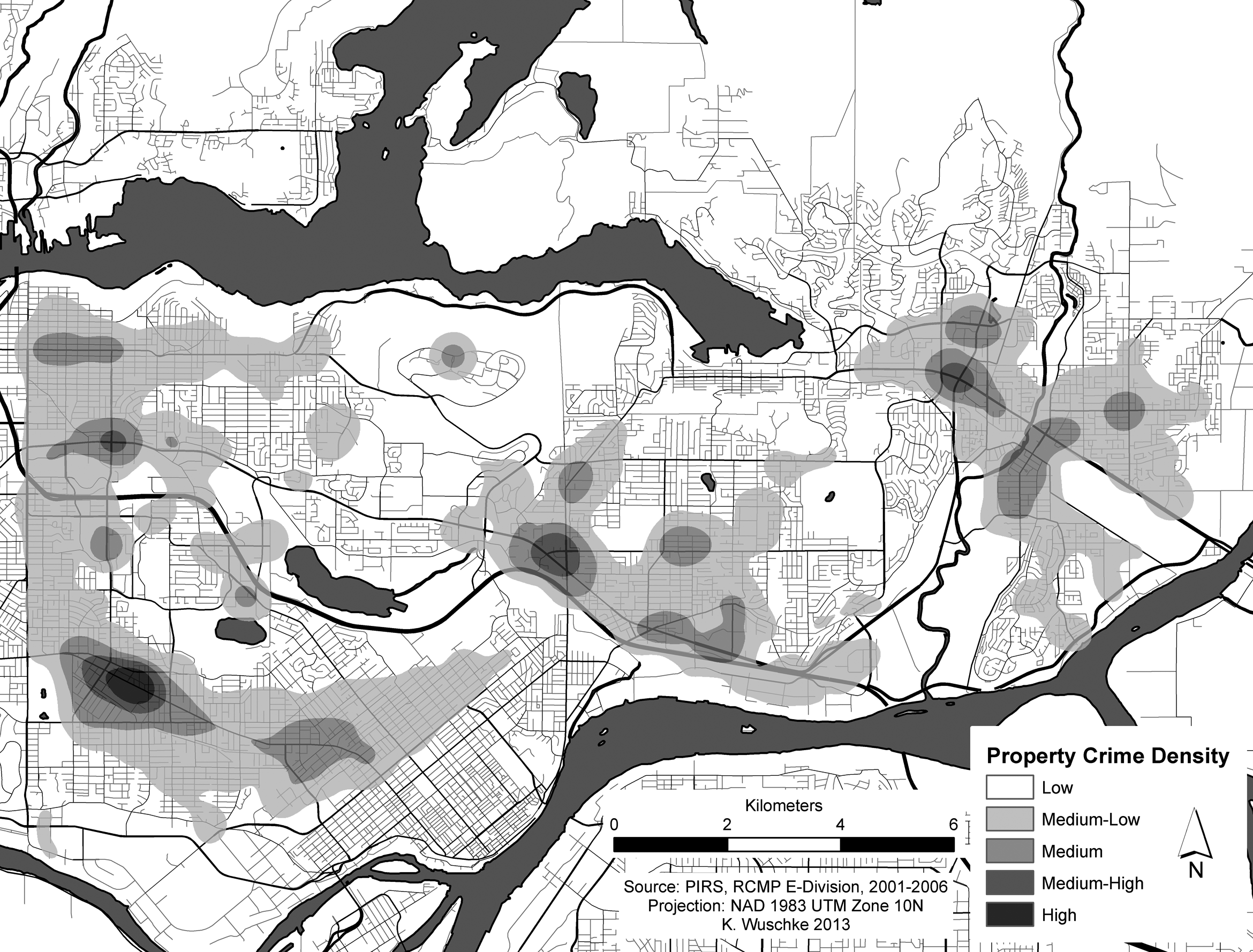
Kernel density map of property crime incidents within the Greater Vancouver Regional District between the years 2001 and 2006.

Figures 6 to 8 present results of the three distance measures that were calculated to show the relationships between travel paths of offenders and the actual crimes they committed. Results are presented using cumulative distribution functions to show the percentage of crime locations that were captured within a certain distance from each generated path. Figures 6, 7, and 8 present results for measures of Euclidean, Dijkstra, and Block distances, respectively.

Figure 6.

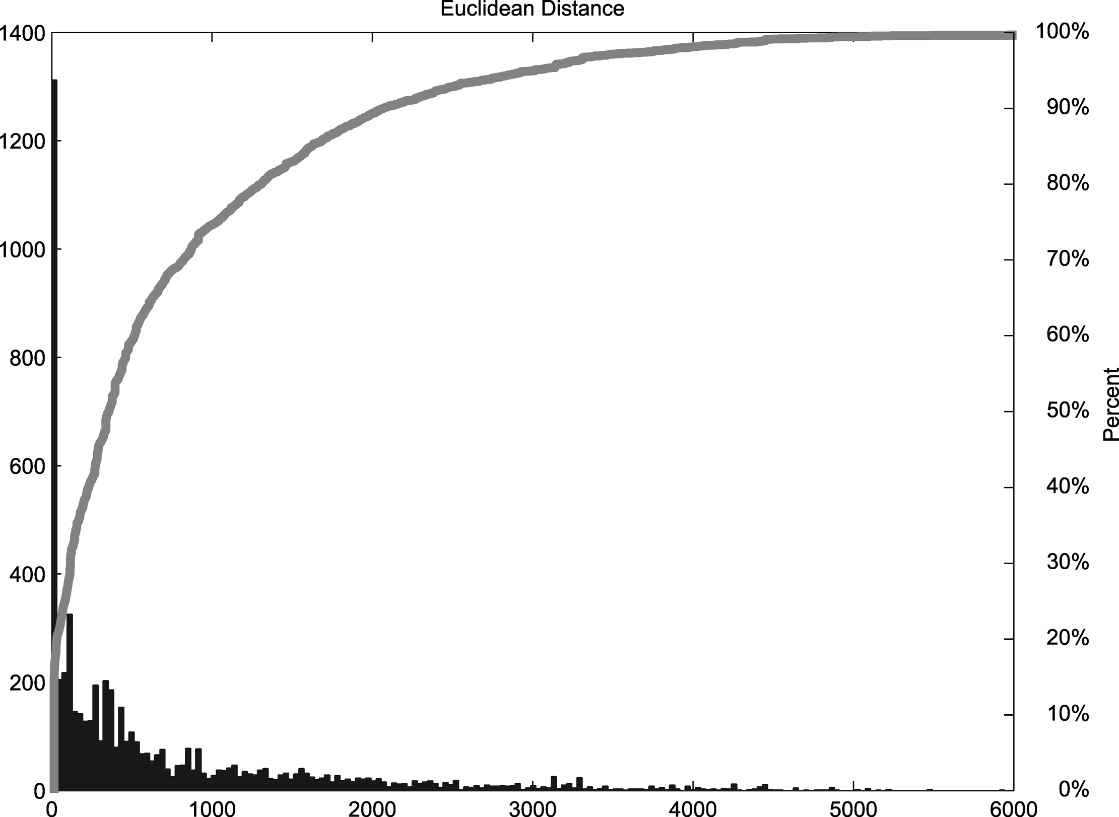
Cumulative Distribution Function plot of Euclidean distance between all crimes and paths.

Figure 7.

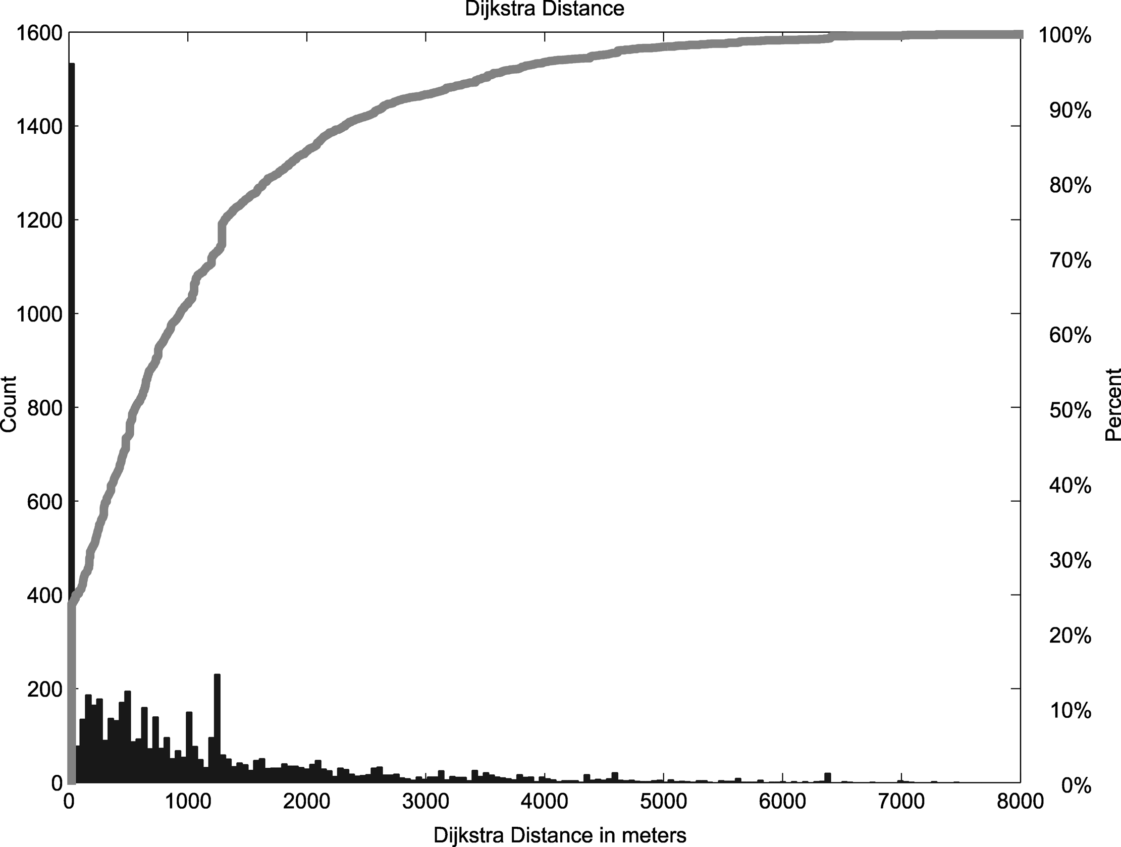
CDF plot of Dijkstra distance between all crimes and paths.

Figure 8.

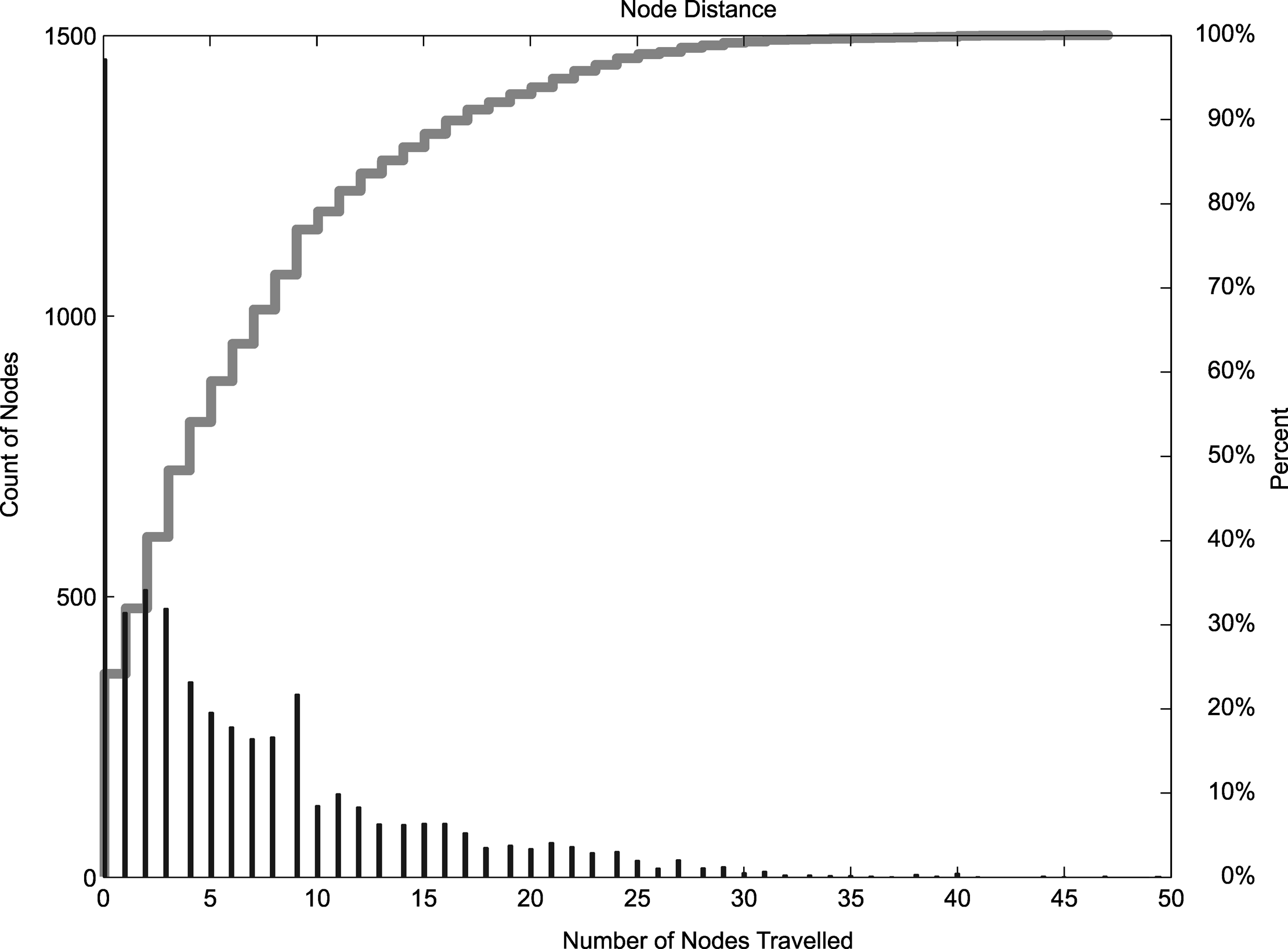
CDF plot of Block distance between all crimes and paths.

When considering Euclidean (straight line) distance, approximately 30 percent of all crimes are found to be within 32 m of the corresponding offender’s generated path; and 70 percent of all crimes are captured by a 500-m Euclidean distance (equivalent to a detour of a 5-min walk for the average person, or less than 1 min by car). Because there are fewer crimes located in the areas geographically distant from offenders’ travel paths, this pattern clearly shows a distance decay, starting from the path of the offender and extending outward. Thus, similar to Crime Pattern theory that argues for distance decay from activity nodes in the awareness spaces of offenders, paths between the nodes also exhibit the same distance decay pattern.

Euclidean distance measures, however, only begin to describe the relationships between travel paths and crime locations. Because offenders are most likely, and in the current model, assumed to be traveling along the road network, it is more accurate to describe distance measures that follow the road network. The cumulative distribution function for Dijkstra distance reveals a similar pattern to that of Euclidean distance. Approximately 35 percent of crime locations are located within 50 m of travel along the road network from the corresponding offender’s generated path. Approximately 70 percent of all crimes were located within 1,000 m when following the road network. As the distance between the crime locations and generated travel path increase, the amount of crimes in those distant areas decreases rapidly.

To provide a third interpretation of the distances between paths and crime locations, Block distance was calculated. The cumulative distribution function for Block distance reveals that 30 percent of all crimes were located zero points or city blocks away. The reason for these zero distance measures is that the crime locations were located along a road segment that was connected to the offender’s travel path. In effect, this means that the offender need not travel the full length of a single block distance or cross an intersection to arrive at the site where they committed the crime. Once again, a distance decay pattern is present whereby 68 percent of crimes were located within 5 blocks from their corresponding travel paths and fewer located further away.

Because the focus on this project is on areas traditionally considered crime neutral, it is important to ensure that crimes committed at attractor sites do not cause spurious results. This is particularly true for crimes such as shoplifting and motor vehicle theft which are likely to be concentrated at attractor sites such as shopping centers. To eliminate this as a possibility, the results were recalculated where all crimes located within 300 m of the five attractors were excluded from further analysis. This reduced the number of offenders included in the model to 6,055. Even with these offenders and their corresponding crimes removed, similar patterns are revealed: 30 percent and 70 percent of crimes were captured by 100 m and 800 m of Euclidean distance; 30 percent and 70 percent of crimes were captured by 150 m and 1,200 m of Dijkstra distance; and 24 percent and 70 percent of crimes were captured by zero and 8 Block distance.

Discussion

By mapping the most frequently traveled roads that emerged in the simulation that was carried out and comparing their locations to areas with elevated concentrations of crime, strong associations were discovered. Many of the most frequently traveled roads in the simulation were major arteries that lead to attractor locations and experienced elevated levels of crime. This is an expected result because in urban areas the routine activities of both criminals and noncriminals concentrate more people on certain roads, increasing the likelihood that the roads and some of the surrounding areas will be in their awareness space. This, in turn, is likely to result in offenders having knowledge about potential targets in these areas; therefore, it should be expected that property crimes will concentrate on or near major roadways. In a study conducted by Beavon et al. (1994), for example, a variety of street segment types were compared to explain variation in the amount of property crime. They found that opportunities for property crime have a greater chance at being acted on if they are on streets that are accessible and have increased traffic flow. Similar results have also been found in several other studies (see, e.g., Armitage 2007; Bernard-Butcher 1991; Johnson and Bowers 2010). Here, we see a similar pattern with the simulated travel routes that were plotted using Dijkstra’s algorithm.

We also found great proportions of offenders’ crimes located near the simulated travel paths. For all three distance measures—Euclidean, Dijkstra, and Block—approximately 70 percent of crimes were found to be within a 1-km or 5-Block distance from the offenders’ travel paths. Even more striking is that approximately 30 percent of all crimes were located a distance of around 50 m, or less than one block, from the associated travel path. These results suggest that, in many cases, offenders are not likely to take lengthy detours from their travel paths when committing crimes. They may, however, veer off their travel paths if a criminal opportunity is nearby.

These results provide strong support for Crime Pattern theory. A high percentage of crimes were found to be near the generated paths, indicating that offenders tend to commit crimes along paths leading to attractors and that these paths are part of their activity and awareness spaces. The results also highlight that an underlying pattern of crimes in crime neutral areas exists. Although the removal of crimes in the immediate surrounds of attractor locations clearly increased the distance measures required to capture the same proportions of offenders, similar proportions of crimes were still found to be located geographically proximal to offenders’ travel paths.

There are, however, some notable limitations to this work. First, only five attractor locations were selected to be included in the model. As a result, there may be additional attractors not accounted for that concentrate crimes along the routes to and from the attractors that were included. It should be noted, however, that many of the shopping malls used to represent attractors in this study also have other types of attractors in their immediate surrounds (e.g., rapid transit stations, large car parks, smaller commercial developments, and public buildings). By removing crimes located within a 300-m radius from each attractor and repeating the simulation, it is likely that much of this concern has been addressed.

A second limitation is that we assumed home locations of offenders to be the starting points of offenders’ travels. In reality, offenders could be traveling toward attractors from other places they frequently spend their time such as their legitimate place of work or school. Previous studies have shown that these other activity nodes play a significant role in offenders’ journeys to crime. For example, when analyzing the directional preferences of burglars, Rengert and Wasilchick (1985) found that a large proportion of burglaries were located near offenders’ workplaces and also along the routes between their home and work. Including these other possible starting points for offenders’ journeys to attractors could strengthen the results of our model and lead to further insights into the travel patterns of criminals. Such detailed information, however, is difficult to obtain for a large sample such as the one employed in the current study.

Third, the paths generated by Dijkstra’s algorithm may not mimic actual human travel patterns. In other words, the preferred routes of offenders may not necessarily be the shortest or fastest. Research has shown that there are many factors that impact the choices people make with respect to the routes they take (Liu 1996). People prefer to travel on major roads, they like to minimize the angle between their present location and their destination, and they typically choose familiar routes based on their previous driving experiences. Since Dijkstra’s algorithm does not take these factors into account, the routes generated in the model may differ from routes taken in real life.

Conclusion and Directions for Future Research

The Criminal Movement model (CriMM) presented in this article simulates travel patterns of offenders and compares them to the characteristics of the actual crimes they committed. The model selects a likely attractor location that serves as a destination point, simulates a shortest distance or fastest time route that an offender may take when traveling from their home to the attractor, and then compares the locations of the actual crimes the offender committed to the simulated travel path using three distance measures.

Results of the model showed that frequently traveled roads were often connecting arteries that led to attractor locations. These roads tended to correspond with locations that experienced elevated rates of crime. In addition, results of the three distance measures (Euclidean, Dijkstra, and Block) demonstrated that great proportions of crimes were located geographically near to the simulated travel path. These findings lend strong support to Crime Pattern theory and the idea that crimes, even those in crime neutral areas, are patterned.

In future developments of this project, we hope to extend the model by including more crime types and different study areas. Changing these two factors should allow us to confirm that the model is reliable and investigate how the geographical layouts of different cities affect travel patterns. CriMM could also be used to examine changes to the spatial arrangement of crimes when attractors are added or removed. By adding an attractor into the model, we should be able to predict the likely impact that the new activity node would have on the spatial patterning of crime in the surrounding area. It might also be possible to identify streets that would become more vulnerable to crime due to the increased number of people traveling along them.

Finally, in this article, attractor locations were assigned to offenders based on a specific set of rules that were derived from simple distance and direction measures. In future versions, we would like to extend CriMM into a predictive model where we can predict attractor locations based on the likely routes that offenders took to their crime locations. This would allow us to verify our assumptions regarding locations of attractors used in the current article and also discover new activity nodes that attract criminally motivated offenders.

Footnotes

Acknowledgments

The authors would like to thank Martin A. Andresen and the anonymous reviewers for their valuable comments and suggestions to improve the quality of the paper. The authors would like to thank Kathryn Wuschke for preparation of the map shown in .

Declaration of Conflicting Interests

The author(s) declared no potential conflicts of interest with respect to the research, authorship, and/or publication of this article.

Funding

The author(s) received no financial support for the research, authorship, and/or publication of this article.

Notes

References

Argent

N. M.

Walmsley

D. J.

. 2009. “From the Inside Looking Out and the Outside Looking in: Whatever Happened to Behavioural Geography’?” Geographical Research 47:192–203.

Armitage

2007. “Sustainability Versus Safety: Confusion, Conflict and Contradiction in Designing out Crime.” Pp. 81–110 in Imagination for Crime Prevention: Essays in Honour of Ken Pease (Crime Prevention Studies 21), edited by Farrell

Bowers

K. J.

Johnson

S. D.

Townsley

. Monsey, NY: Criminal Justice Press.

BCStats. 2006. “Census of Canada: Census Profiles.” Retrieved March 4, 2011(http://www.bcstats.gov.bc.ca/data/cen06/profiles/detailed/choose.asp).

BCStats. 2010. “Socioeconomic Profiles Regional Districts.” Retrieved March 4, 2011 (http://www.bcstats.gov.bc.ca/data/sep/rd/Rd_15.pdf).

Beavon

D. J. K.

Brantingham

P. L.

Brantingham

P. J.

. 1994. “The Influence of Street Networks on the Patterning of Property Offences.” Pp. 115–48 in Crime Prevention Studies, Vol. 2, edited by Clarke

. Monsey, NY: Criminal Justice Press.

Bernard-Butcher

(1991). “Crime in the Third Dimension: A Study of Burglary Patterns in a high-Density Residential Area.” Doctoral dissertation, Simon Fraser University, Burnaby, BC, Canada.

Bernasco

Luykx

. 2003. “Effects of Attractiveness, Opportunity and Accessibility to Burglars on Residential Burglary Rates of Urban Neighborhoods.” Criminology 41:981–1001.

Bernasco

Nieuwbeerta

. 2005. “How do Residential Burglars Select Target Areas? A New Approach to the Analysis of Criminal Location Choice.” British Journal of Criminology 44:296–315.

Liu

Bing

. 1996. “Intelligent Route Finding: Combining Knowledge, Cases and An Efficient Search Algorithm.” Pp. 380–84 in 12th European Conference on Artificial Intelligence (ECAI-96). Budapest, Hungary: John Wiley and Sons.

10.

Block

R. L.

Block

C. R.

. 1995. “Space, Place and Crime: Hot Spot Areas and Hot Places of Liquor-Related Crime.” Pp. 145–84 in Crime and Place: Crime Prevention Studies, Vol. 5, edited by In Eck

J. E.

Weisburd

. Monsey, NY: Criminal Justice Press.

11.

Brantingham

P. L.

Brantingham

P. J.

. 1981. “Notes on the Geometry of Crime.” Pp. 27–54 in Environmental Criminology, edited by Brantingham

P. J.

Brantingham

P. L.

. Beverly Hills, CA: Sage.

12.

Brantingham

P. L.

Brantingham

P. J.

. 1993. “Environment, Routine, and Situation: Toward A Pattern Theory of Crime.” In Routine Activity and Rational Choice: Advances in Criminological Theory, 5th ed., edited by Clarke

R.V.

Felson

. New Brunswick, NJ: Transaction.

13.

Brantingham

P. L.

Brantingham

P. J.

. 1995. “Criminality of Place: Crime Generators and Crime Attractors.” European Journal of Criminal Policy and Research 3:5–26.

14.

Brown

L. A.

Malecki

E. J.

Philliber

S. G.

. 1977. “Awareness Space Characteristics in a Migration Context.” Environment and Behavior 9:335–348.

15.

Derekenaris

Garofalakis

Makris

Prentzas

Sioutas

Tsakalidis

. 2001. “Integrating GIS, GPS, and GSM Technologies for the Effective Management of Ambulances.” Computers, Environment and Urban Systems 25:267–278.

16.

Devlin

McDonnell

Ward

. 2008. “Timber Haulage Routing in Ireland: An Analysis Using GIS and GPS.” Journal of Transport Geography 16:63–72.

17.

Dijkstra

E. W.

1959. “A Note on Two Problems in Connexion with Graphs.” Numerische Mathematik 1:269–271.

18.

Dreyfus

S. E.

1960. “An Appraisal of Some Shortest-Path Algorithms.” Operations Research 17:359–412.

19.

Eck

1993. “The Threat of Crime Displacement.” Criminal Justice Abstracts 25:527–46.

20.

Eck

J. E.

Clarke

R. V.

Guerette

R. T.

. 2007. “Risky Facilities: Crime Concentration in Homogeneous Sets of Establishments and Facilities.” Pp. 255–64 in Imagination for Crime Prevention: Essays in Honor of Ken Pease, edited by Farrell

Bowers

Johnson

Townsley

. Monsey, NY: Criminal Justice Press.

21.

Engelson

2003. “On Dynamics of Traffic Queues in a Road Network with Route Choice Based on Real Time Traffic Information.” Transportation Research Part C: Emerging Technologies 2:161–83.

22.

Frank

Andresen

M. A.

Brantingham

P. L.

. 2012a. “Criminal Directionality and the Structure of Urban Form.” Journal of Environmental Psychology 32:37–42.

23.

Frank

Andresen

M. A.

Brantingham

P. L.

. 2012b. “Visualizing the Directional Bias in Property Crime Incidents for Five Canadian Municipalities.” The Canadian Geographer/Le Géographe canadien 57:31–42.

24.

Golledge

R. G.

Neil

J. S.

Paul

B. B.

. 2001. “Behavioral Geography.” Pp. 1105–1111 in International Encyclopedia of the Social & Behavioral Sciences. Oxford, UK: Pergamon.

25.

Golledge

R. G.

Stimson

R. J.

. 1997. Spatial Behavior: A Geographic Perspective. New York: Guilford.

26.

Iwanski

Frank

Dabbaghian

Reid

Brantingham

2011. “Analyzing an Offender’s Journey to Crime: A Criminal Movement Model (CriMM).” Pp. 70-77 in Intelligence and Security Informatics Conference (EISIC), 2011 European. Athens, Greece: IEEE.

27.

Johnson

S. D.

Bowers

K. J.

. 2010. “Permeability and Burglary Risk: Are Cul-De-Sacs Safer?” J ournal of Quantitative Criminology 26:89–111.

28.

Kent

Leitner

Curtis

. 2006. “Evaluating the Usefulness of Functional Distance Measures When Calibrating Journey-To-Crime Distance Decay Functions.” Computers, Environment and Urban Systems 30:181–200.

29.

Lynch

1960. The Image of the City. Cambridge, MA: MIT Press.

30.

Rengert

G. F.

2004. “The Journey to Crime.” Pp. 169–81 in Punishment, Places and Perpetrators: Developments in Criminology and Criminal Justice Research, edited by Bruinsma

Elffers

Keijser

J. D.

. Cullompton, UK: Willan.

31.

Rengert

G. F.

Wasilchick

(1985). Suburban Burglary: A Time and a Place for Everything. Springfield, IL: CC Thomas.

32.

Rengert

George F.

Wasilchick

2000. Suburban Burglary: A Tale of Two Suburbs. Springfield, IL: C.C. Thomas.

33.

Sherman

L. W.

Gartin

P. R.

Buerger

M. E.

. 1989. “Hot Spots of Predatory Crime: Routine Activities and the Criminology of Place.” Criminology 27:27–56.

34.

Statistics Canada. 2007a. Burnaby, British Columbia (Code5915025) (table). 2006 Community Profiles. 2006 Census. Statistics Canada Catalogue no. 92-591-XWE. Ottawa. Released March 13, 2007. Retrieved from http://www12.statcan.ca/census-recensement/2006/dp-pd/prof/92-591/index.cfm?Lang=E. Accessed March 4, 2011.

35.

Statistics Canada (2007b). Coquitlam, British Columbia (Code5915034) (table). 2006 Community Profiles. 2006 Census. Statistics Canada Catalogue no. 92-591-XWE. Ottawa. Released March 13, 2007. Retrieved from http://www12.statcan.ca/census-recensement/2006/dp-pd/prof/92-591/index.cfm?Lang=E. Accessed March 4, 2011.

36.

Van Vliet

1978. “Improved Shortest Path Algorithms for Transport Networks.” Transportation Research 12:7–20.

37.

Wiles

Costello

. 2000. The Road to Nowhere: The Evidence for Traveling Criminals. U.K. Research study 207, Home Office, Research, Development and Statistics Directorate, London.

38.

Zhan

F.B.

Noon

C. E.

. 1998. “Shortest Path Algorithms for Transport Networks: An Evaluation Using Real Road Networks.” Transportation Science 32:65–73.