A Network of Neighborhoods

Abstract

Objectives:

Criminal target choice has been described as a multistage process: An offender first selects a suitable area from a set of alternatives and then chooses a specific target. This article studies area selection and attempts to distinguish between crime generators/visit detractors (elements that could affect anyone) and crime attractors/offense detractors (elements that affect offenders specifically).

Methods:

Trips that resulted in violent or property crimes between 506 census tracts in a large city (n = 11,411) are analyzed. Multilevel negative binomial regression is used to assess the impact of measures relating to pairs of tracts and characteristics of destination tracts.

Results:

Various factors are significantly related to the number of crime-associated trips per pair of tracts: differences in reward (residential and visiting population size, presence of schools or bars), differences in effort (distance between tracts, major roads linking both tracts), and differences in risk (level of social disorganization).

Conclusions:

This article supports an “opportunistic perspective” on crime: Crime-associated trips are more likely when advantages are high and risks and efforts are low.

Keywords

causes/correlates crime routine activity theory criminological theory social disorganization urban crime

One of the most frequent conclusions of researchers working on the geography of crime is that crime tends to be concentrated in particular spaces, and, naturally, they try to determine the characteristics that lead to such hot spots: for example, by identifying meaningful differences between high- and low-crime areas (e.g., Nelson, Bromley, and Thomas 2001; Wang and Arnold 2008). While many researchers on spatial criminology analyze the level of crime as an attribute of a particular area or place, others also discuss it in terms of relations between places and areas. Concepts such as nodes, paths, and direction are central to the study of journeys to crime, that is, journeys between an offender’s anchor point (e.g., home, workplace) and the place where she or he commits the infraction (Brantingham and Brantingham 1993; Frank, Andresen, and Brantingham 2012).

Rengert (2004) notes that three basic elements of a journey are of interest to criminologists: the starting point, the distance traveled by an offender from origin to destination, and the direction the offender moves in. The starting point has been the subject of many studies, which ask questions about where offenders live and what characteristics those communities have. As Bernasco and Block (2009) show, studies of the starting point of journeys to crime are primarily interested in understanding the motivation and “making” of offenders. A classic example is Shaw and McKay (1931), who observed, among other things, that neighborhoods characterized by high levels of crime also had high rates of population turnover, which made it difficult for communities to prevent criminality.

Another consequential set of studies of the journey to crime focuses on distance: The influence of distance is so apparent that some researchers prefer the term “distance to crime” to describe this aspect of their work (e.g., Andresen, Frank, and Felson 2014; Townsley and Sidebottom 2010) and distance has been an important aspect of analysis of spatial patterns (e.g., Rengert, Piquero, and Jones 1999; Van Koppen and De Keijser 1997). Consistent with many principles, including Zipf’s (1949) principle of least effort, the distance to crime is usually short (see Bichler, Christie-Merrall, and Sechrest 2011, for a review). This finding is one of the foundations of geographic profiling, a set of analytical techniques used to identify serial offenders (Rossmo 2000).

The present article looks at the third element of crime journeys—direction. Directional biases have been studied to investigate, among other things, what features of location and area attract motivated offenders (Rengert 2004). While there are a number of recent studies on where offenders choose to commit their offenses (e.g., Bernasco and Block 2009; Townsley et al. 2016), the literature dealing with why they pick these areas is limited, at least compared to the other two elements in crime journeys (Frank et al. 2012). In this article, we look at the factors that attract or discourage potential offenders from visiting specific census tracts (CTs) in a large Canadian city. The focus of analysis is on relations between tracts rather than the level of crime in these tracts.

Selecting a Suitable Area

Criminal target choice has been described as a multistaged process (Bernasco and Block 2009): From a set of alternatives, the offender first selects a suitable area and then chooses a specific target.¹ This analysis is supported by convincing empirical evidence: Crime in an area is not committed solely by residents but also by visitors (see Bernasco and Elffers 2010). While many authors have been interested in how specific targets are selected, often with crime prevention in mind (e.g., Clarke 1999), there are relatively few studies of the factors that explain area selection.

Three categories of predictors of offender location choice are generally distinguished: (1) differences in reward, (2) differences in effort, and (3) differences in risk (Townsley et al. 2016). Differences in rewards are measured by indicators of target availability and area affluence: For example, areas of commercial land use (especially areas containing shopping centres) in Burnaby, British Columbia, had considerably higher assault and motor vehicle theft rates than residential areas, suggesting a direct link between some activities and crime (Kinney et al. 2008). Stucky and Ottensmann (2009) found that violent crime was more likely in densely populated areas, supporting the idea that both offender and victim availability are important predictors of criminal opportunities. Other studies found that areas containing specific types of places were more attractive for specific types of crimes: For example, Bernasco and Block (2009) found that the presence of high schools and retail businesses make an area more attractive to thieves.

Differences in effort include various aspects of target vulnerability, such as characteristics of the urban “mosaic” (i.e., the presence of major roads) that facilitate the movement of offenders and thus increase the probability of crime (Bernasco and Block 2011; Stucky and Ottensmann 2009). Consistent with work on the distance to crime, there is consensus that the probability of an individual committing a crime in a particular area becomes less likely when distance increases: Areas located close to an offender’s home are more likely to be selected for crime, and crime-associated trips are more likely between nearby areas (Bernasco and Block 2009; Bernasco and Nieuwbeerta 2005; Elffers et al. 2008). Bernasco (2010) even found that offenders who commit robberies, residential burglaries, thefts from vehicles, and assaults are more likely to target areas in which they had formerly resided than similar areas they had never lived in, a finding he interprets as consistent with the concept of awareness space (Brantingham and Brantingham 1993). Offenders are more likely to be aware of criminal opportunities that occur within their awareness space, and this awareness varies depending on how long the offender lived in the area and whether she or he had moved away recently or some time ago (Bernasco 2010). Finally, the percentage of single-family dwellings, “which typically offer multiple street level entry-points [and] are likely both easier and less risky to physically access than flats, apartments, and attached dwellings” (Townsley et al. 2016:7; see also Bernasco and Nieuwbeerta 2005) has been found to be a significant factor.

Various indicators have been used to measure differences in risk between areas. Strong collective efficacy–social cohesion among neighbors combined with a willingness to intervene on behalf of the common good (Sampson, Raudenbush, and Earls 1997) has been found to reduce the probability that an area will be selected for crime (Bernasco and Block 2009). Indirect measures of formal and informal risk have also been investigated. Social barriers (i.e., racial and ethnic dissimilarity) influence the choices of some offenders but not others: For example, Black offenders are less likely to operate in a largely White neighborhood, presumably to avoid rapid detection (Bernasco and Block 2009; Bernasco and Nieuwbeerta 2005; Stucky and Ottensmann 2009). Areas known to contain illegal markets have been found to be particularly attractive to thieves; in contrast, gang territories are avoided by some (e.g., members of rival gangs) but may be attractive to others (Bernasco and Block 2009, 2011).

Social Network Analysis in Spatial Criminology

Crime pattern theory (Brantingham and Brantingham 1993, 2008) understands crime as a complex phenomenon that has some consistent aspects, a perspective that has been useful in the study of the geography of crime. For example, Weisburd, Groff, and Yang (2012) found that hot and cold spots of crime in the city of Seattle remained largely stable over a period of 16 years. In other words, not only did they find concentrations but their results also suggest that a set of common factors might be associated with crime levels. Following routine activities theory, crime pattern theory further argues that “[w]hat shapes non-criminal activities helps shape criminal activities” (Brantingham and Brantingham 2008:79). Crime pattern theory involves the existence of an “urban backcloth”—the spatial structure that results from community planning and development—that shapes individual behaviors and ultimately creates the context that allows crime to occur when criminal opportunities arise (see also Bichler, Malm, and Christie-Merrall 2011).

The description of such a “grid” appeals to social network analysts who have studied the interlocking relations of social life since the 1930s (Scott 2013). A journey to crime establishes a relationship between two places or areas and the accumulation of these relationships forms a network of places or areas. In addition to studies of journey to crime, we were able to locate three recent studies published in leading journals that use formal Social Network Analysis techniques to test a concept related to the geography of crime, the analysis of relations between areas. The first study (Schaefer 2012) investigated the presence of ties between neighborhoods based on co-offending by youth—two CTs were seen as linked if a youth from tract i committed an infraction with a youth from tract j. Schaefer’s argument, an extension of theories of social learning and differential association (e.g., Sutherland 1947), is that crosstract offending can increase the diffusion of information, skills, norms, and behaviors across neighborhoods. His analysis provides various insights: (1) he found a high degree of spatial clustering of co-offending, indicating the importance of geographic distance; (2) controlling for spatial proximity, social distance indicators showed that large differences between tracts decreased tie likelihood; and (3) several measures of tract characteristics (percentage of youth aged 10–17 years, one-parent households, residential instability, and juvenile criminal activity) increased the likelihood, supporting the expected relationship between social disadvantage (also known as social disorganization) and crime. While these findings could be expected, given the large empirical literature in this area, Schaeffer provides evidence that most of the factors identified were not only linked to an increase in the level of crime in an area but could also explain the structure of co-offending networks at neighborhood level.

The second study (Bichler, Malm, and Enriquez 2014) focused on identifying “magnetic places” where delinquent youth converge. The argument is that crime prevention requires information about the places frequented by youths during their discretionary time (see also Felson 2003). Data on the travel behavior of youths at 144 schools in California were used to create networks of places identified as activity nodes. In-degree and betweenness centrality were used to assess the temporal stability of key places in the region. Bichler et al. found that shopping complexes, especially when situated nearby large movie theaters, consistently attracted youths from different schools. More importantly, the Bichler et al. study draws upon the Brantingham and Brantingham (1993) classification of places, arguing that “magnetic places” are crime generators in that they attract many people, including some who will commit opportunistic crimes: Crimes are more frequent in neighborhoods that attract large numbers of visitors, and crime-related trips should be more frequent toward an area that attracts many people. They noted that this relation is as “trivial” as the one between population and crime: the larger the population of an area, the larger the number of crimes committed in that area—a function of availability of likely offenders and suitable targets. Brantingham and Brantingham (1993) also found that areas that are crime attractors have characteristics that are particularly attractive to highly motivated offenders. They may, for instance, be “underpoliced” or provide criminal opportunities and places where individuals with histories of repeat offending can meet. Finally, they identified crime-neutral areas, that is, “areas that neither attract intending offenders because they expect to do a particular crime in the area, nor do they produce crimes by creating criminal opportunities that are too tempting to resist” (Brantingham and Brantingham 2008:89). Characteristics associated with these processes are defined as crime detractors: Visit detractors discourage people’s presence or indicate places and areas that contain few attractions whereas offense detractors refer to places that are specifically avoided by likely offenders. In both cases, journeys to such areas are expected to be less frequent.

The most recent study, by Davies and Johnson (2015), looked at the risk of burglary as related to the configuration of street networks in Birmingham (United Kingdom). They found that the number of burglaries on a given street segment was strongly related to betweenness centrality and interpreted this result as evidence that more frequently used segments are at higher risk for such crime. Their findings strongly support the routine activities theory (Cohen and Felson 1979), which argues that crime is often opportunistic and dependent on the convergence of a likely offender and a suitable target in the absence of capable guardianship. Perhaps more relevant to the current study, Davies and Johnson show that network measures can be used to predict the level of crime in an area, providing support for the idea that directionality (the direction and paths people use to move from one activity node to another) is of special interest to those analyzing crime (see also Frank et al. 2012).

Current Study

Previous researchers have found that significant increases or decreases in criminal activity are associated with various factors and have hypothesized about the sort of individual who might be attracted or detracted by such factors. However, they have not been able to empirically separate crime generators/visit detractors (factors that could affect anyone) from crime attractors/offense detractors (factors that appeal largely to offenders). Being able to make this distinction has crucial implications for law enforcement agencies and crime prevention organizations.

In this article, we investigate various characteristics of specific areas that attract or deter visitors and offenders. Adapting the typology of places created by Brantingham and Brantingham (1993) to describe larger areas such as tracts and neighborhoods, we contribute to the literature by using data from a large transportation survey to control for noncrime-associated trips, which makes it possible to separate out crime generators and attractors as well as visit and offense detractors (see Figure 1).

Figure 1.

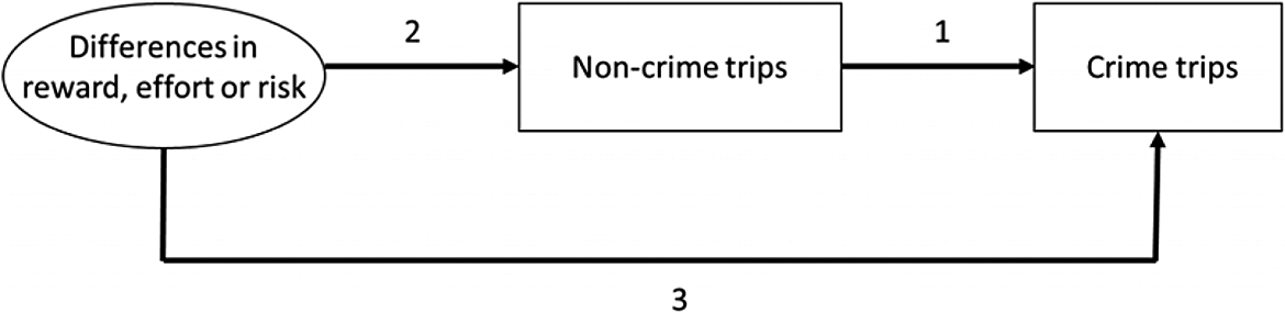
Possible relations between predictors, noncrime-associated trips, and crime-related trips.

Differences in reward, effort, and risk can be assumed to be crime generators if they are associated with an increase in the number of noncrime-associated trips between two tracts (arrow 2) and if the number of noncrime-associated trips is a positive predictor of the number of crime-associated trips (arrow 1); a factor only considered a crime generator should not be a significant predictor of crime-associated trips (arrow 3). Some characteristics may be especially attractive to potential offenders: when noncrime-associated trips can be controlled for, a characteristic is a crime attractor, as opposed to a crime generator, if it significantly increases the number of crime-associated trips between two tracts (arrow 3), whether or not it is significantly related to noncrime-associated trips (arrow 2). In contrast, some areas might involve factors—crime detractors—that are avoided by visitors and/or likely offenders and thus decrease the number of trips (crime-associated trips or not) between two tracts. This strategy is similar to the one put forward by Elffers et al. (2008), who studied spatial flows between 94 neighborhoods in the city of The Hague (the Netherlands) using geographical distance and “intervening opportunities” as predictors and conclude that geographical distance is the main predictor of crime trips between two areas, supporting the importance of considering relational characteristics even at neighborhood level.

Methods

Police-recorded statistics from 2013 at CT level for a large city in eastern Canada were used. The Police Department provided the geolocation of crimes at CT level. The analysis includes only cases for which the home address of the main offender was available, which occurred when cases were cleared by charge or cleared otherwise.² Only crimes committed by nonresidents—crimes committed in a tract different than the offender’s home tract—were analyzed because it was assumed that they involved a trip by the offender. Cases involving multiple main offenders were not provided to the researchers to avoid inconsistencies. A total of 11,411 crime trips were analyzed. Two specific categories of crime were analyzed: violent (n = 5,451) and property (n = 5,960). Statistics Canada’s definitions were used (see Boyce 2015, for details): violent crimes include, among others, homicide, sexual and nonsexual assault, robbery, and kidnapping, while property crimes include breaking and entering, various forms of theft, and fraud.

Noncrime trips were measured using a 2011 transportation survey of 66,100 households (approximately 156,000 individuals) that included questions about locations where respondents work and shop or engage in recreation and education. The total of 1,816,180 trips allowed us to estimate daily population flows between each CT.

The unit of analysis was relations between CTs as measured by the number of trips from tract A to tract B. The result was matrices (i.e., directed value networks) of trips between 520 CTs, for a total of 269,880 dyads (520 × 519). Networks were built for five outcomes: noncrime-associated trips and trips involving violent crime, property crime, crimes committed by adults, and crimes committed by youths.

Independent Variables

The goal of this article is to understand what attracts or discourages likely offenders from committing crime in certain areas. Since the outcome is relational (number of trips between two tracts), the next section describes various indicators that were used to measure characteristics of (1) the relation and (2) the destination (the head end). These characteristics were selected on the basis of existing empirical evidence and data availability.

While the number of characteristics of the relation is limited, three characteristics are essential to our understanding of crime-associated trips as conceived by Brantingham and Brantingham. The first is distance: As gravity models of macroscopic relations between places posit, the number of crime-associated trips should decrease with increasing distance (Anderson and van Wincoop 2004; Tinbergen 1962). Centroid distance between tracts in meters is used in the analysis. The second relational predictor in the analysis is another measure of effort: the presence of at least one major road (highway or boulevard) between both tracts (0 = no major road; 1 = at least one major road). The third characteristic is actually one of the outcomes: the number of noncrime-associated trips. As mentioned previously, crime generators are factors that attract all kinds of people, thus generating opportunities for crime. In order to be able to identify the effect of other predictors, one needs to control for the “generator” effect. In the vocabulary of statistical modeling, noncrime-associated trips are expected to have moderating effects on the relationships found between various predictors and crime-associated trips.

Some areas (e.g., downtown areas) are attractive to a variety of people for various reasons. The total number of visits—regardless of origin—to a CT, estimated through the transportation survey, was included as a measure of the overall popularity of the area.³ The number of two types of establishments in the area (identified from the literature)—licensed premises serving alcohol (bars, pubs) and schools—was also included and was extracted from a list of businesses and industries in the city.

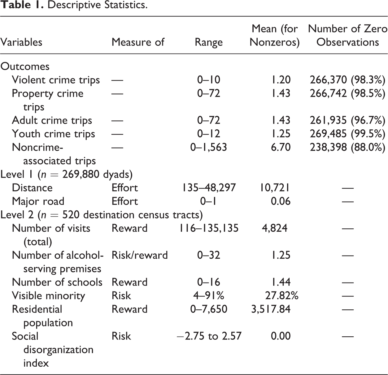
Other characteristics were taken from the 2011 Canadian Census.⁴ The characteristics of the residential population are often used as indicators of the number of potential targets in an area. The proportion of visible minority persons, as defined by the government of Canada, has often been used in studies of crime in the United States and is used as one indicator of the level of social disorganization in an area (Bruinsma et al. 2013); however, in the city under study, the proportion of visible minority individuals is not highly correlated with other measures of disadvantage (see Appendix Table A1), so we excluded it from the social disorganization index but included it in the models because it appeared in all previous studies of offender location choice. The social disorganization index includes three highly correlated measures: five-year residential mobility, proportion of single-parent families, and proportion of low-income households in the tract. Table 1 presents descriptive statistics for dependent and independent variables.

Table 1.

Descriptive Statistics.

Variables	Measure of	Range	Mean (for Nonzeros)	Number of Zero Observations
Outcomes
Violent crime trips	—	0–10	1.20	266,370 (98.3%)
Property crime trips	—	0–72	1.43	266,742 (98.5%)
Adult crime trips	—	0–72	1.43	261,935 (96.7%)
Youth crime trips	—	0–12	1.25	269,485 (99.5%)
Noncrime- associated trips	—	0–1,563	6.70	238,398 (88.0%)
Level 1 (n = 269,880 dyads)
Distance	Effort	135–48,297	10,721	—
Major road	Effort	0–1	0.06	—
Level 2 (n = 520 destination census tracts)
Number of visits (total)	Reward	116–135,135	4,824	—
Number of alcohol- serving premises	Risk/reward	0–32	1.25	—
Number of schools	Reward	0–16	1.44	—
Visible minority	Risk	4–91%	27.82%	—
Residential population	Reward	0–7,650	3,517.84	—
Social disorganization index	Risk	−2.75 to 2.57	0.00	—

Analytical Strategy

Traditional regression modeling cannot be used for this analysis, for two main reasons. First, outcomes are relational, with the consequence that single tracts are involved in multiple dyads. Models of network regression (Quadratic Assignment Procedure [QAP], Exponential Random Graph Models [ERGM]) have been developed over the years to account for this issue of dependence between observations but are of limited use here because they tend to concentrate on the presence/absence of a relation between two units (Wilson et al. 2017). A different strategy is used here: Mixed (multilevel) models using crossed random effects are used to control for potential errors due to the clustering of units into dyads. Level 1 accounts for dyads (n = 269,880) and level 2 for destination CTs (n = 520).

These strategies are useful for relational data but do not necessarily account for a second potential issue: It was suspected that dependent variables, as mentioned above, were distributed in a way that fits the definition of overdispersed count variables (for a more complete discussion, see Land, McCall, and Nagin 1996).⁵ The average number of trips per dyad is well under 1, with the exception of noncrime-associated trips. Furthermore, excessive 0 values are evident (see Table 1). To account for these highly skewed distributions, two statistical models were tested for each outcome: a regular negative binomial regression model and a zero-inflated negative binomial regression model that aims to correct for excessive zeroes. The main difference between both strategies is that zero-inflated regression generates two separate models, whereas regular negative binomial regression provides only one. Both techniques yield count models that predict a given discrete value, but zero-inflated regression separates zero and nonzero-values by modeling (1) a logit “inflate” model for predictions of excess zero values (the probability of no trips vs. at least one trip between two tracts) and (2) a count model for nonzero values (the number of trips between two related tracts for all nonzero valued dyads). Some find that the logit model is counterintuitive, as it predicts an absence (0 value = 1) versus a presence (value of 1 or more = 0). However, a negative relation in the inflate model followed by a positive relation in the count model are perfectly consistent and vice versa. In the following, only the best performing models are presented, that is, the model with the lowest Bayesian information criterion: zero-inflated for noncrime-associated trips, regular for all four types of crime-associated trips. Mplus Version 7.4 was used for multivariate analysis and SPSS Version 23 was used for univariate and bivariate analyses.

Results

Predictors of Noncrime-associated Trips

Table 2 presents zero-inflated negative binomial models in two parts: an inflate model predicting the probability of zero trip (binary outcome/logit model) and a negative binomial model predicting the number of trips (count outcome, values of 1 or more).

Table 2.

Zero-inflated Negative Binomial Regression Models for Noncrime Trips.

Variables	Noncrime-associated Trips (Inflate Model)	Noncrime-associated Trips (Count Model)
Level 1 (dyads)
Distance	.523**	−.905**
Major road	−.117**	.290**
Level 2 (destination census tract)
Number of visits (total)	−.990**	.490**
Bars	.015	−.015
Schools	−.032	.113**
Visible minority	.002	−.065
Residential population	−.095**	.223**
Social disorganization index	.047	−.362**
Variance (level 1)	.402
Variance (level 2)	.036
Intraclass correlation coefficient	.082

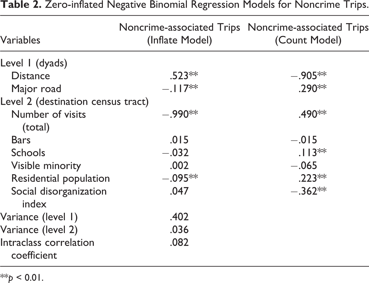
**p < 0.01.

As expected, distance is a significant predictor of the number and probability of noncrime-associated trips. This confirms the existence of a distance decay for visits; distant tracts are less likely to be visited and the number of visits decreases with distance. However, the presence of a major road increases visits between two tracts. Both variables show stronger relationships with the number of trips (count model) than with the likelihood of at least one trip (inflate model) as shown by the absolute value of the β coefficients presented in Table 2. This is due in part to the fact that major roads are more likely between nearby areas; both variables are dimensions of the concept of geographic proximity and both statistical relations are consistent. These results are not only consistent with the idea that differences in effort explain (crime) trips, but also that major roads act as physical connectors that facilitate access and reduce the impact of distance (Clare, Fernandez, and Morgan 2009; Johnson and Summers 2015).

Controlling for geographic proximity, popular areas—as measured by the total number of visits—is more likely to be destinations. The presence of schools and residential population size also increases the number of noncrime-associated trips to a given area. On the contrary, indicators of economic and social deprivation decrease the number of trips toward an area. As shown by the intraclass correlation coefficient, most (91.8 percent) of the variance is explained by relational variables (level 1), rather than characteristics of destinations, again supporting the importance of geographic proximity.

Displacements with Criminal Outcome

The main objective of this article was to investigate whether factors (such as size of population and presence of various establishments) affected everyone or if they specifically attracted or repelled potential offenders. Table 3 shows negative binomial regression models containing the same set of predictors but controlling for noncrime-associated trips. Significant relations indicate that these factors are particularly prominent for potential offenders.

Table 3.

Negative Binomial Regression Models for Crime Trips.

Variables	Property Crime	Violent Crime	By Youths	By Adults
Level 1 (dyads)
Distance	−0.936**	−0.941**	−0.817**	−0.930**
Major road	0.121**	0.095**	0.150**	0.120**
Noncrime trips	0.131**	0.143**	0.368**	0.150**
Level 2 (destination census tract)
Number of visits (total)	0.356**	0.101	0.176**	0.266**
Bars	−0.018	0.175**	0.085	0.153**
Schools	−0.224**	0.060	0.226**	−0.048
Visible minority	−0.058	−0.052	−0.155**	0.003
Residential population size	0.368**	0.415**	0.254**	0.375**
Social disorganization index	0.143**	0.184**	0.038	0.200**
Variance (level 1)	14.114	12.963	140.464	3.918
Variance (level 2)	1.43	0.548	1.316	0.505
Intraclass correlation coefficient	0.092	0.041	0.009	0.114

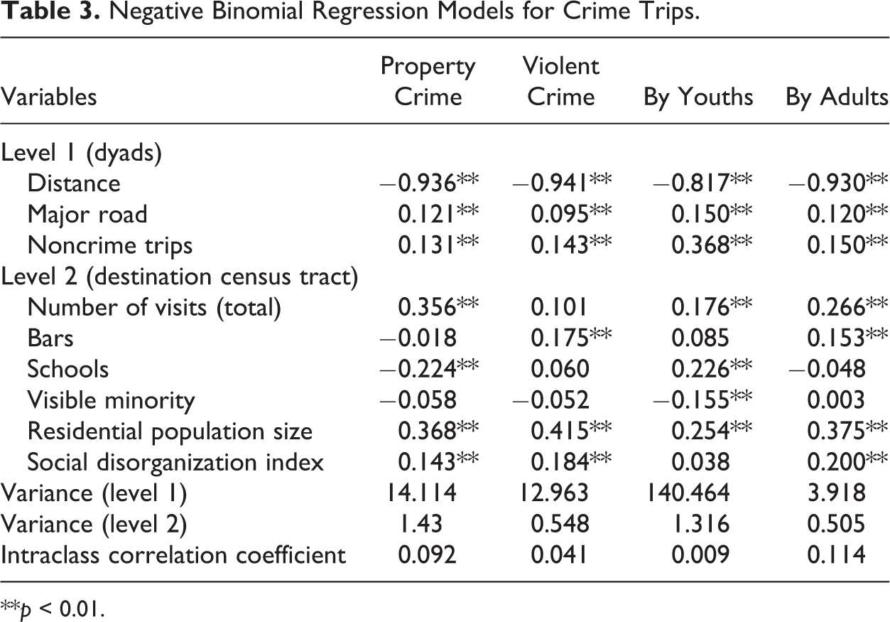
**p < 0.01.

The number of noncrime-associated trips between two tracts is, unsurprisingly, a significant positive predictor of the number of crime-associated trips. This was expected because an abundant literature describes the opportunistic nature of many crime incidents. Distance and the presence of a major road are again significant predictors, suggesting that differences in effort are especially important in understanding crime-associated trips.

Two measures of differences in reward (residential population size and number of visits) are positively and significantly related to the number of crime-associated trips, showing that affluent areas are preferred by potential offenders. However, the total number of visits is unrelated to trips associated with violent crime. The fact that the number of licensed establishments in an area is positively associated with trips associated with violent crime (but not with trips associated with property crime) supports the observation that violent crime is often the result of the convergence of assailants and victims in a context perceived as permissive. Bars are known to be places where the risk of being a victim of assault is high compared to other commercial settings (Burrows et al. 2001). Alcohol lowers inhibitions and potential offenders tend to misbehave, especially if they perceive low risk of punishment (Graham et al. 2006; Pihl and Peterson 1993). Managing aggression in bars has long been identified as a challenge and risks of apprehension are lower in bars, especially if the two parties are “consensually” involved in the incident (e.g., a fight; Graham 2009; Graham, Jelley, and Purcell 2005).

Other measures of risk are inconsistently related to the outcome. The proportion of visible minorities among residents is negatively related to crime-associated trips, but only for youths. Perhaps more interestingly, social disorganization is positively related to all outcomes except crimes by youths, a result consistent with the existing literature that shows that disorganized communities are not able to control criminal activity in their territory.

Table 3 also supports two general conclusions. The first is that different outcomes require different explanations at tract level. Predictors of property crime are not the same as those for violent crime nor is the strength of relations—the same can be said about crimes committed by youths and by adults. The second is that characteristics of destination tracts explain at best 11.4 percent of the variance, meaning that the most important predictors of crime-associated trips in our models are differences in effort and that crime-associated trips are better understood based on relational predictors.

Crime Generators, Attractors, and Detractors

In their formulation of crime pattern theory, Brantingham and Brantingham (1993, 2008) proposed a typology of places that also has been applied to predictors of trips between CTs (see Table 4). The analysis presented above shows evidence of crime detractors, that is, factors that deter people from visiting, thus decreasing the number of trips. Distance is the strongest predictor in all models, thus confirming the abundant literature on distance decay that finds that human activity is less likely as one moves further from the starting point. Furthermore, controlling for distance, the presence of a major road linking two tracts is significantly and positively related to all count outcomes, which strongly supports the idea that offenders target tracts more accessible via the street network, a result similar to Johnson and Summers (2015). As argued by Brantingham and Brantingham (2008), the configuration of the street network dictates our routine, and potential offenders should be more likely to be aware of criminal opportunities in places that are easily accessible. Supporting this proposition is the fact that a measure of differences in reward (number of visits and residential population size) was also found to be both an attractor and a generator. In other words, both factors that explain the popularity of a destination are associated with an increase in crime counts, thus suggesting that crime prevention measures in these dyads should apply to the population as a whole because, while motivations to visit may differ, crime is likely to be the result of increased opportunities.

Table 4.

Summary of Results (Count Models Only).

Variables	Measure of	Relation with Noncrime- associated Trips	Relation with Crime- associated Trips	Type
Level 1 (dyads)
Distance	Effort	−	−	Detractor
Major road	Effort	+	+	Attractor/generator
Level 2 (destination census tract)
Number of visits (total)	Reward	+	+/n.s.	Attractor/generator
Bars	Risk/reward	n.s.	+/n.s.	Attractor
Schools	Reward	+	±/n.s.	Mixed
Visible minority	Risk	n.s.	−/n.s.	Offense detractor
Residential population size	Reward	+	+	Attractor/generator
Social disorganization index	Risk	−	+/n.s.	Mixed

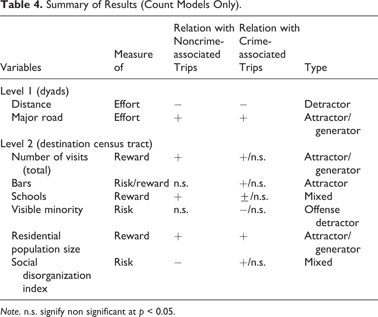
Note. n.s. signify non significant at p < 0.05.

Other factors show mixed relationships with outcomes. First, schools were found (as expected) to increase the number of trips but decrease the number of trips involving property crime, perhaps because students and parents may act as guardians or because students are not interesting targets. However, schools increase crime-associated trips by youths, suggesting that youths commit opportunistic crime close to the place where they spend most of their time. Second, the number of bars in the destination tract increases trips associated with violent crimes and adult offenders. Bars have already been identified as crime attractors for various reasons (Britt et al. 2005; Gruenewald et al. 2006; Livingston 2008), but the analysis emphasizes the idea that their presence attracts likely offenders more than “ordinary” people. Third, social disorganization was found to be negatively related to noncrime-associated trips but positively related to crime-associated trips—it appears to push visitors away but pull in offenders. These results nuance previous research that suggested that social cohesion (i.e., often presented as the opposite of social disorganization) may act as a deterrent when offenders target an area (Bernasco and Block 2009; Bernasco and Nieuwbeerta 2005; Clare et al. 2009; Johnson and Summers 2015). While the analysis presented in the current article offers partial support for this hypothesis—social disorganization is significantly associated with a reduced number of noncrime trips—the opposite is found for criminal trips: Social disorganization is associated with an increased number of criminal trips. Social disorganization appears to act simultaneously as a visit detractor and a crime attractor, showing the importance of distinguishing factors that could affect anyone from factors that appeal specifically to offenders.

Limitations and Conclusion

Much of the evidence presented in this article supports an “opportunistic perspective” on crime: Crime-associated trips are more likely when rewards are high and risks and efforts are low. The analysis also supports the Brantingham and Brantingham (2008) argument that a better conceptualization of the urban backcloth can help in understanding offenders’ travel patterns. However, there are reasons to believe that the analysis underestimates “purposeful” crime trips because of limitations inherent to the data set used. In particular, intratracts trips (i.e., by residents) were excluded. These are likely to be numerous because individuals are more aware of opportunities in their immediate environment—a phenomena that Brantingham and Brantingham (1993) touch on in their discussion of awareness space and anchor points. Some populations might be more likely to offend close to their homes and thus be less likely to initiate a crime-associated trip out of their home tract. The present analysis does not allow for an insightful understanding of crime that takes place in a different area in the same CT.

Relatedly, CTs are relatively large areas and assuming that crimes committed by residents involve little displacement is inaccurate. An individual might well live at one end of a tract and travel to the other end to commit his offense, a trip that could be defined as a crime-associated trip. Furthermore, tract boundaries are defined for administrative purposes rather than for research or analytical reasons, which can create research errors due to edge effects or attempts to compare units that are not comparable (Rengert and Lockwood 2009). Many researchers (e.g., Bichler, Malm, et al. 2011; Hipp and Boessen 2013) emphasize the idea that populations travel in cities without regard to administrative boundaries. Consequently, the inclusion of intratract trips would probably have increased the negative effect of distance on the likelihood of crime trips and might have changed the impact of other predictors as well. However, including offenses by residents would obscure the questions being explored here because, at aggregate-level, it is not clear if crime is committed locally because the area has features that attract offenders or because offenders residing in the area are more likely than residents of other tracts to offend.

Finally, crime-associated trips over a one-year period were used (n = 11,411). Broad categories were used in large part because the number of crime-associated trips per dyad was low. This strategy increased statistical power and made it possible to conduct a meaningful analysis but may have masked specific relations. For example, while Bernasco and Block (2009) found that high schools were crime attractors for thieves, we found a negative relationship between the presence of schools and property crime but a positive relationships between schools and crime-associated trips by youths, which suggests that a factor can be both a risk factor and protective. Using more than one year of data could help solve the issue by increasing the number of trips for specific categories.

In summary, replication is needed, particularly through studies dealing with smaller geographic units and more specific categories of crimes but continuing to differentiate crime sources (residents vs. nonresidents). Studies presently available generally agree about findings regarding crime concentrations and factors related to crime opportunities at street segment level (e.g., Weisburd et al. 2012) or support the idea that crimes by residents should be distinguished from crimes by nonresidents (e.g., Boivin and Felson 2017), but empirical research using relational data to study places and areas is scarce.

Footnotes

Appendix

Table A1.

Correlations between Tract Characteristics.

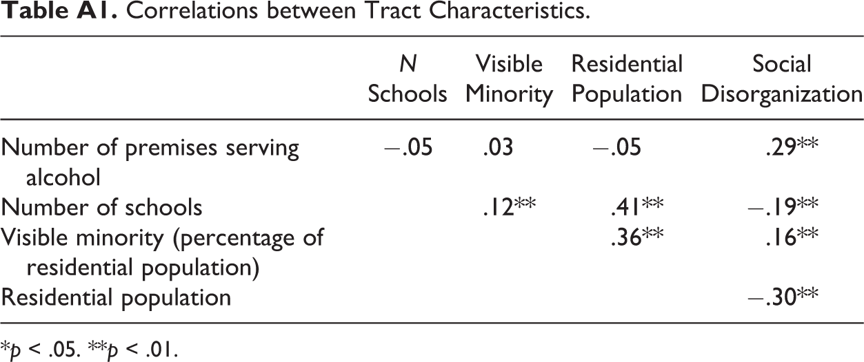
	N Schools	Visible Minority	Residential Population	Social Disorganization
Number of premises serving alcohol	−.05	.03	−.05	.29**
Number of schools		.12**	.41**	−.19**
Visible minority (percentage of residential population)			.36**	.16**
Residential population				−.30**

*p < .05. **p < .01.

Authors’ Note

A preliminary version of this article was presented at the 7th Illicit Networks Workshop in Montreal in November 2015.

Acknowledgments

The authors would like to thank Gisela Bichler and Carlo Morselli for their insightful comments as well as Joan McGilvray for her careful proof reading.

Declaration of Conflicting Interests

The author(s) declared no potential conflicts of interest with respect to the research, authorship, and/or publication of this article.

Funding

The author(s) received no financial support for the research, authorship, and/or publication of this article.

Notes

References

Anderson

James E.

Wincoop

Eric van

. 2004. “Trade Costs.” Journal of Economic Literature 42:691–751.

Andresen

Martin A.

Frank

Richard

Felson

Marcus

. 2014. “Age and the Distance to Crime.” Criminology & Criminal Justice 14:314–33.

Bernasco

Wim

. 2010. “A Sentimental Journey to Crime: Effects of Residential History on Crime Location Choice.” Criminology 48:389–416.

Bernasco

Wim

Block

Robert

. 2009. “Where Offenders Choose to Attack: A Discrete Choice Model of Robberies in Chicago.” Criminology 47:93–130.

Bernasco

Wim

Block

Robert

. 2011. “Robberies in Chicago: A Block-level Analysis of the Influence of Crime Generators, Crime Attractors and Offender Anchor Points.” Journal of Research in Crime and Delinquency 48:33–57.

Bernasco

Wim

Elffers

Henk

. 2010. “Statistical Analysis of Spatial Crime Data.” Pp. 699–724 in Handbook of Quantitative Criminology, edited by Piquero

A. R.

Weisburd

. New York: Springer.

Bernasco

Wim

Nieuwbeerta

Paul

. 2005. “How Do Residential Burglars Select Target Areas? A New Approach to the Analysis of Criminal Location Choice.” British Journal of Criminology 44:296–315.

Bichler

Gisela

Malm

Aili

Christie-Merrall

Jill

. 2011. “Urban Backcloth and Regional Mobility Patterns as Indicators of Juvenile Crime.” Pp. 118–36 in Patterns, Prevention, and Geometry of Crime, edited by Andresen

M. A.

Kinney

J. B.

Routledge Crime Science Series. Abingdon-on-Thames, England: Routledge.

Bichler

Gisela

Malm

Aili

Enriquez

Janet

. 2014. “Magnetic Facilities: Identifying the Convergence Settings of Juvenile Delinquents.” Crime & Delinquency 60:971–98.

10.

Bichler

Gisela

Christie-Merrall

Jill

Sechrest

Dale

. 2011. “Examining Juvenile Delinquency within Activity Space: Building a Context for Offender Travel Patterns.” Journal of Research in Crime and Delinquency 48:472–506.

11.

Boivin

Rémi

Felson

Marcus

. 2017. “Crimes by Visitors versus Crimes by Residents: The Influence of Visitor Inflows.” Journal of Quantitative Criminology, doi: 10.1007/s10940-017-9341-1.

12.

Boyce

Jillian

. 2015. “Police-reported Crime Statistics in Canada, 2014.” Juristat 35:Statistics Canada catalogue no. 85-002-X.

13.

Brantingham

Patricia J.

Brantingham

Paul L.

. 1993. Environment, Routine, and Situation: Toward a Pattern Theory of Crime. New Brunswick, NJ: Transaction.

14.

Brantingham

Paul L.

Brantingham

Patricia J.

. 2008. “Crime Pattern Theory.” Pp. 78–93 in Environmental Criminology and Crime Analysis, edited by Wortley

Mazerolle

. Portland, OR: Willan.

15.

Britt

Heather R.

Carlin

Bradley P.

Toomey

Traci L.

Wagenaar

Alexander C.

. 2005. “Neighborhood Level Spatial Analysis of the Relationship between Alcohol Outlet Density and Criminal Violence.” Environmental and Ecological Statistics 12: 411–26.

16.

Bruinsma, Gerben

J. N.

Pauwels

Lieven J. R.

Weerman

Frank M.

Bernasco

Wim

. 2013. “Social Disorganization, Social Capital, Collective Efficacy and the Spatial Distribution of Crime and Offenders: An Empirical Test of Six Neighborhood Models for a Dutch City.” The British Journal of Criminology 53:942–63.

17.

Burrows

John

Anderson

Simon

Bamfield

Joshua

Hopkins

Matt

Ingram

Dave

. 2001. Crime against Business in Scotland. Edinburgh, England: The Scottish Executive Central Research Unit.

18.

Clare

Joseph

Fernandez

John

Morgan

Frank

. 2009. “Formal Evaluation of the Impact of Barriers and Connectors on Residential Burglars’ Macro-level Offending Location Choices.” The Australian and New Zealand Journal of Criminology 42:139–58.

19.

Clarke

Ronald V.

(1999). “Hot Products: Understanding, Anticipating and Reducing Demand for Stolen Goods.” Police Research Series, Paper 112, Home Office, London, England.

20.

Cohen

Lawrence E.

Felson

Marcus

. 1979. “Social Change and Crime Rate Trends: A Routine Activity Approach.” American Sociological Review 44:588–608.

21.

Davies

Toby

Johnson

Shane D.

. 2015. “Examining the Relationship between Road Structure and Burglary Risk via Quantitative Network Analysis.” Journal of Quantitative Criminology 31:481–507.

22.

Desmarais

Bruce A.

Cranmer

Skyler J.

. 2012. “Statistical Inference for Valued-edge Networks: The Generalized Exponential Random Graph Model.” PLoS One 7:e30136.

23.

Elffers

Henk

Reynald

Danielle

Averdjik

Margit

Bernasco

Wim

Block

Richard

. 2008. Modelling crime flow between neighbourhoods in terms of distance and of intervening opportunities. Crime Prevention and Community Safety, 10:85–96.

24.

Felson

Marcus

. 2003. “The Process of Co-offending.” Pp. 149–68 in Theory for Practice in Situational Crime Prevention (Crime Prevention Studies, No. 16), edited by Smith

M. J.

Cornish

D. B.

. Monsey, NY: Criminal Justice Press.

25.

Frank

Richard

Andresen

Martin A.

Brantingham

Patricia L.

. 2012. “Criminal Directionality and the Structure of Urban Form.” Journal of Environmental Psychology 32:37–42.

26.

Graham

Kathryn

. 2009. “They Fight Because We Let Them! Applying a Situational Crime Prevention Model to Barroom Violence.” Drug and Alcohol Review 28:103–9.

27.

Graham

Kathryn

Jelley

Jennifer

Purcell

John

. 2005. “Training Bar Staff in Preventing and Managing Aggression in Licensed Premises.” Journal of Substance Use 10:48–61.

28.

Graham

Kathryn

Wayne Osgood

Wells

Samantha

Stockwell

Tim

. 2006. “To What Extent Is Intoxication Associated with Aggression in Bars? A Multilevel Analysis.” Journal of Studies on Alcohol 67:382–90.

29.

Gruenewald

Paul J.

Freisthler

Bridget

Remer

Lillian

Lascala

Elizabeth A.

Treno

Andrew

. 2006. “Ecological Models of Alcohol Outlets and Violent Assaults: Crime Potentials and Geographical Analysis.” Addiction 101:666–77.

30.

Hipp

John R.

Boessen

Adam

. 2013. “Egohoods as Waves Washing across the City: A New Measure of Neighborhoods.” Criminology 51:287–327.

31.

Johnson

Shane D.

Summers

Lucia

. 2015. “Testing Ecological Theories of Offender Spatial Decision Making Using a Discrete Choice Model.” Crime & Delinquency 61:454–80.

32.

Kinney

J. Bryan

Brantingham

Patricia L.

Wuschke

Kathryn

Kirk

Michael G.

Brantingham

Paul J.

. 2008. “Crime Attractors, Generator and Detractors: Land Use and Urban Crime Opportunities.” Built Environment 34:62–74.

33.

Land

Kenneth C.

McCall

Patricia L.

Nagin

Daniel S.

. 1996. “A Comparison of Poisson, Negative Binomial, and Semiparametric Mixed Poisson Regression Models: With Empirical Applications to Criminal Careers Data.” Sociological Methods & Research 24:387–442.

34.

Livingston

Michael

. 2008. “Alcohol Outlet Density and Assault: A Spatial Analysis.” Addiction 103:619–28.

35.

McFadden

Daniel

. 1986. “The Choice Theory Approach to Market Research.” Marketing Science 5:275–97.

36.

Nelson

A. L.

Bromley

R. D. F.

Thomas

C. J.

. 2001. “Identifying Micro-spatial and Temporal Patterns of Violent Crime and Disorder in the British City Centre.” Applied Geography 21:249–74.

37.

Pihl

Robert O.

Peterson

Jordan B.

. 1993. “Alcohol/Drug Use and Aggressive Behaviour.” Pp. 263–83 in Mental Disorder and Crime, edited by Hodgins

. Newbury Park, CA: Sage.

38.

Rengert

George F.

2004. “The Journey to Crime.” Pp. 169–181 in Punishment, Places and Perpetrators: Developments in Criminology and Criminal Justice Research, edited by Bruinsma

Ellfers

de Keijser

. Portland, OR: Willan.

39.

Rengert

George F.

Lockwood

Brian

. 2009. “Geographical Units of Analysis and the Analysis of Crime.” Pp. 109–22 in Putting Crime in Its Place: Units of Analysis in Geographic Criminology, edited by Weisburd

Bernasco

Bruinsma

G. J. N.

. New York: Springer.

40.

Rengert

George F.

Piquero

Alex R.

Jones

Peter R.

. 1999. “Distance Decay Re-examined.” Criminology 37:427–46.

41.

Rossmo

Kim D.

2000. Geographic Profiling. Boca Raton, FL: CRC Press.

42.

Sampson

Robert J.

Raudenbush

Stephen W.

Earls

Felton

. 1997. “Neighborhoods and Violent Crime: A Multilevel Study of Collective Efficacy.” Science 277:918–24.

43.

Schaefer

David R.

(2012). “Youth Co-offending Networks: An Investigation of Social and Spatial Effects.” Social Networks 34:141–9.

44.

Scott

John

. 2013. Social Network Analysis. 3rd ed. London, England: Sage.

45.

Shaw

Clifford R.

McKay

Henry D.

. 1931. Report on the Causes of Crime. Washington, DC: U.S. Government Printing Office.

46.

Stucky

Thomas D.

Ottensmann

John R.

. 2009. “Land Use and Violent Crime.” Criminology 47:1223–64.

47.

Sutherland

Edwin H.

1947. Principles of Criminology. 4th ed. Philadelphia, PA: Lippincott.

48.

Tinbergen

Jan

. 1962. Shaping the World Economy: Suggestions for an International Economic Policy. New York: Twentieth Century Fund.

49.

Townsley

Michael

Birks

Daniel

Ruiter

Stijn

Bernasco

Wim

White

Gentry

. 2016. “Target Selection Models with Preference Variation between Offenders.” Journal of Quantitative Criminology, 32:283–304 doi:10.1007/s10940-015-9264-7.

50.

Townsley

Michael

Sidebottom

Aiden

. 2010. “All Offenders Are Equal, but Some Are More Equal than Others: Variation in Journeys to Crime between Offenders.” Criminology 48:897–917.

51.

Van Koppen

Peter J.,

Keijser

Jan W. De

. 1997. “Desisting Distance Decay: On the Aggregation of Individual Crime Trips.” Criminology 35:505–15.

52.

Wang

Fahui

Arnold

Martin T.

. 2008. “Localized Income Inequality, Concentrated Disadvantage and Homicide.” Applied Geography 28:259–70.

53.

Weisburd

David

Groff

Elizabeth R.

Yang

Sue-Ming

. 2012. The Criminology of Place. Street Segments and Our Understanding of the Crime Problem. Oxford, England: Oxford University Press.

54.

Wilson

James D.

Denny

Matthew J.

Bhamidi

Shankar

Crammer

Skyler J.

Desmarais

Bruce A.

. 2017. “Stochastic Weighted Graphs: Flexible Model Specification and Simulation.” Social Networks 49:37–47.

55.

Zipf

George K.

(1949). Human Behavior and the Principle of Least Effort: An Introduction to Human Ecology. Cambridge, MA: Addison-Wesley Press.