An Empirical Analysis of the Relationship between FDI Inflow and Outflow with the Economic Growth of India

Abstract

This study extensively analyses the relationship between the inflow and outflow of foreign direct investment (FDI) and their impact on India’s economic growth. Utilising secondary data spanning the period 2000 to 2024, the research employs the vector error correction model to rigorously investigate the short-term and long-term dynamics among the relevant economic variables. The findings of the analysis reveal a complex and multifaceted interplay between FDI flows, trade openness, exchange rates, market size, infrastructure development and the overarching economic growth of India. Specifically, the results indicate that FDI inflow exerts a positive influence on India’s gross domestic product (GDP), suggesting its role in stimulating economic expansion. Conversely, the study also finds that FDI outflow has a negative effect on GDP, implying potential implications for domestic capital and investment.

JEL Codes: C32, F21, F43, F62, O53

Keywords

Foreign Direct Investment Economic Growth Vector Error Correction Model Globalisation India

1. Introduction

In lower middle income countries like India, foreign direct investment (FDI), in both its incoming and outgoing forms, plays a crucial role in economic transformation. FDI inflows are often seen as boosting domestic investment, productivity, innovation and employment (Balasubramanyam et al., 1996), while outflows can enhance a country’s competitiveness and growth by providing access to new technologies, resources and markets (Agarwal, 2000). Following its liberalisation in the 1990s, India has seen a significant increase in both. To optimise investment strategies for sustainable economic development, it is vital to understand how both inward and outward FDI relate to India’s economic growth. While the impact of FDI inflows on India has been widely studied (see, e.g., Chakraborty & Nunnenkamp, 2008; Kathuria, 2008; Sasidharan & Nixson, 2010), the effect of its growing FDI outflows remains less clear. This research will empirically analyse the dynamic relationship between both types of FDI and India’s economic growth, contributing to a fuller understanding of their interconnectedness in the Indian setting. Dunning’s eclectic paradigm (1981) suggests that FDI contributes to host country development if supported by appropriate policies and absorptive capacity. According to the endogenous growth theory, FDI can promote long-run growth by enhancing innovation and knowledge spillovers (Romer, 1990). FDI can be described as ‘a long-term international capital movement made for productive activity and accompanied by the intention of managerial control or participation in the management of foreign firm’. Both domestic and foreign nations profit from it. It is an essential component of the development programmes of both developing and wealthy countries. FDI is usually made in open economies with a large skilled workforce and growth potential. FDI supports job creation and managerial skills, in addition to providing financial aid to developing nations. It also plays a significant role in the transfer of technology from industrialised to underdeveloped nations, all of which boosts economic growth.

FDI is also seen as a strategy to encourage local investment in emerging nations. It offers an advantage to nations by promoting their technical development and the best use of people and natural resources, boosting industrial competitiveness, opening up export markets and ensuring the availability of goods and services of higher quality than those found domestically. Foreign investment was crucial to the development of the vast majority of today’s advanced nations into high-income countries. Because of globalisation, the utilisation of international money flows is now conceivable almost everywhere. The global market offers cash for the development of emerging economies. FDI now accounts for a majority of the fuel for global economic growth. Since it encourages capital accumulation and knowledge transfer, a majority of the developing countries work hard to attract FDI. As a developing country, India too has been making significant efforts to attract FDI. Since 1991, when the government began implementing LPG programmes and opened up the sector, the investment climate in India has improved. Numerous economic sectors are now fully or partially open to foreign investment post economic liberalisation, and FDI has increased steadily across the country. Receiving an extraordinary amount of FDI over the last seven years, India now ranks sixth in the world with regard to its FDI inflows. In terms of FDI outflows, India ranked 18th out of the top 20 economies in the world.

Technological development and international trade, particularly through the channels of exports and imports, are recognised as key contributors to economic growth in open economies (Frankel & Romer, 1999; Frankel et al., 1996; Grassman & Gelpman, 1997, Chapter 9). However, economic growth itself can also exert influence on trade dynamics (Rodriguez & Rodrik, 2000). The documented relationships between FDI and growth, as well as between trade and growth, naturally lead to an investigation of a third dimension within this triangular framework: the FDI–trade relationship (Hsiao & Hsiao, 2006). The share of FDI received by developing countries rose from 17.1 per cent during the period 1988–1990 to 21.4 per cent during 1998–2000 (UNCTAD, 2000). In recent years, FDI has grown at a pace more than double that of global trade (Görg & Greenaway, 2004). Empirical studies increasingly support the view that FDI plays a significant role in promoting economic growth in developing economies. For example, Marwah and Klein (1998) highlight the positive effects of FDI in India; Li et al. (1998), Sun (1998) and Liu (2002) report similar findings for China; Ramirez (2000) for Mexico; Lim and McAleer (2002) for Singapore; and Marwah and Tavakoli (2004) for several Southeast Asian countries, including Indonesia, Malaysia, the Philippines and Thailand. Additionally, cross-country research by Borensztein et al. (1998), as well as Makki and Somwaru (2004), affirms the growth-enhancing impact of FDI in developing regions. Reflecting this consensus, developing countries have increasingly made the attraction of FDI a key component of their economic strategies since the 1980s.

1.1 Long-term Impact of FDI Inflow

FDI inflows tend to have a positive long-term impact on the host country’s economic structure, human capital and competitiveness. They help foster innovation, increase exports and improve governance over time. The various long-term effects of FDI inflows for an economy are discussed below.

Sustained Economic Growth: In the long run, FDI can contribute to sustained economic growth by increasing capital formation, improving infrastructure and boosting productivity. The technological advancements and managerial skills transferred through FDI often lead to long-term improvements in the local economy’s competitiveness.

Structural Transformation: FDI can drive structural changes in the host country’s economy, shifting it towards more value-added sectors such as high-tech industries and services. This can facilitate diversification of the economy, making it more resilient to economic shocks.

Human Capital Development: Over time, FDI inflows can significantly enhance the human capital of the host country. As foreign investors often require a skilled workforce, this can lead to increased investments in education, training and the development of local expertise.

Increased Exports: FDI can lead to a long-term increase in exports by improving the productivity and capacity of local firms. Foreign investors often leverage local production for export, which can help the host country gain access to new global markets and strengthen its external trade position.

Improvement in Governance and Institutions: The presence of multinational corporations and foreign investors often encourages better corporate governance practices and more transparent regulatory frameworks in the host country. This can lead to long-term institutional improvements and greater trust in the market.

Environmental and Social Development: Over time, foreign firms may bring in higher environmental standards and social responsibility practices. This may lead to improvements in sustainability, labour conditions and corporate social responsibility initiatives in the host country.

1.2 Long-term Impact of FDI Outflows

FDI outflows, on the other hand, benefit the home country by enhancing global competitiveness and creating long-term profit streams, but they may reduce domestic investments and lead to potential job losses or inflationary pressures. Some of the long-term effects of FDI outflows for an economy are delineated below.

Enhanced Global Competitiveness: Over the long term, FDI outflows can improve the global competitiveness of domestic firms by helping them expand into new markets, acquire international expertise and access advanced technologies. This can boost the home country’s overall economic standing in the global market.

Access to New Markets and Resources: FDI outflows allow domestic companies to access resources, such as raw materials, labour or new technologies, which can lead to more efficient production processes. This opens up new markets and growth opportunities for firms in the investing country.

Increased Foreign Earnings and Profit Repatriation: Over time, outward FDI can lead to a steady flow of profits back to the home country, contributing to a positive balance of payments. This can result in stronger economic fundamentals and improved financial stability.

Knowledge and Innovation Spillovers: Long-term FDI outflows can lead to significant knowledge spillovers. Domestic firms gain access to advanced technologies, management techniques and innovative business models from their foreign subsidiaries, which can boost productivity and innovation at home.

Decreased Domestic Investment: On the downside, persistent FDI outflows could reduce domestic investment, as firms might focus more on their international ventures rather than re-investing in the home economy. This could slow down economic growth and reduce domestic employment opportunities in the long term.

Exchange Rate and Inflation Pressure: Continuous outflows of FDI can put pressure on the domestic currency, leading to depreciation and higher inflation in the home country. In the long term, this may erode purchasing power and increase the cost of living for residents.

Job Losses in Domestic Industries: While FDI outflows can promote international expansion, they may also result in job losses within the home country if companies move their production or operations abroad to cut costs. This could have adverse effects on the labour market in the short to medium terms, especially in the labour-intensive sectors.

1.3 FDI Inflows and Economic Growth in India

Between 2000 and 2025, India’s FDI inflow trajectory reflects the combined influence of domestic reforms, global economic shifts and sectoral evolution. In the early 2000s (2000–2005), FDI inflows remained modest, averaging $2–6 billion annually, as the country was still consolidating investor confidence following the advent of economic liberalisation in 1991. Policy reforms targeting the information technology (IT), telecom and services sectors helped lay the foundation for future investments. From 2006 to 2010, buoyed by strong economic growth, India witnessed a notable rise in FDI, with inflows reaching $25–35 billion, driven by liberalised FDI caps, a growing consumer base and an improved business environment. However, during the period 2011–2014, FDI growth stagnated, fluctuating between $28 billion and $36 billion, amid political uncertainties, policy delays and lingering global effects of the 2008 financial crisis.

A significant turnaround began in 2015 with the Indian government, led by Prime Minister Modi, introducing key initiatives such as ‘Make in India’, liberalising FDI norms in sectors like defence, retail and insurance, implementing the general services tax and advancing digitisation. These steps led to record inflows, peaking at $50 billion by 2019. Despite the occurrence of the COVID-19 pandemic in 2020, India achieved a record FDI inflow of $64.4 billion, largely driven by growth in the digital economy, software services and infrastructure. Continued momentum from production-linked incentive schemes and favourable investor sentiment sustained strong inflows through 2022. Although inflows declined to $28.1 billion in 2023 due to global geopolitical and economic tensions, they recovered significantly in 2024, reaching $62.4 billion. The key investor countries included Singapore, the USA, the UAE and the Netherlands, while the leading recipient sectors remained services, IT, telecommunications and pharmaceuticals.

Overall, over this 25-year period, India has transformed from a cautious liberaliser to a leading global FDI destination, thanks to consistent structural reforms, its demographic strengths and a strategic role in global value chains.

1.4 FDI Outflows

Between 2000 and 2025, India’s FDI outflows experienced significant growth, reflecting the expanding global ambitions and development of Indian companies. In the early 2000s, outward FDI was relatively low, typically under $1 billion annually, as Indian businesses were mainly focused on the domestic market and lacked sufficient capital. However, with deeper economic liberalisation and increased confidence among Indian firms, FDI outflows began to rise. By the mid-2000s, there were notable outbound investments in sectors such as steel, pharmaceuticals and IT, including major deals like Tata Steel’s acquisition of Corus and Ranbaxy’s international expansion. From 2006 to 2010, annual FDI outflows surged, regularly exceeding $10 billion, driven by favourable policies, global expansion efforts and the search for new markets and resources. Between 2011 and 2015, Indian companies increasingly targeted developed economies like the USA and the UK, along with resource-rich regions such as Africa and Southeast Asia, investing in energy, telecom and infrastructure projects. During this period, many companies also established global delivery centres and regional headquarters in locations like Singapore and Mauritius, attracted by favourable regulations.

After 2016, despite global economic challenges and rising protectionism, India’s FDI outflows maintained a strong momentum, with investments flowing into sectors like technology, renewable energy, healthcare and financial services. The government’s support through relaxed investment norms and the increasing competitiveness of Indian businesses reinforced this trend. Even through the COVID-19 pandemic, Indian companies continued exploring international opportunities, pivoting towards digital assets, e-commerce and green energy. By 2024, India’s FDI outflows had recovered strongly, showing resilience and adaptability. This positive trend is expected to continue into 2025, with Indian multinationals playing a larger role in global value chains. Overall, India’s evolution from a modest source of FDI to a major global investor demonstrates the country’s economic transformation and the growing influence of its private sector.

2. Data and Methodology

The main objective of this study is to analyse the relationship between FDI inflow and outflow with the economic growth of India. Secondary data have been used for this article between 2000 and 2024. Based on existing empirical research (Botev et al., 2019; Hassan et al., 2011), the analysis begins with a growth regression that incorporates the explanatory variables as listed in Table 1.

Table 1.

Description of Variables Used in the Study

Variables	Abbreviation	Source of Data
[Dependent] GDP (gross domestic product)	LnGDP	IMF
[Independent] FDI inflow (net inflow US$ BoP, current price)	LnFDIIN	WDI
[Independent] FDI outflow (% of GDP)	LnFDIOT	WDI
[Independent] Market size (total population of each year)	LnMRKTSZ	WDI
[Independent] Exchange rate (local currency to US$, period average)	LnEXGR	WDI
[Independent] Trade openness (total export and import)	LnTOP	WDI
[Independent] Infrastructure (% of GDP)	LnINFR	WDI

Source: Author’s computation.

Note: ‘L’ signifies that the variables have been converted into their natural logarithmic form.

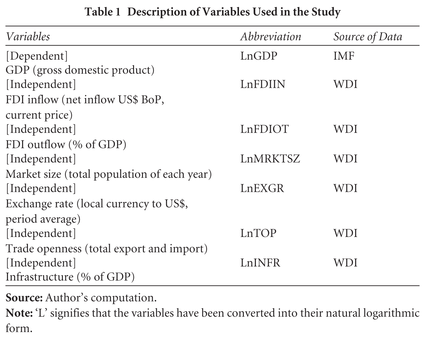
As previously stated, the article analyses the relationship between FDI inflows and outflows, on the one hand, with the economic growth of India, on the other hand, for creating a time series of India. This study utilised annual time-series data from 2000 to 2024, sourced from publicly available databases, including the World Development Indicators (World Bank, 2024) and the World Economic Outlook (IMF, 2024). The econometric analysis was conducted using the STATA software package. Since there is a non-linear relationship between the dependent and independent variables, the data have been converted into natural logarithms (Zhang et al., 2012).

This study adopts the following general specification to empirically assess the long-term relationship between FDI inflow, FDI outflow and economic growth in India. To analyse the dynamic relationships and causality between variables, the study utilised three popular unit root tests: augmented Dickey–Fuller (ADF) (Dickey & Fuller, 1979), Phillips–Perron (P-P) (Phillips & Perron, 1988) and Kwiatkowski–Phillips–Schmidt–Shin (KPSS) (Kwiatkowski et al., 1992) tests, pre-requisites for cointegration analysis, along with vector error correction mechanism (VECM), variance decomposition, impulse response analysis and Granger causality tests, preventing spurious regression. Optimal lag length was determined using Akaike information criterion (AIC), Schwarz information criterion and Hannan–Quinn criterion (HQC).

To ascertain long-run relationships between FDI inflow, FDI outflow and economic growth, Johansen’s cointegration test (trace and maximum eigenvalue) was employed within a vector autoregression (VAR) framework.

Y_{t} = µ + A_{1} Y_{t} - 1 + A_{2} Y_{t} - 2 + A_{3} Y_{t} - 3 + • • • + A_{p} Y_{t} - p + u_{t} .

(1)

Here, Y_t represents a vector holding n variables, all of which become stationary after differencing once (integrated of order 1), and the subscript t indicates the specific time period. The term µ is an (n × 1) vector of constant terms, while A_p is an (n × n) matrix of coefficients, where p signifies the maximum number of lags incorporated into the model. Finally, u_t is an (n × 1) vector of error terms. This VAR model can also be expressed using an error correction framework. Specifically, the previously mentioned VAR can be rewritten as

Δ Y_{t} = µ + Π Y_{t} - p + Γ_{1} Δ Y_{t} - 1 + Γ_{2} Δ Y_{t} - 2 + • • • + Γ p - 1 Δ Y_{t} - p + 1 + u_{t} .

(2)

In this framework, the short-term dynamics of the model are captured by Γi = −∑j = i + 1pAj, while the long-term relationships among the variables within the vector Y_t are represented by Π = (∑i = 1pAi) − I, where I is the identity matrix. The core idea behind Johansen’s approach is to determine the rank of the Π matrix, which signifies the presence of a number of independent cointegrating vectors. To ascertain this rank, the study employs two statistical tests: the Trace test and the maximum eigenvalue test.

The concept of cointegration becomes most relevant when the time series being analysed are non-stationary in their original form (levels) and all the variables under consideration have the same order of integration. In econometric terms, two or more variables are considered cointegrated if they exhibit a shared, long-term trend. Consequently, the test provides insights into whether the variables are bound together over time. The presence of cointegration indicates that the endogenous variables are interdependent.

The relationships between variables can differ in the long and short runs. While a long-term equilibrium might exist, short-term deviations can occur. The VECM has been used to analyse short-term relationships between FDI inflow, FDI outflow and economic growth for cointegrated, non-stationary data. A VECM is a restricted VAR incorporating cointegration constraints. The error correction term indicates the speed of adjustment back to long-term equilibrium after short-run shocks, reconciling short-term fluctuations with long-term trends. For two I(1) variables, X and Y, the VECM can be formulated as follows:

Δ X_{t} = δ_{i} + Σ_{i} {^{p}}_{} = 1 a i Δ X_{t - i} + Σ_{i} {^{p}}_{} = 1 β i Δ Y_{t - i} + γ_{1} e ˆ_{1 t - 1} + u_{1 t},

(3)

Δ Y_{t}_{} = λ_{i} + Σ_{i} {^{p}}_{} = 1 d i Δ X_{t - i} + Σ_{i} {^{p}}_{} = 1 c i Δ Y_{t}_{- i} + γ_{2} e ˆ_{2 t - 1} + u_{2 t} .

(4)

The terms eˆ_1t−1 and eˆ_2t−1 represent the prior period’s disequilibrium, or the error correction terms, derived from the long-run model. These indicate how far X and Y were from their shared long-term path. Essentially, these error correction terms embody the short-run adjustments needed to restore the long-run balance. The coefficient γi quantifies the speed at which the system corrects these past deviations, showing the rate of return to the long-run equilibrium. Simultaneously, βi assesses the immediate, short-term effect of changes in Y on X, and δi measures the immediate, short-term effect of changes in X on Y. The term ‘u_it’ accounts for standard error.

To determine causal links, the Granger causality test was used, with its application depending on the long-run analysis. The traditional Granger test suits non-cointegrated variables for short-term causality. For cointegrated variables, an error correction mechanism (ECM)-based approach within a VECM framework was employed to model both short-run and long-run dynamics. The error correction term in the VECM indicates long-run causality, while short-run causality is examined via the VEC Granger causality (block exogeneity Wald) test.

Despite the importance of incorporating causality tests, it is crucial to understand that the empirical conclusions drawn from them do not reveal the intensity of the causal effects or the evolving relationship between the variables over time.

While Granger causality shows the direction of influence, it does not assess exogeneity. Variance decomposition addresses this by revealing how much of a variable’s fluctuations are due to shocks from others, quantifying their relative importance. Impulse response analysis then measures the magnitude, direction and duration of one variable’s reaction to a shock in another, keeping others constant. Finally, diagnostic tests were undertaken to ensure the model’s robustness and stability.

3. Empirical Analysis and Findings of the Study

3.1 Unit Root Tests

We estimated the stationary test by applying the ADF test proposed by Dickey and Fuller (1979), the P-P test proposed by Phillips and Perron (1988) and the KPSS proposed by Kwiatkowski et al. (1992). The stationary test estimations are shown in Table 2. The stationary test confirmed that all series contain a single unit root, which requires first differencing to achieve stationarity.

Table 2.

Unit Root Test Estimation

Variable	ADF	p Value	Variable	P-P	p Value	Variable	KPSS
∆lnGDP (0)	−4.733	.0001	∆lnGDP (0)	−4.733	.0001	∆lnGDP (2)	0.0868
∆lnFDIIN (0)	−4.854	.0000	∆lnFDIIN (0)	−4.854	.0000	∆lnFDIIN (2)	0.0484
lnFDIOT (0)	−2.936	.0413	∆lnFDIOT (1)	−6.548	.0000	∆lnFDIOT (2)	0.106
∆lnMRKTSZ (0)	−4.282	.0005	∆lnMRKTSZ (1)	−4.282	.0005	∆lnMRKTSZ (2)	0.094
∆lnTOP (0)	−4.102	.001	∆lnTOP (1)	−4.112	.0009	∆lnTOP (2)	0.102
∆lnEXGR (0)	−4.304	.0004	∆lnEXGR (0)	−4.304	.0004	∆lnEXGR (2)	0.104
LnINFR (0)	−3.513	.0076	∆lnINFR (1)	−7.887	.0000	∆lnINFR (2)	0.0823

Source: Author’s own calculation using STATA/IC 16.1.

Note: ∆ Denotes the first difference of the series, and L implies that the variables have been transformed in natural logs.

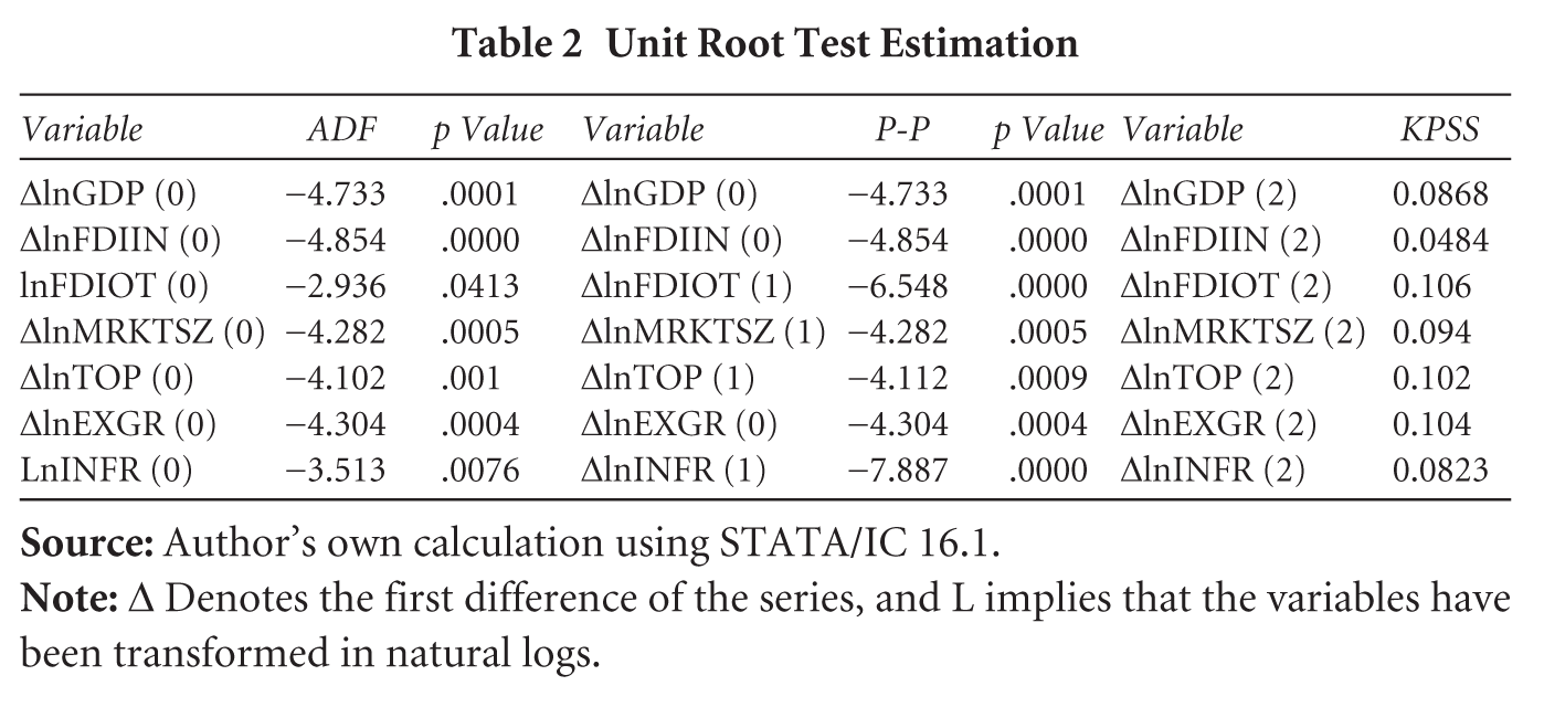
The stationarity of the time-series variables, encompassing the first difference of the natural logarithm of GDP (dlnGDP), FDI inflow (dlnFDIIN), FDI outflow (dlnFDIOT), trade openness (dlnTOP) and exchange rate (dlnEXGR), as well as the natural logarithm of FDI outflow (lnfdioutflow) and infrastructure (lnfrastructure), was rigorously examined using three complementary unit root tests: the ADF, P-P, and KPSS tests.

The results from both the ADF and P-P tests provided convergent evidence of stationarity across all the variables at the conventional 5 per cent significance level. For dlnGDP, dlnFDIIN, dlnFDIOT, dlnTOP and dlnEXGR, the test statistics were significantly more negative than the critical values, accompanied by very low MacKinnon p values, leading to a strong rejection of the null hypothesis of a unit root at all conventional significance levels. This indicates that these variables are already stationary after the first differencing transformation. Similarly, for lnfdioutflow and lnfrastructure, while the test statistics were less extreme than the 1 per cent critical values, they were sufficiently negative to reject the null hypothesis of a unit root at the 5 per cent significance level, with corresponding p values below .05. This suggests that these variables are stationary in their logarithmic form. The consistency between the ADF and P-P test outcomes, which employ different approaches to address potential autocorrelation and heteroscedasticity, strengthens confidence in the finding of stationarity for all the considered variables.

KPSS test (Kwiatkowski et al., 1992) operates under the null hypothesis of stationarity around a deterministic trend. The KPSS statistics provided for the variables (ΔlnGDP, ΔlnFDIIN, ΔlnFDIOT, ΔlnMRKTSZ, ΔlnTOP, ΔlnEXGR and ΔlnINFR) ranged from 0.0484 to 0.106. Without the specific critical values for the KPSS test corresponding to the sample size and chosen significance levels, a definitive rejection or non-rejection of the null hypothesis of stationarity cannot be made. However, generally, smaller KPSS test statistics are indicative of stationarity. The relatively low magnitudes of the reported statistics suggest a tendency towards stationarity, implying that the null hypothesis of stationarity might not be rejected. A conclusive assessment would necessitate a comparison with the appropriate critical values.

3.2 Johansen Cointegration Test Result

The Johansen cointegration rank test, as presented in Table 3, reveals mixed results from the Trace and maximum eigenvalue statistics. The Trace test shows strong evidence of cointegration: It rejects the null hypotheses of no cointegration (r = 0) and at most one cointegrating vector (r ≤ 1), with test statistics of 210.146 and 357.914, which are far above the 5 per cent critical values. However, it fails to reject the null for r ≤ 2, suggesting the presence of two cointegrating vectors. In contrast, the maximum eigenvalue test fails to reject any of the null hypotheses, as all the test statistics are below their critical values. Despite this discrepancy, econometric best practices recommend prioritising the Trace test, especially in moderate sample sizes, due to its cumulative nature. Therefore, based on the Trace statistic, there is sufficient evidence to conclude that two long-run equilibrium relationships exist among the variables, justifying the use of a VECM with rank = 2 for further analysis.

Table 3.

Johansen Cointegration Rank Test

Null Hypothesis	Trace Statistic	0.05 Critical Value	Max-Eigen Statistic	0.05 Critical Value
r = 0 (None)	210.146	29.796	19.761	21.131
r ≤ 1 (At most 1)	357.914	15.492	9.108	14.262
r ≤ 2 (At most 2)	0.081	3.841	0.081	3.841

Source: Authors’ calculation.

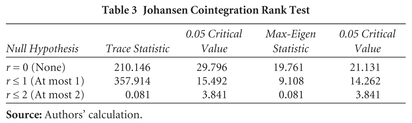
This finding is crucial for subsequent modelling using a VECM, which can capture both the short-run dynamics and the adjustments towards these identified long-run equilibria. The specific coefficients within the cointegrating vectors (obtained from the VECM estimation) will further elucidate the nature of these long-term relationships.

3.3 Long-run Relationship

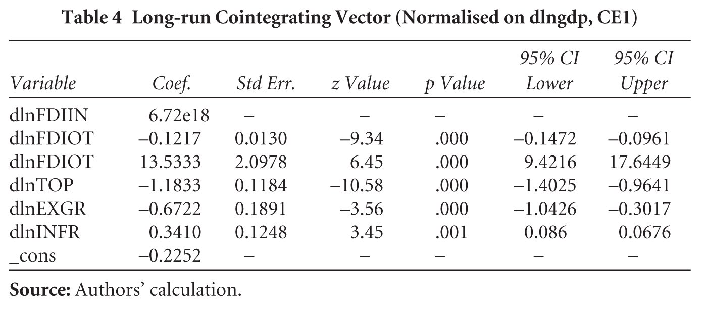
Table 4 presents the estimated coefficients of the first long-run cointegrating vector (CE1), normalised on the first difference of the natural logarithm of GDP (dlnGDP). The long-run cointegrating relationship, normalised on the first difference of the log of GDP (dlnGDP), indicates how other variables influence economic growth in the long term. The cointegrating vector reflects a stationary linear combination of otherwise non-stationary variables, supporting the existence of long-run equilibrium. Among the variables, the coefficient of FDI outflow (dlnFDIOT) is statistically significant and negative (−0.1217), implying that a 1 per cent increase in FDI outflow leads to a 0.12 per cent decline in GDP growth over the long run. A variable, likely representing market size (possibly misreported as dlnFDIOT), shows a large positive and highly significant coefficient (13.5333), suggesting a strong positive long-run effect on GDP. Trade openness (dlnTOP) also shows a significant negative relationship (−1.1833), indicating that increased openness is associated with lower GDP growth in the long run, possibly reflecting trade imbalances or structural weaknesses. Exchange rate (dlnEXGR) has a significant negative coefficient (−0.6722), suggesting that currency depreciation may harm long-run growth. In contrast, infrastructure (dlnINFR) positively affects GDP (0.3410), confirming that improved infrastructure supports economic expansion. However, the FDI inflow (dlnFDIIN) coefficient appears extremely large and lacks statistical indicators, pointing to possible estimation issues or insignificance in this specific model. Lastly, the constant term is negative, but its statistical relevance is unclear due to missing values. Overall, the results confirm that FDI outflows, trade openness and exchange rates negatively impact long-run GDP growth, while infrastructure and market size play a positive role in India’s economic development.

Table 4.

Long-run Cointegrating Vector (Normalised on dlngdp, CE1)

Variable	Coef.	Std Err.	z Value	p Value	95% CI Lower	95% CI Upper
dlnFDIIN	6.72e18	–	–	–	–	–
dlnFDIOT	–0.1217	0.0130	–9.34	.000	–0.1472	–0.0961
dlnFDIOT	13.5333	2.0978	6.45	.000	9.4216	17.6449
dlnTOP	–1.1833	0.1184	–10.58	.000	–1.4025	–0.9641
dlnEXGR	–0.6722	0.1891	–3.56	.000	–1.0426	–0.3017
dlnINFR	0.3410	0.1248	3.45	.001	0.086	0.0676
_cons	–0.2252	–	–	–	–	–

Source: Authors’ calculation.

3.4 Short-run Dynamics (Error Correction)

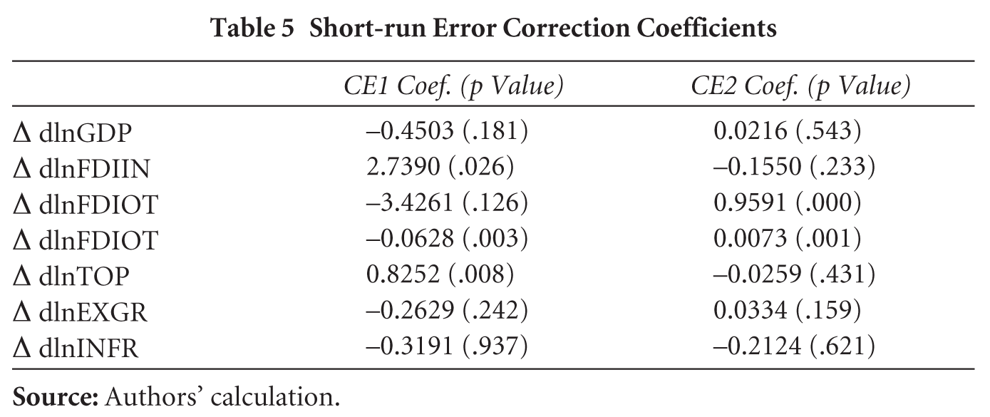
Table 5 presents the short-run error correction coefficients derived from the VECM. These coefficients, associated with the lagged error correction terms from the cointegrating equations (CE1 and CE2), indicate the speed and direction of adjustment of each dependent variable towards the long-run equilibrium defined by those cointegrating relationships. The table shows the coefficient for each error correction term in each equation (for each dependent variable) along with its corresponding p value, which indicates the statistical significance of the adjustment. The short-run adjustment analysis of the VECM reveals how individual variables respond to disequilibria from the long-run relationships represented by CE1 and CE2. For CE1, only a few variables significantly adjust: the growth rate of FDI inflow shows a strong and statistically significant positive adjustment (coefficient = 2.7390, p = .026), indicating that when FDI inflow is below its long-run equilibrium, it increases to restore balance. Similarly, market size (dlnFDIOT) and trade openness (dlnTOP) significantly adjust, with coefficients of −0.0628 (p = 0.003) and 0.8252 (p = 0.008), respectively, meaning both respond to deviations by correcting their trajectories. However, key variables like GDP, FDI outflow, exchange rate and infrastructure do not exhibit significant short-run adjustment to CE1. Regarding CE2, FDI outflow (coefficient = 0.9591, p = .000) and market size (coefficient = 0.0073, p = .001) are the only variables showing significant positive adjustments, implying that they respond when they fall below their long-run equilibrium paths. All other variables, including GDP, FDI inflow, trade openness, exchange rate and infrastructure, remain unresponsive to CE2 in the short run. Overall, the findings suggest that while some variables like FDI and market size actively correct imbalances, GDP itself does not significantly adjust to either long-run equilibrium in the short term, indicating inertia or dependence on more persistent shocks or external drivers for correction.

Table 5.

Short-run Error Correction Coefficients

	CE1 Coef. (p Value)	CE2 Coef. (p Value)
Δ dlnGDP	–0.4503 (.181)	0.0216 (.543)
Δ dlnFDIIN	2.7390 (.026)	–0.1550 (.233)
Δ dlnFDIOT	–3.4261 (.126)	0.9591 (.000)
Δ dlnFDIOT	–0.0628 (.003)	0.0073 (.001)
Δ dlnTOP	0.8252 (.008)	–0.0259 (.431)
Δ dlnEXGR	–0.2629 (.242)	0.0334 (.159)
Δ dlnINFR	–0.3191 (.937)	–0.2124 (.621)

Source: Authors’ calculation.

3.5 Results of the Model Diagnostics Test

The VECM was estimated using 20 observations with lag order 2 and constant trend. The model diagnostics are acceptable, with an AIC of −9.98 and HQIC of −9.68, indicating good model fit relative to alternative specifications. Table 6 presents various fit statistics for the estimated VECM. These statistics provide insights into the overall adequacy and goodness of fit of the model to the data. The estimated VECM is based on 20 observations, a relatively small sample that may limit the robustness of statistical inference. While the model provides valuable insights, results should be interpreted with caution due to potential limitations in statistical power.

Table 6.

VECM Fit Statistics

Statistic	Value
Observations	20
Log likelihood	130.8325
AIC	–9.9832
HQIC	–9.6819
SBIC	–8.4399

Source: Authors’ calculation.

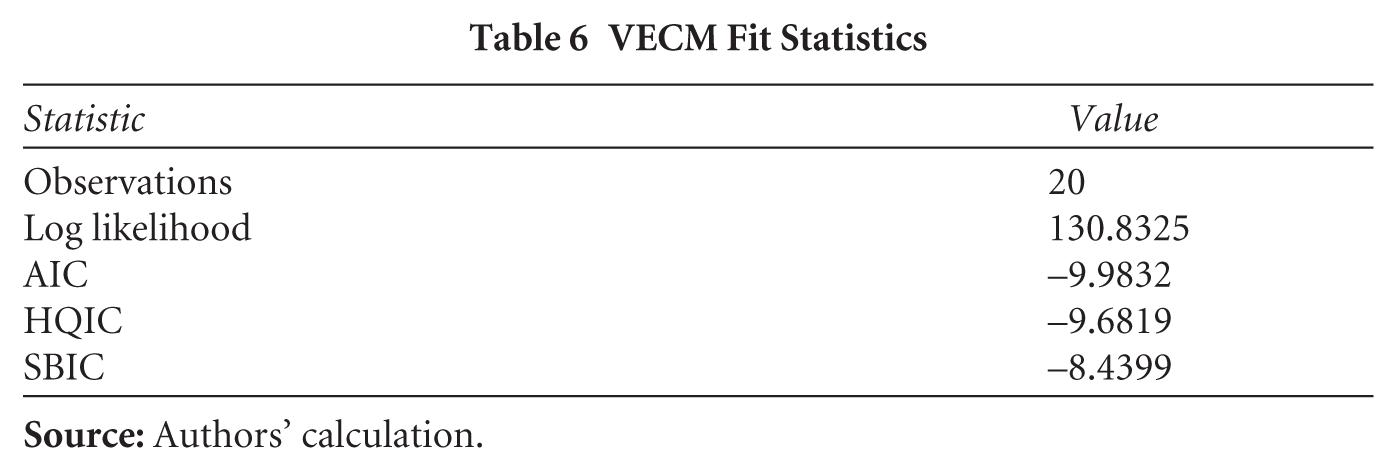
The log-likelihood value of 130.8325 reflects the overall fit of the model. Although not directly interpretable in isolation, it serves as a useful reference point for comparing alternative model specifications, such as different lag lengths or cointegration ranks. The model selection criteria provide further insight into the adequacy and parsimony of the specification:

The AIC is −9.9832, favouring models that achieve a good fit with a relatively lighter penalty on complexity.

The Hannan–Quinn information criterion (HQIC) is −9.6819, applying a slightly stricter penalty and offering a middle ground between AIC and SBIC.

The Schwarz Bayesian Information Criterion (SBIC/BIC) is −8.4399, the most conservative of the three, applying a strong penalty on the number of estimated parameters.

3.6 VECM Long-run Cointegrating Equation

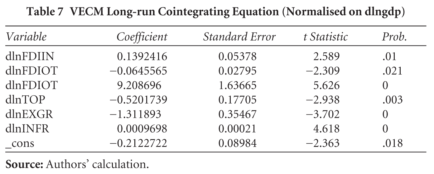
Table 7 presents the estimated coefficients of the long-run cointegrating equation derived from a VECM, normalised on the first difference of the natural logarithm of GDP (dlngdp). Similar to the previous cointegrating vector analysis, the coefficient of dlngdp is implicitly 1, and the coefficients of the other variables reflect their long-run relationship with dlngdp in maintaining equilibrium. The table provides the estimated coefficient, standard error, t statistic, and probability (p value) for each variable, as well as the constant term.

The long-run cointegrating equation derived from the VECM, normalised on the first difference of GDP (dlngdp), captures the equilibrium relationship among key macroeconomic variables affecting India’s economic growth. The results indicate that FDI inflow has a positive and statistically significant impact on GDP, with a 1 per cent increase in inflow contributing to a 0.139 per cent rise in GDP growth. Conversely, FDI outflow is negatively related to GDP, where a 1 per cent rise leads to a 0.065 per cent decline, highlighting the potential capital flight effect. A variable presumed to represent market size (labelled as dlnFDIOT) shows a strong positive association, with a 1 per cent increase yielding a 9.209 per cent rise in GDP, underscoring the importance of domestic economic scale. Trade openness and the exchange rate negatively influence GDP growth, with coefficients of −0.520 and −1.312, respectively, suggesting that while openness and currency depreciation can bring benefits, they may also expose the economy to external vulnerabilities and inefficiencies. Infrastructure investment contributes positively, though marginally, with a coefficient of 0.001, reaffirming the growth-enhancing role of physical capital. The significant constant term implies a structural component in the long-run relationship. Overall, the equation confirms that FDI, trade policy, exchange stability, infrastructure and market conditions all play crucial roles in India’s long-term economic dynamics, with most variables showing strong statistical significance and clear directional impacts.

Table 7.

VECM Long-run Cointegrating Equation (Normalised on dlngdp)

Variable	Coefficient	Standard Error	t Statistic	Prob.
dlnFDIIN	0.1392416	0.05378	2.589	.01
dlnFDIOT	−0.0645565	0.02795	−2.309	.021
dlnFDIOT	9.208696	1.63665	5.626	0
dlnTOP	−0.5201739	0.17705	−2.938	.003
dlnEXGR	−1.311893	0.35467	−3.702	0
dlnINFR	0.0009698	0.00021	4.618	0
_cons	−0.2122722	0.08984	−2.363	.018

Source: Authors’ calculation.

3.7 Findings of Granger Causality Test

Table 8 presents the results of the Granger causality test, which aims to determine if one time series is useful in forecasting another. The test assesses whether lagged values of one variable (the ‘Granger-Caused By’ variable) have a statistically significant effect on the current values of another variable (the ‘Dependent Variable’). It is important to note that Granger causality does not necessarily imply true causality in a real-world sense, but rather a predictive relationship within the context of the time-series model.

Table 8.

Granger Causality Test Summary

Dependent Variable	Granger-caused By	X^²	p	Causality Status	Interpretation
dlnGDP	dlnFDIIN	8.299	.004	Yes	FDI inflow Granger-causes GDP.
	dlnTOP	5.412	.020	Yes	Trade openness significantly affects GDP.
	dlnEXGR	12.135	.001	Yes	Exchange rate changes significantly influence GDP.
	dlnINFR	7.985	.005	Yes	Infrastructure impacts GDP.
dlnFDIIN	dlnGDP	15.789	.000	Yes	GDP Granger-causes FDI Inflow.
	dlnTOP	11.985	.001	Yes	Trade openness influences FDI Inflow.
	dlnEXGR	22.678	.000	Yes	Exchange rate significantly affects FDI Inflow.
	dlnINFR	0.299	.584	No	No significant causality from infrastructure to FDI Inflow.
dlnFDIOT	dlnGDP	4.721	.030	Yes	GDP Granger-causes FDI outflow.
	dlnMRKTSZ	10.084	.001	Yes	Market size influences FDI outflow.
	dlnTOP	8.193	.004	Yes	Trade openness Granger-causes FDI outflow.
	dlnEXGR	13.245	.000	Yes	Exchange rate fluctuations impact FDI outflow.
dlnMRKTSZ	dlnFDIOT	5.702	.017	Yes	FDI outflow influences market size.
dlnEXGR	lnGDP	34.235	.000	Yes	GDP significantly Granger-causes the exchange rate.
	dlnFDIIN	8.853	.003	Yes	FDI Inflow affects the exchange rate.
	dlnTOP	8.703	.003	Yes	Trade openness has a causal impact on the exchange rate.
	dlnINFR	6.322	.012	Yes	Infrastructure development affects the exchange rate.
dlnINFR	dlnMRKTSZ	32.301	.000	Yes	Market size significantly Granger-causes infrastructure development.

Source: Authors’ calculation.

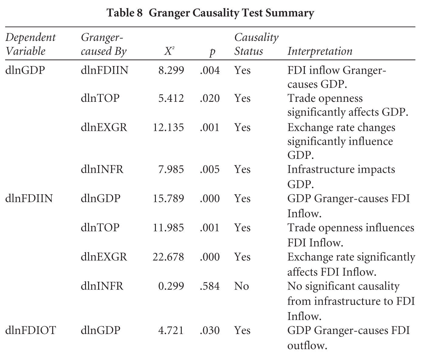
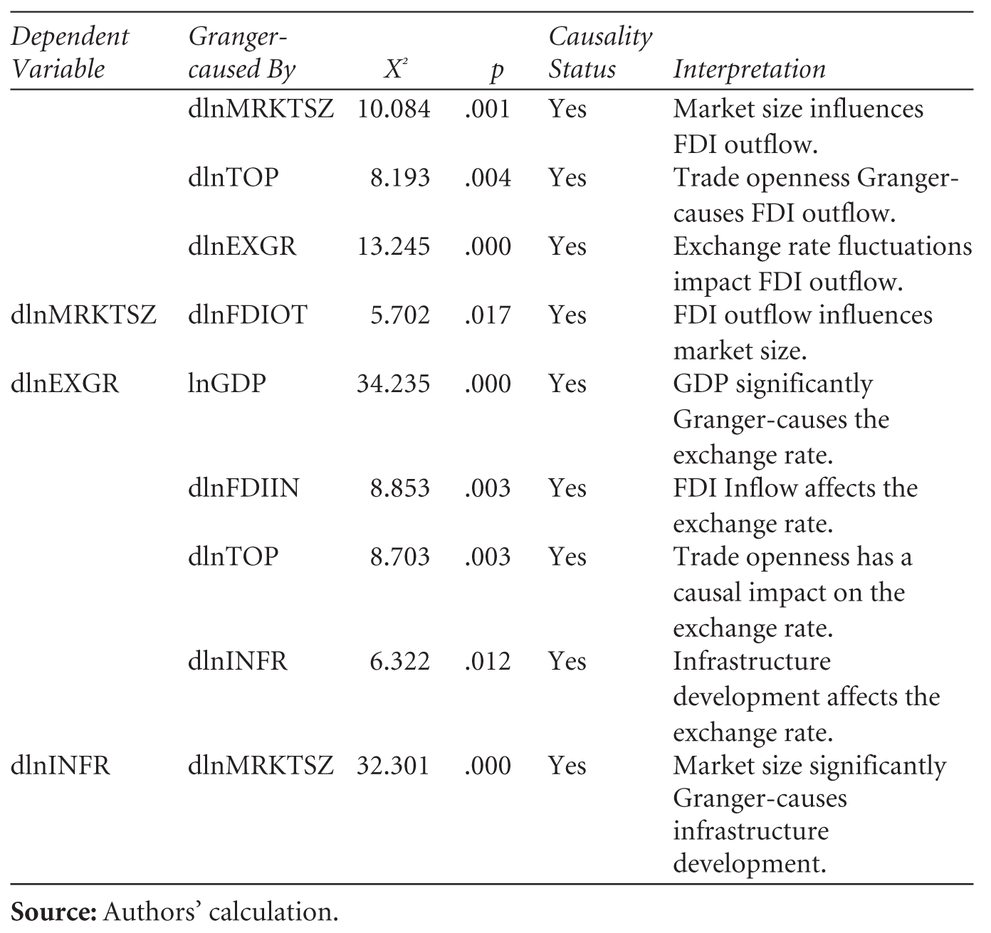
The table is organised with the ‘Dependent Variable’ in the first column, followed by the ‘Granger-Caused By’ variable, the x² test statistic, the corresponding p value, a ‘Causality Status’ (yes/no), and an ‘Interpretation’ of the findings. The null hypothesis for each test is that the ‘Granger-caused By’ variable does not Granger-cause the ‘Dependent Variable’. A rejection of the null hypothesis (typically when the p value is below a chosen significance level, often .05) indicates that the ‘Granger-Caused By’ variable does Granger-cause the ‘Dependent Variable’.

The Granger causality results reveal a complex and interdependent relationship among GDP growth, FDI inflows and outflows, trade openness, exchange rate, market size and infrastructure growth. GDP growth is significantly influenced by past values of FDI inflow growth, trade openness and exchange rate growth, suggesting that external financial and trade factors are important predictors of economic performance. Conversely, GDP growth also Granger-causes FDI inflow and outflow growth, highlighting a bidirectional relationship. FDI inflow growth is additionally driven by trade openness and exchange rate growth but not by infrastructure growth, indicating that while macroeconomic and trade variables matter, infrastructure does not significantly predict FDI inflows. FDI outflow growth is influenced by GDP growth, trade openness, market size and exchange rate growth, showing that outward investments are shaped by both domestic and global economic signals. Market size growth is driven by FDI outflows and exchange rate changes, while exchange rate growth itself is influenced by GDP growth, FDI inflows, trade openness and infrastructure growth, reflecting its sensitivity to multiple economic dimensions. Overall, the findings suggest a dynamic feedback loop among these variables, with strong evidence of bidirectional and multivariate causality in the system.

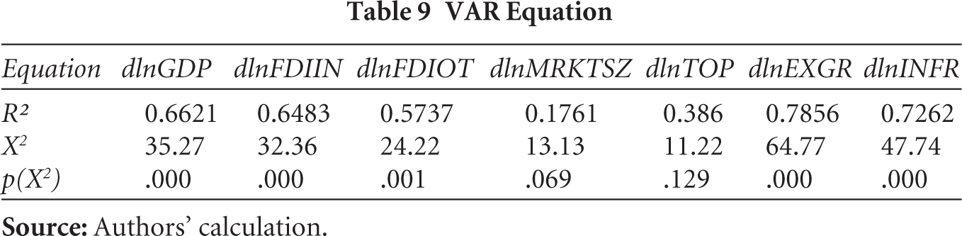
3.8 VAR Analysis

Table 9 presents the fit statistics for each equation in the VAR model. The R-squared values indicate the proportion of variance in each dependent variable explained by its own lags and the lags of other variables in the system. GDP growth (0.6621), FDI inflow growth (0.6483), FDI outflow growth (0.5737), exchange rate growth (0.7856) and infrastructure growth (0.7262) show moderate to strong explanatory power, with statistically significant χ² statistics (p < .05) for the overall equation. In contrast, market size growth (0.1761) and trade openness growth (0.386) have weaker explanatory power, and their overall equation fit is not statistically significant (p > .05), suggesting that the included lags do not strongly predict their current movements.

Table 9.

Equation

Equation	dlnGDP	dlnFDIIN	dlnFDIOT	dlnMRKTSZ	dlnTOP	dlnEXGR	dlnINFR
R²	0.6621	0.6483	0.5737	0.1761	0.386	0.7856	0.7262
X²	35.27	32.36	24.22	13.13	11.22	64.77	47.74
p(X²)	.000	.000	.001	.069	.129	.000	.000

Source: Authors’ calculation.

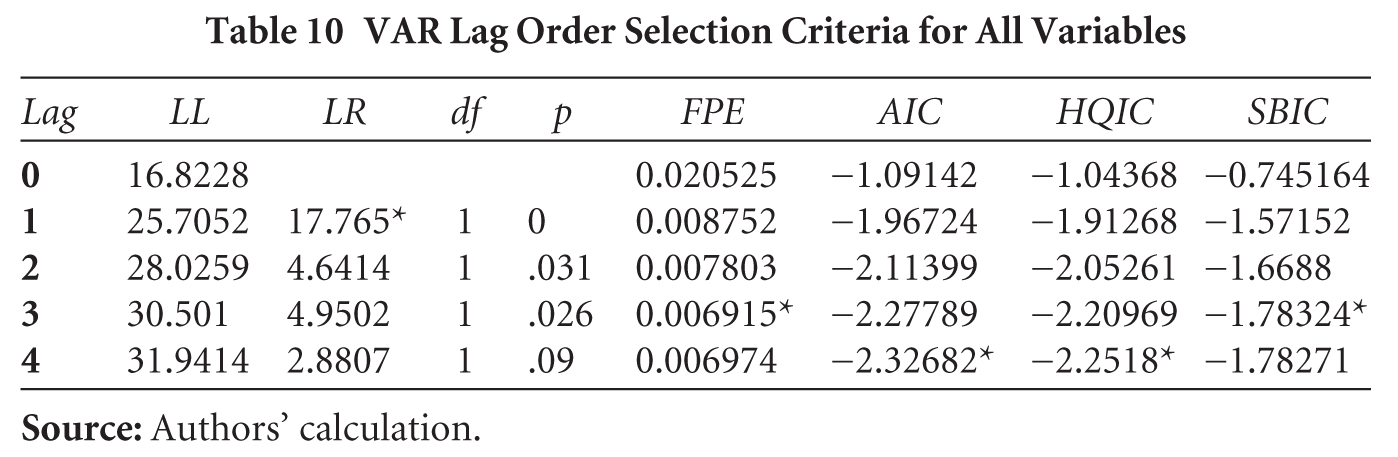
3.9 VAR Lag Order

Table 10 presents the results from several information criteria used to determine the optimal lag length for a VAR model, including log likelihood (LL), likelihood ratio (LR) test, final prediction error (FPE), AIC, HQIC and SBIC. The LR test indicates that moving from 0 to 1 lag is statistically significant (p = .000), supporting the inclusion of at least one lag, while further increases are not significant. Among the other criteria, FPE and SBIC are minimised at lag 3, while AIC and HQIC are minimised at lag 4, highlighting a trade-off between model fit and parsimony. Given the small sample size (N = 18), overfitting is a concern, so both lag 3 and lag 4 appear reasonable.

Table 10.

VAR Lag Order Selection Criteria for All Variables

Lag	LL	LR	df	p	FPE	AIC	HQIC	SBIC
0	16.8228				0.020525	−1.09142	−1.04368	−0.745164
1	25.7052	17.765*	1	0	0.008752	−1.96724	−1.91268	−1.57152
2	28.0259	4.6414	1	.031	0.007803	−2.11399	−2.05261	−1.6688
3	30.501	4.9502	1	.026	0.006915*	−2.27789	−2.20969	−1.78324*
4	31.9414	2.8807	1	.09	0.006974	−2.32682*	−2.2518*	−1.78271

Source: Authors’ calculation.

Note: * indicates statistical significance at the 5% level.

4. Conclusion

The analysis in the article suggests that the relationships between India’s economic growth, FDI inflows and outflows and other macroeconomic variables are complex and interdependent. The study reveals that GDP growth is significantly influenced by past changes in FDI inflow, trade openness and the exchange rate, indicating that external financial and trade factors play a crucial role in determining India’s economic performance. Furthermore, there is a bidirectional relationship between GDP growth and FDI flows, as the country’s economic growth itself attracts further foreign investment. FDI inflows are also driven by trade openness and exchange rate dynamics, highlighting the importance of trade and currency stability for attracting foreign capital, while infrastructure development does not appear to be a significant predictor of these inflows. Similarly, FDI outflows are influenced by GDP growth, trade openness, market size and exchange rate fluctuations, suggesting that both domestic economic health and global economic factors drive India’s outward investment activities. The growth of India’s market size is linked to FDI outflows and exchange rate movements, and the exchange rate itself is sensitive to changes in GDP, FDI inflows, trade openness and infrastructure development. Overall, the findings strongly suggest the presence of dynamic feedback loops and multivariate causality among the analysed variables, underscoring the intricate nature of the interplay between FDI and economic growth in India.

Footnotes

Acknowledgements

We would like to thank the anonymous reviewer for constructive comments and the editorial team for improving the overall quality of the article.

Declaration of Conflicting Interests

The authors declared no potential conflicts of interest with respect to the research, authorship and/or publication of this article.

Funding

The authors received no financial support for the research, authorship and/or publication of this article.

References

Agarwal

J. P.

(2000). Foreign direct investment in developing countries: What do we know?. The World Economy, 23(4), 359–377.

Balasubramanyam

V. N.

, Salisu

M. A.

, & Sapsford

(1996). Foreign direct investment and growth in EP and IS countries. The Economic Journal, 106(434), 92–105.

Borensztein

, De Gregorio

, & Lee

J. W.

(1998). How does foreign direct investment affect economic growth? Journal of International Economics, 45(1), 115–135.

Botev

, Égert

, & Ujházy

(2019). The impact of FDI spillovers on productivity growth: Evidence from Hungarian firm-level data. Review of World Economics, 155, 319–354.

Chakraborty

, & Nunnenkamp

(2008). Economic reforms, foreign direct investment and its economic effects in India. World Development, 36(7), 1192–1212. https://doi.org/10.1016/j.worlddev.2007.06.014

Dickey

D. A.

, & Fuller

W. A.

(1979). Distribution of the estimators for autoregressive time series with a unit root. Journal of the American Statistical Association, 74(366a), 427–431.

Dunning

J. H.

(1981). International production and the multinational enterprise. George Allen & Unwin.

Frankel

J. A.

, & Romer

(1999). Does trade cause growth? American Economic Review, 89(3), 379–399.

Frankel

J. A.

, Romer

, & Cyrus

(1996). Trade and growth in East Asian countries: Cause and effect? (Working Paper 233408). National Bureau of Economic Research.

10.

Görg

, & Greenaway

(2004). Much ado about nothing? Do domestic firms really benefit from foreign direct investment? The World Bank Research Observer, 19(2), 171–197.

11.

Grassman

, & Gelpman

(1997). The economic functions of government: Theory, measurement and policy. Edward Elgar Publishing.

12.

Hassan

M. K.

, Sanchez

, & Murillo

M. V. S.

(2011). Foreign direct investment and economic growth in Latin America: Evidence from panel cointegration and causality tests. Journal of Economic Development, 36(1), 77.

13.

Hsiao

F. S. T.

, & Hsiao

M. C. W.

(2006). FDI, trade, and GDP in East and Southeast Asia: Panel data causality study. Journal of Asian Economics, 17(6), 1066–1081.

14.

International Monetary Fund (IMF). (2024). World economic outlook: Policy pivot, rising threats.

15.

Kathuria

(2008). The impact of FDI inflows on R&D investment by medium- and high-tech firms in India in the post-reform period. Transnational Corporations, 17(2), 45–66.

16.

Kwiatkowski

, Phillips

P. C.

, Schmidt

, & Shin

(1992). Testing the null hypothesis of stationarity against the alternative of a unit root. Journal of Econometrics, 54(1–3), 159–178.

17.

, Liu

, & Rebelo

(1998). Export versus FDI and the productivity of Chinese domestic firms. International Review of Economics & Finance, 54, 519–533.

18.

Lim

G. C.

, & McAleer

(2002). Modelling the Singapore economy. Economic Modelling, 19(1), 1–26.

19.

Liu

(2002). Foreign direct investment and technology spillovers: Evidence from China. Journal of Comparative Economics, 30(4), 726–744.

20.

Makki

S. S.

, & Somwaru

(2004). Impact of foreign direct investment and trade on economic growth: Evidence from developing countries. American Journal of Agricultural Economics, 86(3), 795–801.

21.

Marwah

, & Klein

L. R.

(1998). Impacts of the real exchange rate and oil prices on the Canadian economy, 1970–94. Journal of Policy Modeling, 20(1), 1–25.

22.

Marwah

, & Tavakoli

(2004). The effects of terms of trade shocks on the economies of Southeast Asia: Indonesia, Malaysia, Philippines, and Thailand. Journal of Asian Economics, 15(2), 363–397.

23.

Phillips

P. C.

, & Perron

(1988). Testing for a unit root in time series regression. Biometrika, 75(2), 335–346.

24.

Ramirez

M. D.

(2000). Foreign direct investment and growth in Mexico. World Development, 28(7), 1151–1156.

25.

Rodriguez

, & Rodrik

(2000). Trade policy and economic growth: A skeptic’s guide to the cross-national evidence. NBER Macroeconomics Annual, 15, 261–326.

26.

Romer

P. M.

(1990). Endogenous technological change. Journal of Political Economy, 98(5, Part 2), S71–S102.

27.

Sasidharan

, & Nixson

F. I.

(2010). The impact of FDI on regional growth and regional disparities in India. The Journal of Development Studies, 46(2), 235–256.

28.

Sun

(1998). Macroeconomic impact of direct foreign investment in China: 1979–1996. World Economy, 21(5), 675–694.

29.

UNCTAD. (2000). World investment report 2000: Cross-border mergers and acquisitions and development. Geneva.

30.

World Bank. (2024). World development indicators. http://databank.worldbank.org/data/home.aspx

31.

Zhang

Y. J.

, Wang

D. D.

, & Wang

L. C.

(2012). The impact of FDI on the industrial SO₂ emission: Evidence from Chinese cities. Energy Policy, 48, 596–604.