
Abstract
Objective
We aimed to evaluate whether the internal structures of the human ear have anatomical characteristics that are sufficiently distinctive to contribute to human identification and use in a forensic context.
Materials and methods
After data anonymisation, a dataset containing temporal bone CT scans of 100 subjects was processed by a radiologist who was not involved in the study. Four reference images were selected for each subject. Of the original sample, 10 examinations were used for visual comparison, case by case, against the dataset of 100 patients. This visual assessment was performed independently by four observers, who evaluated the anatomical agreement using a Likert scale (1–5). Inter-observer agreement, true positive rate, positive predictive value, true negative rate, negative predictive value, false positive rate, false negative rate and positive likelihood ratio (LR+) were evaluated.
Results
Inter-observer agreement obtained an overall Cohen’s Kappa = 99.59%. True positive rate, positive predictive value, true negative rate and negative predictive value were all 100%.
Conclusion
Visual assessment of the mastoid examinations was shown to be a robust and reliable approach to identify unique osseous features and contribute to human identification. The statistical analysis indicates that regardless of the examiner’s background and training, the approach has a high degree of accuracy.
Introduction
Computed tomography (CT) is a method of medical imaging that has high spatial and contrast resolution. Accordingly, it can be used to recognise and evaluate small osseous features of the middle ear, inner ear, mastoid process, sutures and the base of the cranium.
Nowadays, CT scanning data are archived in digital systems that are capable of storing medical examination records for periods of longer than 10 years. In addition, many institutions provide compact discs to their patients that include data acquired during their clinical examinations, thereby allowing them to maintain their own information for an unspecified period.1–3
In the specific case of the temporal bone, the differences between bone structures and the surrounding air, along with the inherent anatomical complexity of the area (Figure 1), indicate that it might be an ideal area in which to find criteria for identification that are both individualising and immutable following the end of bone maturation.4,5
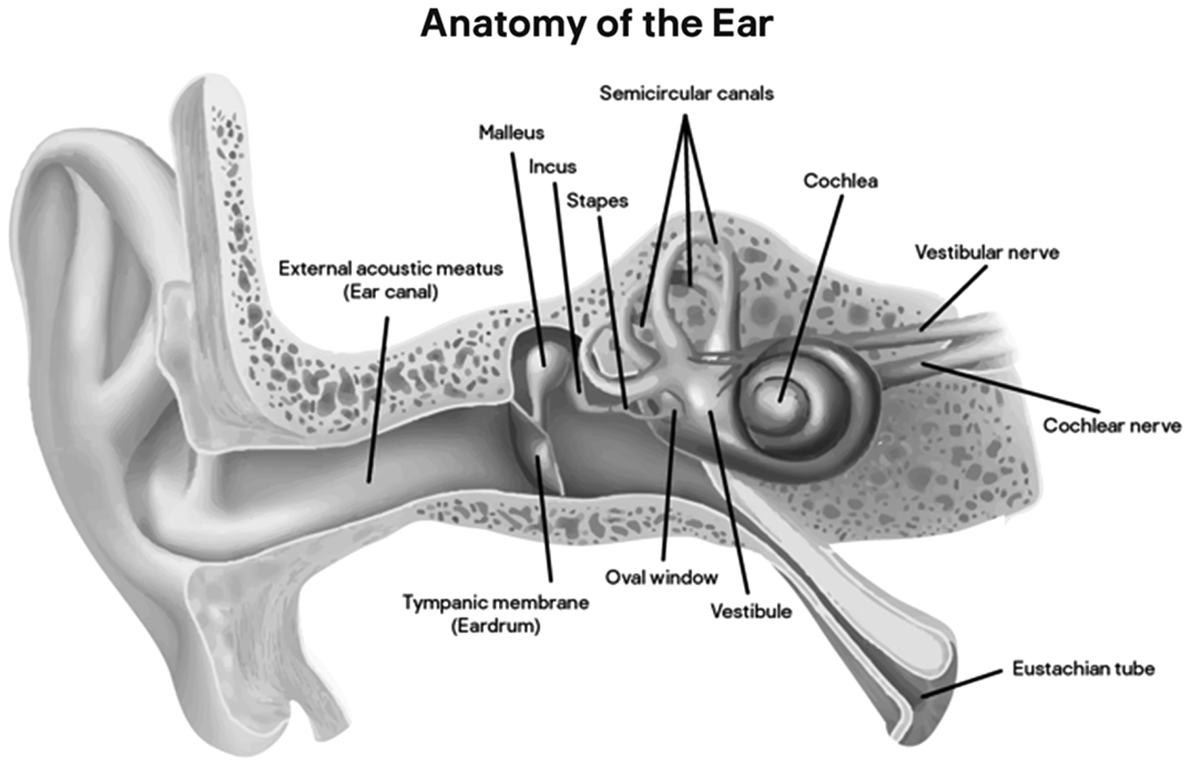
Anatomic drawing of the human ear, with the reference points used.
In addition, the temporal bone is a highly resistant anatomic structure. Its internal structure is commonly found intact in cadaveric remains, even when it has been subjected to considerable trauma, high thermic amplitude, or when it is evaluated many years after death: studies using CT scans indicate that only the ossicular chain suffers severe structural alterations when the ear is filled by soil.6,7
There are many studies validating the evaluation of osseous structures by radiography or CT scan as methods of post-mortem identification. Of these, the best known are based on an evaluation of the frontal sinus, which presents a confidence level for identification that is similar to a fingerprint.8–14
For an expert’s report to be valid in court, it must use methods that are statistically supported, peer-reviewed, published and reproducible. One of the most pertinent discussions within the scope of forensic sciences is to determine how many concordance points are mandatory in order to satisfy the assumption that a specific anatomic feature can, with very high probability, belong to one, and only one, individual.15–17
Thus, attempting to validate identification criteria using morphological analyses of specific structures is tempting. In this regard, the temporal bone is likely to be of importance within forensic anthropology in particular, and the forensic sciences in general. It has the potential to offer useful insights in the contexts of mass disasters, crimes against humanity, the identification of missing people and other relevant medico-legal problems.18–20
CT scanners are highly performant these days, and an acquisition made after death for forensic purposes could always be post processed to match ante-mortem parameters of images, since the raw data in the PACS (Picture Archiving and Communication System) stations can be reconstructed with excellent quality with any slice thickness and in any plane is desired, for later comparison between images in different time sets.
Imaging algorithms also should not be a problem because most vendors use similar kernels, and matrix of acquisition and dose are standardised to ensure high-quality images. In this way, we could arrange to match image displays before and after death.
Our aim with this project was to evaluate the internal structure of the temporal bone, using independent observers to determine if CT scans of the temporal bone can be used as a simple and statistically valid method for human identification, with applicability in real forensic scenarios.
Materials and methods
After obtaining approval from the ethic commission of the University of Coimbra, an aleatory sample was obtained to proceed with the study. The authors used the digital archive of CHUC’s (Coimbra Universitary Hospital Centre) Radiology Department, to randomly choose 100 examinations of CT scans of the ears performed during the year 2015.
These examinations were acquired with a Siemens Somaton Emotion®, with 16 detectors, FOV (Field of View) adapted to the region of interest, 512 × 512 matrix, HP90 ultra-sharp algorithm for reconstruction, 0.6 mm collimation and image reconstruction with 0.75 mm of effective thickness, using 0.5 pitch, 130 KV (Kilovolts) and 220 mAs (milliamperes/second).
The sample contained 50 men and 50 women, with an age range of 20–90 years old. In the filtering process, only examinations that had the totality of the images, allowing for reconstruction of multi-planar images, acquired through a standardised technical protocol were considered, regardless of whether they did or did not have pathological processes affecting the structural morphology in a transitory or definitive manner.
After anonymisation and elimination of all identification tags, the sample was processed by a radiologist, who reconstructed axial and coronal reference images, but was not involved with the image observation study. This work was done by a single medical doctor, with the aim of eliminating discrepancies between images included in the study that could hamper the readers’ work and save time. Since detailed comparisons of small morphologic structures rely upon strict plan comparisons, that seemed more feasible to us. Despite this choice of method, we provided strict criteria for this selection, and reference images could be reproduced by any radiologist or forensic expert that needs to use or test the method.
Four reference images were selected, one axial and the other three in a coronal plane. All corresponded to the most stable anatomical planes that could clearly be established in all patients of the sample. All the images were reconstructed using the same algorithm and were visualised with the same window.
The study’s coordinator previously prepared the reference images, using the 3D tool of the OSIRIX software and determined the axial image, based on a plane that went through the external semicircular canal foramens, and the coronal images perpendicular to the axial image selected as reference.
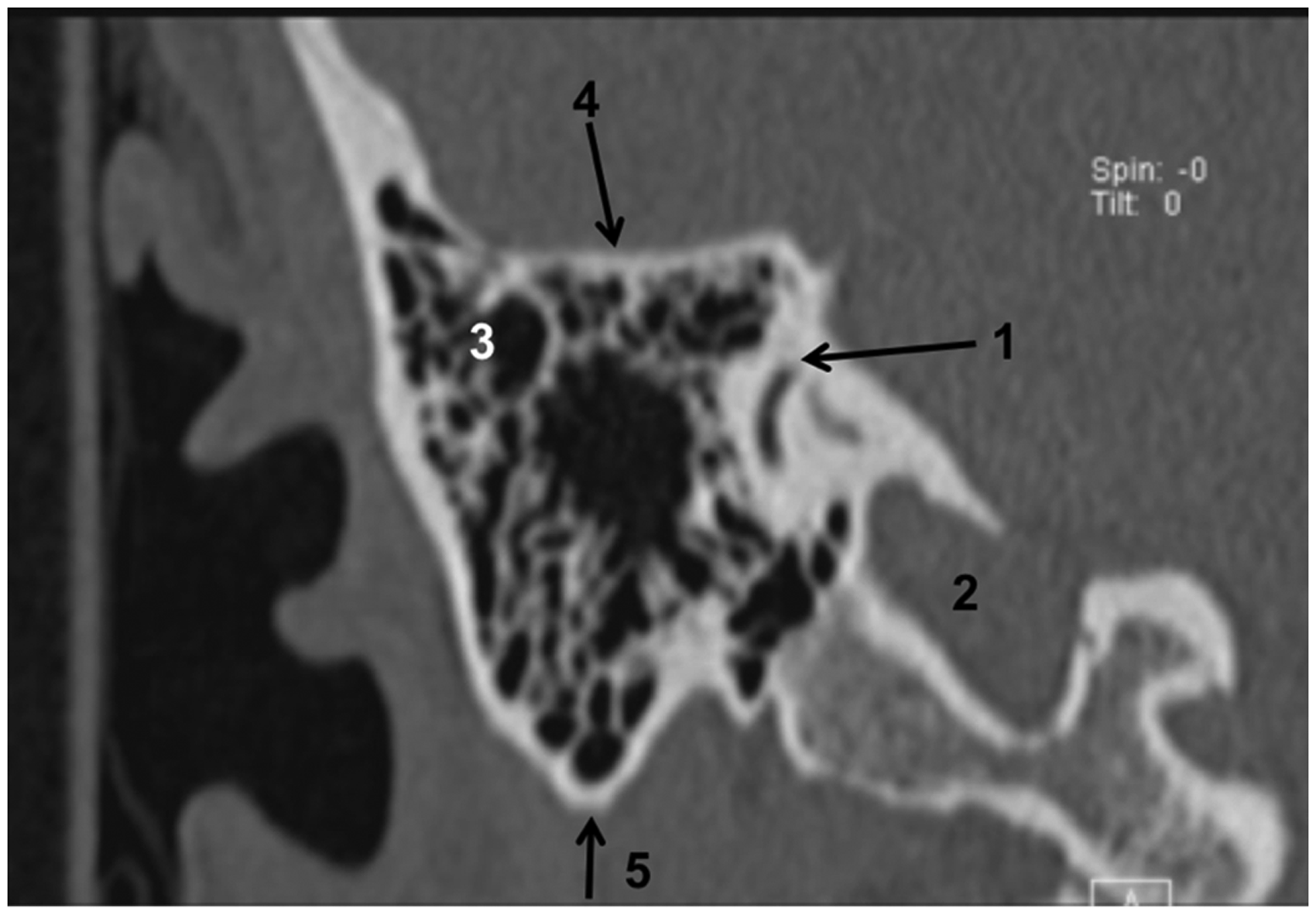
The selected axial image was the plane where the greatest extension of the external semicircular canal, with a ‘c’ morphology, could be observed, preferentially identifying the anterior and posterior communication with the vestibule (Figure 2).
Reference axial image.
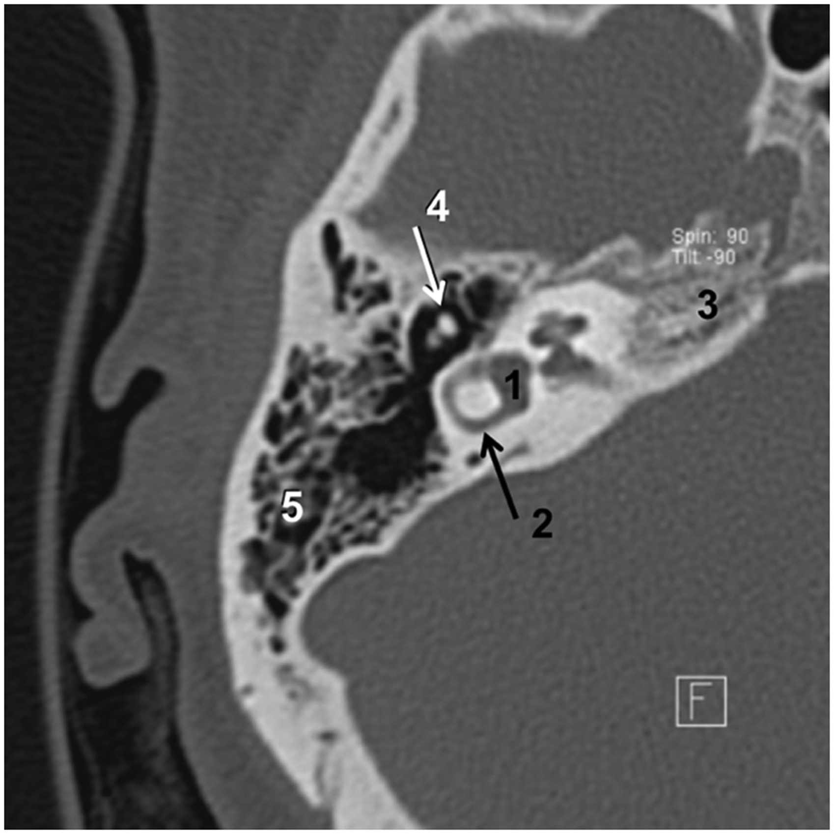
The three coronal images were based on different reference points: in the first we selected the plane where the internal auditory meatus could be observed at the crista falciformis level and the cochlear nerve entrance point (Figure 3); in the second one we selected the plane where the apex and the first turn of the cochlea could be depicted, clearly defining the thin osseous blade that separates both structures (Figure 4); in the third, we selected the plane where the contour of the posterior semicircular canal is longest (Figure 5).
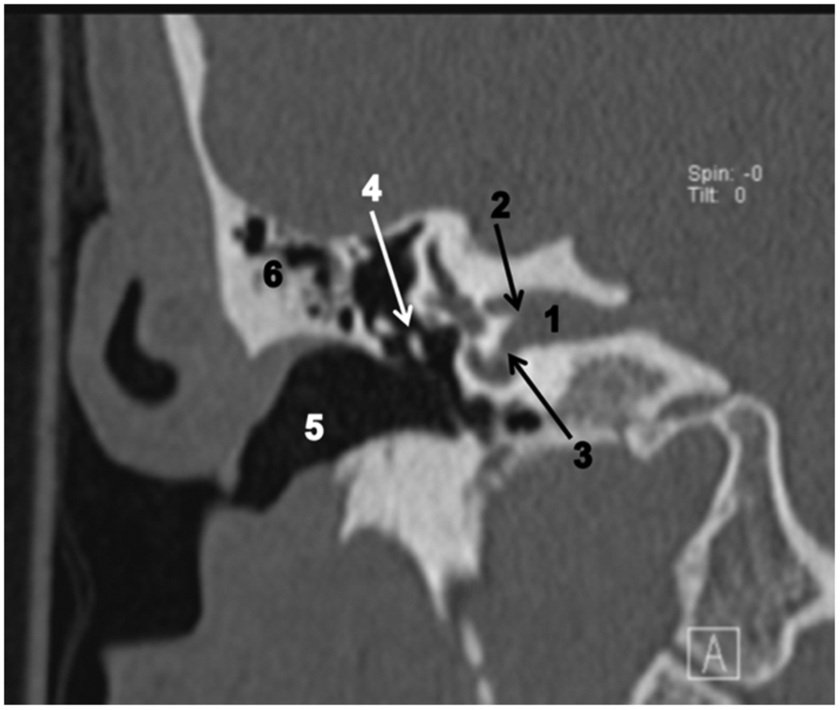
Reference coronal image 1.
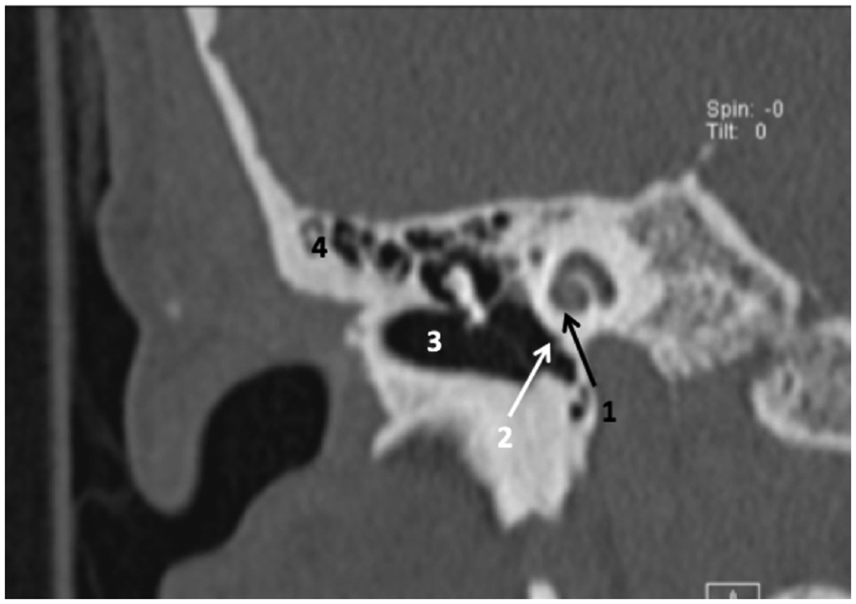
Reference coronal image 2.
Reference coronal image 3.
The aim of this selection, based on anatomical references, is to allow these planes to be reproducible in forensic acquisitions and reconstructed by digital post-processing. They also have the advantage of decreasing the disparities in background training of the different observers. This allows those less familiarised with CT scans to classify the imagery with confidence. It also decreases the time, since it does not require observers to review a full CT study, an aspect that could lead to observer fatigue.
During image review, the observers did not have any time limitations, and were accompanied by an investigator who registered the reader observations according to the Likert scale, and had no knowledge of the correspondences.
The observers were asked to meet the following criteria in reference images:
Axial image:
Contour, density and pneumatisation of the petrous apex. Internal contour of the middle ear cavity. Contour and dimension of the sigmoid sinus. Morphology, dimension and organisation of the mastoid cells. Relative position of the vestibule and the cochlea.
Coronal image 1:
Organisation of the mastoid cells laterally to the epitympanum. Density, contour and bone morphology superior to the internal auditory canal. Density, contour and bone morphology inferior to the internal auditory canal. Thickness and contour of the tegmen tympani. Contour, density and bone structure inferior to the external auditory canal.
Coronal image 2:
Morphology of the mastoid cells adjacent to the tegmen tympani. Extension and contour of the hyperdense area around the cochlea. Relative orientation of the external auditory canal in relation to the cochlea. Contour, density and structure of the internal petrous contour. Contour, density and internal architecture of the mastoid inferior to the external auditory canal.
Coronal image 3:
Contour and thickness of the mastoid’s cortex. Morphology and dimension of the sigmoid sinus. Morphology of the mastoid cells adjacent to the mastoid tegmen. Shape and pneumatisation of the petrous apex. Morphology, contour and dimension of the biggest mastoid cell.
For the observations by the readers, we used two MacBook Pro computers, with 15-inch screens, placed side by side, utilising the OSIRIX software to visualise the CT images.
To one of them, 40 reference images of the 10 problem cases were downloaded. In the other were the 400 reference images (four groups of 100 images) of the population chosen as samples.
On one of the computers, the assistant displayed one of the problem images, while on the other the reader scrolled through all 100 correspondent images of the sample, to perform the classification in accordance with the reference points in the Likert scale. The observers were told to establish the agreement using a Likert scale (1–5) according to their level of confidence in their interpretation. 21
These observations were independent and blind. In terms of the classification scale, further details of which can be found in Table 1, it was determined that 1 would mean total absence of agreement, while 5 would mean total agreement.
Classification criteria provided to the observers, based on a Likert scale.
Later, for statistical analysis, we considered a rate of 5 as perfect match and all other rates as a non-correspondence, to permit the interpretation as a binary scale.
The dataset was read by four observers with different experiences and independently: (a) a medical doctor with over 10 years of experience in radiology; (b) another medical doctor, with over 2 years of experience in neuroradiology; (c) a medical imaging technician; (d) an anthropologist who has had only 2–6 hours of training in CT scans observations, in order to evaluate if he could recognise major anatomical features.
We did not use the subtraction or fusion tools in the workstation for three main reasons. First, we had the objective to compare the performance between radiologists and non-radiologists, and the use of this kind of instrument would introduce a bias for those not familiar with managing these workstation tools. The second reason relates to technical problems, since small differences in field of view and image orientation would have produced dubious results, and would be very time consuming to manage. This is because in the area of ear anatomy, we are evaluating very thin osseous structures, surrounded by air, with big differences in density interfaces. Third, for our perspective of application in real-case scenarios, where pre- and post-mortem images might have been acquired by different scanners, with slightly different image kernels, dose, field of view and soft tissue contribution, workstation evaluation would add extra difficulties, that could be surpassed with success by human observation.
To perform all statistical analysis, the R statistical language was used. 22 Whenever the denominator was zero, to avoid infinity, the lowest float-point represented by the R system was assumed. We intended to verify if the four observers could match the real individual in four different planes for each of the 10 problem cases to their counterparts on the sample of 100 individuals.
Then, we intended to verify if the background of the observers influenced their evaluations, in order to assess if the method could be easily learned, applied and reproduced. For that, we calculated the inter-observer agreement and the reliability of agreement through Fleiss’ Kappa, adapted for ordered-categorical data.
Other performance metrics such as the true positive rate (sensitivity, recall), positive predictive value (precision), true negative rate (specificity), negative predictive value, false positive rate (fall-out), false negative rate (miss rate), false rejection rate, false discovery rate, positive likelihood ratio (LR+), negative likelihood ratio (LR–) and diagnostic odds ratio, F1 score (for the positive and negative classes), pre-odds, post-odds and post-test probability were also evaluated.
Results
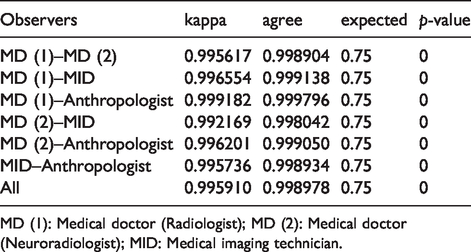
After obtaining the 16,000 classifications (100 exams, versus 10 case studies, in four different planes by four observers), we analysed those globally, per observer, and per plane. We have obtained global inter-observer agreement of 99.90%, with a kappa = 99.59%. These metrics were also compared for all observers pairwise (Table 2).
Global comparative view of paired observers’ agreement.
MD (1): Medical doctor (Radiologist); MD (2): Medical doctor (Neuroradiologist); MID: Medical imaging technician.
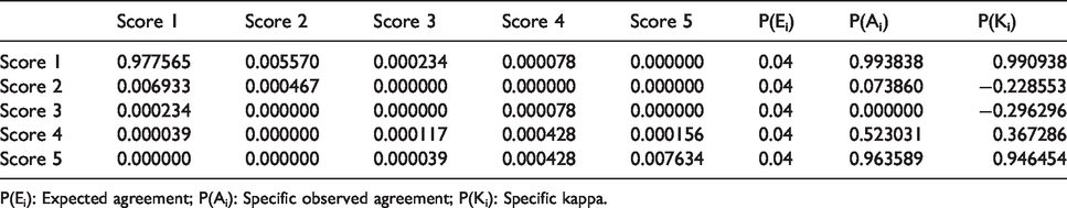
We can observe the discordance in scoring with a confusion matrix (Table 3). As Maclure and Willet 23 had pointed out, intermediate categories will often be more prone to misclassification, as can be perceived with the percentage of agreement (scores 2: 7.4%; scores 3: 0%; and scores 4: 52.3%). However, extreme categories of ordinal data were highly consistent (Scores 1: 99.4%; and 5: 96.4%), which indicates this problem could possibly be addressed in a binary sense.
Matrix of scores.
P(Ei): Expected agreement; P(Ai): Specific observed agreement; P(Ki): Specific kappa.
In this table, and analysing the specific observed agreement P(Ai), is evident that all images that were fully matched were almost always classified correctly (Likert 5) by the observers
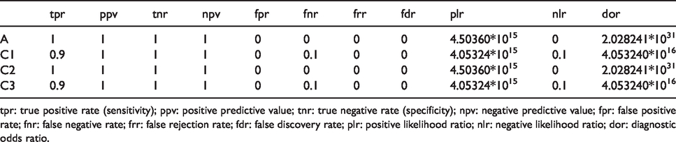
Looking at diagnostic metrics per slice, we noticed that the coronal 1 and coronal 3 performed slightly worse than the axial and coronal 2 view, which showed near perfect results (Table 4).
Diagnostics metrics per slice.
tpr: true positive rate (sensitivity); ppv: positive predictive value; tnr: true negative rate (specificity); npv: negative predictive value; fpr: false positive rate; fnr: false negative rate; frr: false rejection rate; fdr: false discovery rate; plr: positive likelihood ratio; nlr: negative likelihood ratio; dor: diagnostic odds ratio.
All observers detected perfectly all real-case individuals, thus academic background did not have any influence on the identification through matching of the inner ear anatomical features (Table 5).
Diagnostics metrics per observer.
tpr: true positive rate (sensitivity); ppv: positive predictive value; tnr: true negative rate (specificity); npv: negative predictive value; fpr: false positive rate; fnr: false negative rate; frr: false rejection rate; fdr: false discovery rate; plr: positive likelihood ratio; nlr: negative likelihood ratio; dor: diagnostic odds ratio.
As can be seen in Figures 6 and 7, which are compilations of nine images of the selected planes of different individuals, and which were used for the study, there are several differences in shape, size, relative orientation and relation of the structures between the diverse individuals, that permitted a correct classification by observers and the correct correspondence between the dataset and trial cases.
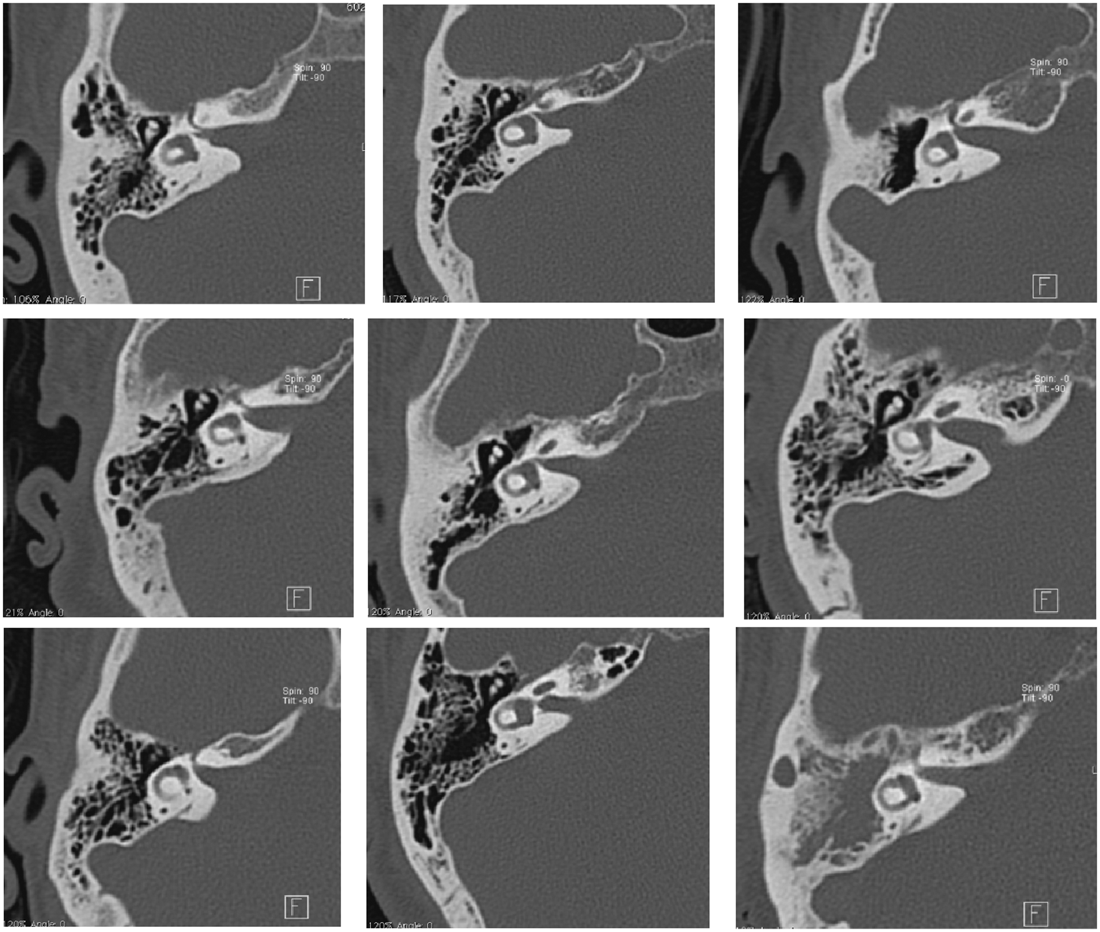
Example of the axial reference image in nine individuals of the sample, allowing observation of the various anatomical characteristics in the plane where the external semicircular channel is observed in all its extension.
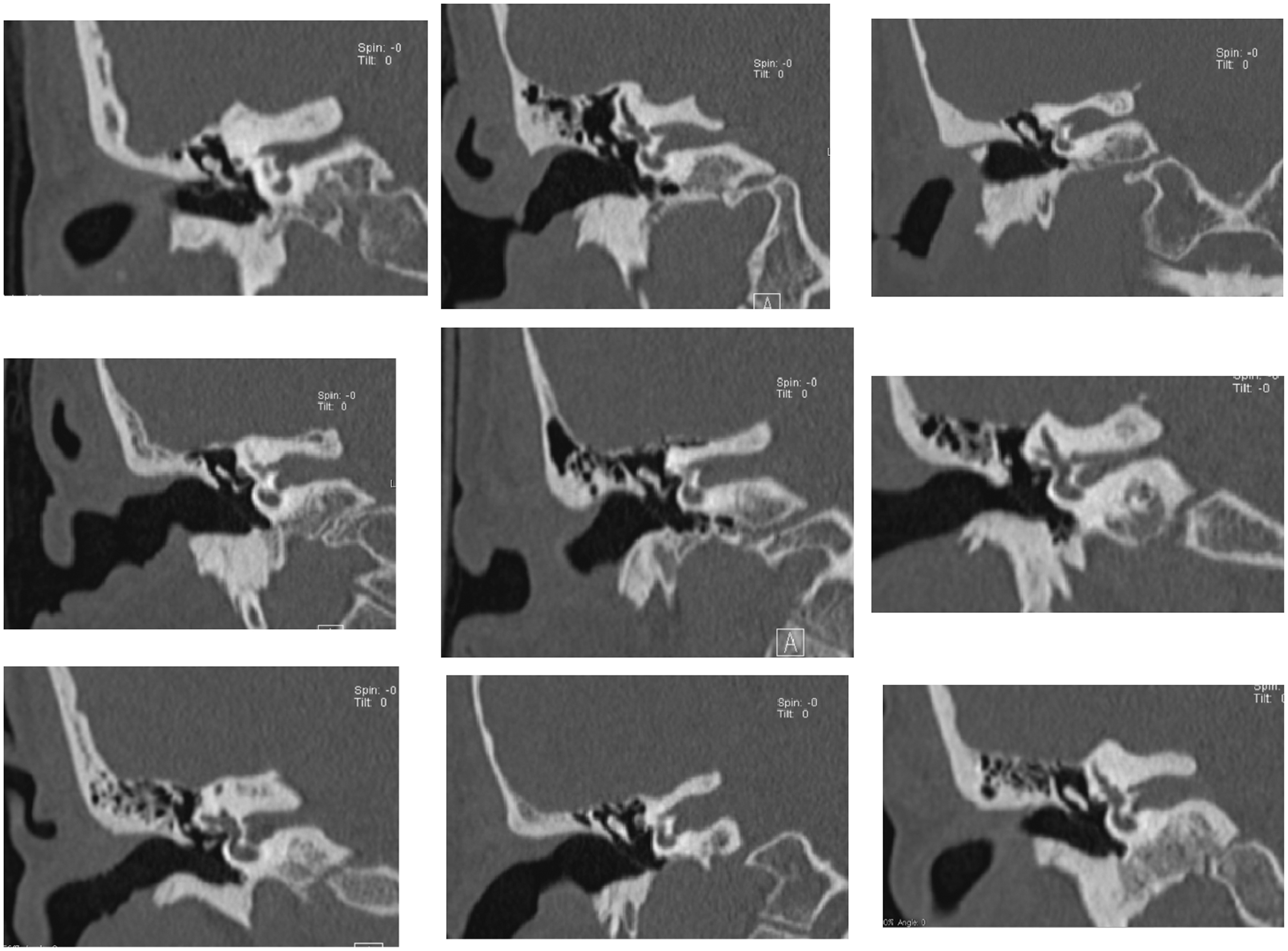
Example of the first coronal reference image in nine individuals of the sample, allowing observation of the various anatomical features in the plane where the fundus of the internal auditory canal, the crista falciformis and cochlear nerve foramen are observed.
Discussion
Although the usefulness of the internal structure of the temporal bone is already known in individual cases, its effectiveness was not, since it had not been proved by a statistical study that anatomic landmarks in this location are reliable enough to be accepted in court as a marker of individuality when evaluated by CT scans. In this context, we attempted to validate a concept present in the literature, but, at least to the authors’ knowledge, to date not validated by any observational study or with a statistical base.
In our work we found that all observers could perform a true positive identification or exclusion by comparing the problem images against the background images. They reached sensitivity and specificity of almost 100%, without false positive or false negative evaluations.
We also showed that previous expertise with CT images was not very important in the results. The radiologist, the neuroradiologist, the radiographer and the anthropologist obtained a 99.5% agreement in their observations, telling us that the learning curve to perform the matches would not be very difficult.
The images that performed better were the axial plane at the level of the lateral semicircular canal, and the coronal image where the apex and the first turn of the cochlea could be depicted.
The statistical analysis of Likert scores found that the problem could be addressed with a binary scale, since most of observations were highly consistent (scores 1: 99,4% and scores 5: 96,4%), which indicates that the problem could be solved in a simpler way, and has a match or non-match answer.
In summary, the statistics results confirmed our hypothesis, that differences in internal anatomic characteristics of the petrous bone are distinctive enough and could be perceived by observers, allowing matching or exclusion in an identification problem. This capability could be achieved in four reference images with precise anatomic landmarks, allowing this study to be reproduced by other investigators.
Thus, this basic research could in future be translated to real-case scenarios, where our conclusions could help to strengthen the identification process in a court trial. Basic research done in this setting will enable real-case scenarios to be examined from another perspective, and not as isolated single cases. The strength of a practical transfer to the field is supported by this study.
We are aware of some of the limitations of applicability inherent in this study. The first is due to the fact that ear exams represent a small part the of cranial exams realised. Thus, the total number of available exams for post-mortem tomographic comparison is reduced.
The second is concerned with our study design itself, since the evaluation was exclusively done using only the right temporal bone. This option was deliberate, in order to simplify the study, and to reduce the time taken and the complexity of the evaluation. However, we can confirm that during image selection, the authors observed that the structures analysed are highly asymmetrical. Therefore, the forensic matching should always be done with regard to the ipsilateral side.
Third, we are aware that we do not provide any direct comparison between ante-mortem exams and the respective cranium after skeletonisation, and that this is a major concern. This results from the fact that the lack of soft tissues might hamper observations, since the cranial soft tissues tend to mitigate radiation, which might alter the perception of the osseous details, thus interfering with the observer’s ability to perform the matching between structures ante and post mortem. The authors hope that this problem can be tested soon with a collection of skeletons. In any case, we argue that the procedure of the present study needed to be explored first, as it would not be worth trying this method further if it does not work in a basic research trial. Besides, we are confident that the changes in internal temporal anatomy and reference points will be minimal after skeletonisation, as we can see in identification processes based on the comparison of internal bone trabeculation between ante-mortem and post-mortem examinations.
We also believe that the differences resulting from the lack of soft tissues will have a small effect in images, because CT scanners have automatic dose modulation, compensating the absence of soft tissues.
We are further aware that even though the temporal bone is particularly resistant, in real-case scenarios with violent trauma, traumatic injuries may preclude attaining such accurate results. But it is also known that severe petrous bone destruction represents a minor subgroup of cases in forensic identification problems, since the causes of death are so diverse. Again, before proceeding for those cases, the accuracy of the approach in undamaged structures first has to be proven, which we did here.
Finally, we are aware that the values obtained for sensitivity and specificity in our study are very high, an aspect that requires confirmation by other study groups. The four observers knew in advance that there was one and only one correct correspondence, and that consequently all the remaining 99 hypotheses were incorrect, which could have conditioned the answers because there were no cases of null response. But as the reading was done blindly, without informing the observer about the quality of their answers, we hope that this has not influenced subsequent responses.
According to our bibliographic search there are no previous publications evaluating in an observational and statistical basis the performance of using temporal bone for human identification. There are only some isolated cases highlighted in the literature. In this context our work was inspired by previous papers using frontal sinuses, bone trabeculae, or dental characteristics for positive identification.
We selected an anatomic location with a lot of fine details and an image technique that clearly could depict these details. Ross et al. 25 previously published a study using anatomy landmarks in radiographs, which is a technique with fewer anatomic details than CT, and established the minimum number of concordant points needed to confirm positive identifications in X-rays. We went a little further and chose to use several landmarks in CT reference images, in order to obtain a global picture of confidence for identification.
As in the works of Ruder et al.10,24 and Quatrehomme et al., 14 we attempted to evaluate the capability of different observers to discriminate between osseous landmarks and use them for positive identification. Some authors use more or fewer observers in their studies, and have sometimes used assisted computer correspondence matching, but we feel that our methodology is in the scope of the published methods.
Some publications tried to evaluate the performance of readers with different kinds of expertise. In our results, the differences in achievement were not as high between observers as in other studies.10,24 Our outcomes were also a little higher in the scope of sensitivity, specificity and predictive values than previous studies.10,24 We think that these facts are related to comparing the same images in this ‘match trial’ and not the pre-mortem images with post-mortem images subjected to changes related to trauma or taphomonic factors. We also attribute these results to the great anatomical detail that could be depicted in this particular region using CT scans.
We hope that our work will lead forensic agents to consider CT of the temporal bone as a method worth trying in identification works, and that CT imaging is progressively integrated into forensic practice.
For the future, our biggest aim is to consider the applicability of this method in real identification scenarios, and conduct an experimental trial in which we can also undertake a similar methodological evaluation.
Conclusions
The multiple observer analysis of the anatomical features of the temporal bone by CT scanning is an imaging method that can contribute to human identification in the context of forensic problems. The study confirmed that the differences in internal anatomy of the temporal bone depicted by CT scans can be recognised with high confidence by several observers, meaning that they are capable of contributing to individual human identification.
In this study, the observers’ backgrounds did not significantly change the results. All were able to identify with all the blind cases against the total sample with confidence. Statistical analysis reinforces the view that anthropologists or radiology technicians can perform as well as a radiologist. Sensitivity and specificity values were equal for all observers.
It should be noted that in over 4000 classifications that each observer has done, there was not a single false positive. The lack of false positives in the experiment is extremely important, as it shows that the method can avoid the errors associated with incorrect and presumptive identification, which entail costs while leading the identification the wrong way. The absence of false negatives is also relevant, confirming temporal bone CT is a reliable screening method (when available), before proceeding to more expensive confirmatory studies such as genetic analysis.
Footnotes
Declaration of conflicting interests
The authors declared no potential conflicts of interest with respect to the research, authorship, and/or publication of this article.
Funding
The authors received no financial support for the research, authorship, and/or publication of this article.
“All authors have completed the ICMJE uniform disclosure form at ![]() and declare: no support from any organisation for the submitted work; no financial relationships with any organisations that might have an interest in the submitted work in the previous three years; no other relationships or activities that could appear to have influenced the submitted work.”
and declare: no support from any organisation for the submitted work; no financial relationships with any organisations that might have an interest in the submitted work in the previous three years; no other relationships or activities that could appear to have influenced the submitted work.”