Has the Instability of Personal Incomes been Increasing?

Abstract

This paper examines trends in the instability of personal incomes in Britain in terms of changes in the transitory variance and in volatility, measures that have received much recent attention in research about the USA. It is shown that, although US measures have trended upwards over the past two decades, there is no such trend in Britain between the early-1990s and the mid-2000s. Explanations for these differences are discussed.

Keywords

Transitory variance income volatility income instability British Household Panel Survey longitudinal data

1. Introduction

Income inequality is most commonly examined from a cross-sectional perspective — the questions are how much inequality is there in a given year and what are the trends over time? But economists have also long been interested in inequality from a longitudinal perspective, examining the longitudinal variability of personal incomes over time, and the extent to which the crosssectional dispersion of income represents differences between individuals that are long-lasting (‘permanent’) or transitory — a variance components approach that dates back to at least Milton Friedman. The greater the transitory variance, the more income risk there is, broadly speaking. In this paper, I provide new evidence about trends in the instability of personal incomes in Britain using data covering the period 1991 through 2006, drawing on research undertaken for my recentlypublished book (Jenkins, 2011).

Fluctuating incomes are undesirable because most people prefer greater stability in income flows to less, other things being equal, if only because stability facilitates easier and better planning for the future. But, more than this, by definition, transitory income variation is an idiosyncratic shock which cannot be predicted at the individual level; greater transitory variation corresponds to greater income risk, and this is undesirable. How undesirable it is depends on the extent to which individuals are insured against such risks. In this assessment, it is important to distinguish between transitory variation in an individual's labour earnings and transitory variation in a more comprehensive measure of economic well-being such as household net income adjusted for differences in household size and composition (‘equivalised’). Insurance against labour income risk is provided by social insurance against income loss due to unemployment, ill-health, and retirement (combined with social assistance), and by public and private schemes covering income loss through accidental injury or sickness. Individuals may also self-insure by accumulating stocks of assets that can be drawn on in bad times (or postponing purchases of new ones), by adjusting their labour supply, or by income sharing within families (for example a spouse might work more hours if her partner is laid off). A comprehensive household income measure is intended to include income from sources other than labour earnings, and income accrues to all persons in the population (whereas earnings only go to individuals in paid work). Thus transitory variation in measures of household income is more plausibly associated with income risk that is of social consequence than transitory variation in the labour earnings of an individual.

The argument that the transitory variance is a good measure of income risk needs to be tempered because household income outcomes (as well as labour income outcomes) partially reflect choices made voluntarily and are hence of less social concern. Income falls arising from choosing to work shorter hours are less socially worrisome than falls arising from lay-offs associated with firm closures, and it is moot whether changes in income associated with changes in household composition such as family formation or dissolution or the birth of a child should be treated as wholly voluntary. For a model-based approach to identifying earnings uncertainty, see Cunha, Heckman, and Navarro (2005).

Because it is difficult to distinguish variations arising from these types of income change from variations arising from involuntary and unpredictable sources, and also because there are practical problems with estimating transitory income variation (see below), changes in transitory variation over time are imperfect measures of changes in income risk. For this reason, there is a growing US literature which supplements estimates of transitory variation trends with estimates of trends in income ‘volatility’. The different approaches are reviewed by Moffitt and Gottschalk (2008b) and Shin and Solon (2011).

This paper examines trends in both the transitory variation and volatility of income in Britain. Most empirical studies have analysed men's employment earnings rather than household income. I present estimates using both types of income variable in order to check whether the conclusions drawn are sensitive to this choice and also to facilitate some cross-national comparisons, especially with the USA, a country where this topic is receiving substantial attention. I show that the instability of personal incomes has changed little in Britain over the period between the start of the 1990s and the mid-2000s, and consider explanations for this finding. For analysis of trends in income mobility defined differently, see Jenkins (2011, Chapter 5).

The analysis is based on waves 1–16 (survey years 1991–2006) of the British Household Panel Survey (BHPS), using data for individuals belonging to the original sample that began in 1991. The principal measure of income used for individuals is their real net household income, equivalised using the modified-OECD equivalence scale and expressed in pounds per week (January 2008 prices) pro rata. Net household income includes employment and self-employment earnings, income from cash benefits, tax credits and the state retirement pension, income from financial assets including occupational and private pensions, and private transfer income, from which are deducted income tax, national insurance and local tax payments. The definitions of income, equivalence scale, and price deflator, are the same as used in Britain's official personal income distribution series: see Department for Work and Pensions (2011). For further details of the sample and the BHPS income measure, see Jenkins (2011, Chapters 2 and 4). To facilitate comparisons with other research, I also use a measure of gross household income, which is the same as net household income except that income tax, national insurance and local tax payments have not been deducted. I also consider the instability of real monthly labour earnings for male employees aged between 25 and 55 years. Gross household income and earnings measures are also expressed in January 2008 prices.

All calculations have been undertaken using data that are weighted, in order to address potential issues of nonresponse including attrition. Distributions are trimmed to inoculate estimates against the adverse effects of outlier income values and changes; the bottom 1 per cent and the top 1 per cent of observations are dropped prior to the calculation of all longitudinal measures. This is common practice in research on this topic: see for example Gottschalk and Moffitt (2009) and references therein.

2. Estimation of the transitory variance and of volatility

The transitory variance has been estimated using both model-based and non-model-based methods.

Variance components model-based estimation of the transitory variance

There is a long tradition of fitting econometric models to specifications that go beyond the simplest variance components model. Applications to men's earnings include Abowd and Card (1989), Baker (1997), Baker and Solon (2003), Chamberlain and Hirano (1999), Haider (2001), Guvenen (2009), Hause (1980), Lillard and Willis (1978), Lillard and Weiss (1979), MaCurdy (1982), Meghir and Pistaferri (2004), and Moffitt and Gottschalk (2002, 2008a, 2008b, 2011 [originally 1995]). All this research fits models to US or Canadian data. Applications to British men's earnings data are Dickens (2000), Kalwij and Alessie (2007), and Ramos (2003). Daly and Valletta (2008) compare earnings dynamics in Britain, Germany, and the USA. An excellent review of variance components modelling and recent extensions is provided by Meghir and Pistaferri (2010). There have been few applications to broader measures of household income; notable exceptions are Biewen (2005) for Germany, and Duncan (1983) and Stevens (1999) for the USA. The only studies applying these methods to British data on household income that I am aware of are Blundell and Etheridge (2010) and Devicienti (2011).

Although variance components models have advantages for estimating transitory variances and their trends because of their sophisticated specifications to account for the complexities of income dynamics, they also have their weaknesses. These have been stated trenchantly by Shin and Solon, who write that ‘the parametric models used … are arbitrary mechanical constructs and the resulting estimates of trends can be sensitive to arbitrary variations in model specification’ (2011, p. 4). To illustrate this point, they refer to Baker and Solon (2003) who fit general models to Canadian tax record data on men's earnings. The large sample facilitates more thorough specification checking than is possible with the smaller US data sets used in most previous studies. Shin and Solon report that Baker and Solon (2003) ‘strongly rejected the restrictions of Moffitt and Gottschalk's (1995, 2002) preferred model and found that imposing those restrictions substantially biased the estimation of Canadian trends in components of earnings variation’ (2011, p. 975). Guvenen (2009) also draws attention to the difficulties of differentiating between different specifications from the panel data sets on earnings that are typically available.

Non-model-based estimation of the transitory variance and of volatility

Given these issues, simpler methods of estimating the transitory variance and volatility remain popular. The most commonly-used non-model-based estimator of the transitory variances is that of Gottschalk and Moffitt (1994, 2009) and Moffitt and Gottschalk (2008b), which has also been used by Bartels and Bönke (2010), Beach, Finnie, and Gray (2010), Gosselin (2008), Gosselin and Zimmerman (2008), and Keys (2008). I label this method ‘MG2’ to distinguish it from the simpler (‘MG1’) estimation method used by Moffitt and Gottschalk (2002), Hacker (2008), and Hacker and Jacobs (2008).

The MG2 method works by first calculating the longitudinal average of each person's log income over a time window of fixed width, say T years. This provides an estimate of the person's ‘permanent’ income for that period. The transitory incomes for each individual within the window are derived as a difference between this permanent income and observed log income, from which can be calculated the individual-specific transitory variance. The overall sample transitory variance is the average of these variances. The sample permanent variance for each window is calculated from the differences between each person's permanent income and the sample grand mean of these, with an adjustment to account for the fact that the mean contains a proportion of the transitory component that has not been fully averaged to zero over the T year window. See Gottschalk and Moffitt (2009: 7) for full details of the formulae characterising the MG2 method. Repetition of the calculations over a set of moving windows provides estimates of variance trends.

Without fitting sophisticated variance components models — which brings its own problems, as discussed above — it is inevitable that measures derived using methods like MG1 and MG2 reflect the variability from permanent shocks not from only transitory ones. Shin and Solon (2011) argue that this is a virtue of such measures on the grounds that permanent shocks are even more consequential as transitory ones. Their own calculations are based on a third measure, ‘volatility’, which has also been used by researchers including Dahl, DeLeire, and Schwabish (2007), and Dynan, Elmendorf, and Sichel (2008), and Dynarski and Gruber (1997).

Volatility in a given year is measured by the sample standard deviation of the distribution of individual changes in log income between that year and an earlier year. Changes are typically measured over a one- or two-year horizon.

3. Trends in the transitory variance and volatility of income

I present BHPS-based estimates of the transitory variance and volatility, and compare them with other estimates for Britain and the USA where possible. Following common practice, all the estimates presented are based on income variables adjusted in advance to remove the systematic variation of income with age. The idea is that such variation is predictable and hence less relevant to the concept of mobility as income risk. Thus, for each sample, income is first regressed on a fourth-order polynomial in age, and the analysis is of the residuals from the fitted equation. Analysis of unadjusted incomes led to very similar conclusions. Estimates of the transitory variance are based on balanced samples of individuals with valid incomes for each year of a seven-year moving window, with sevenyear averaging. The sample sizes for household income calculations are around 4,000 persons from about 2,000 households for each window's sample. Repetition of the calculations using five-year windows does not change the conclusions.

The transitory variance of net household income

Estimates derived from income data for all individuals are presented in figure 1. It is clear that there has been no increase in the transitory variance of income in Britain between the mid-1990s and the mid-2000s. A downward trend is perceptible for the period as a whole and this is consistent with US findings that the transitory variance changes counter-cyclically (Moffitt and Gottschalk 2008b; Shin and Solon 2011). Unemployment rates in Britain were falling throughout the period. Successive estimates are similar but the decline from the beginning of the observation period to the end is from 0.048 to 0.040, a decrease of 17 per cent. Correspondingly, the fraction of the total variance that is transitory fell from around 37 per cent through the 1990s to 33 per cent by 2003. With an approximate standard error of around 0.001 for each MG2 variance estimate, year-on-year changes are not statistically significant, but the change between the mid-1990s and the mid-2000s as a whole is.

Figure 1.

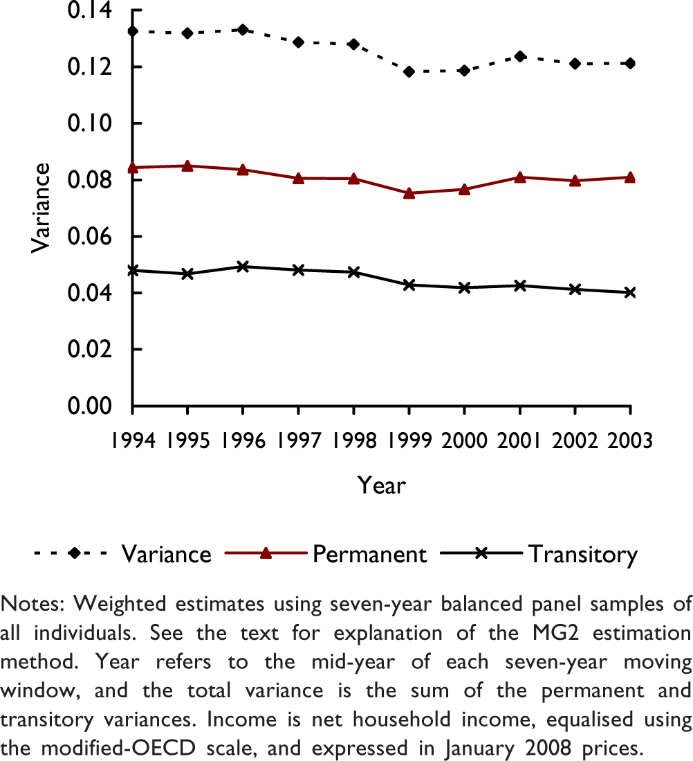
Transitory and permanent variances of log net household income, by year

There are few estimates for Britain to compare these with. Perhaps the closest are those of Devicienti (2011) who fitted several variance component model specifications to BHPS data for 1991–8 using the same income definition as mine. There is consistency in our estimates in the sense that Devicienti finds little change in the variance loading factors over the period. Blundell and Etheridge (2010) fitted a variance component model to the net household incomes of a sample of household heads aged 25–60. Among household heads with positive labour earnings, their model parameters imply that the transitory variance was relatively constant from 1991 through to 2003. However when they also include household heads without labour income in their sample, the predicted transitory variance is slightly U-shaped over the same period. It is unclear whether this trend differs from the ones shown in figure 1 because of the different modelling approaches used (variance component models versus MG1 and MG2 estimators) or different sample selections. To investigate the latter aspect and to facilitate further comparisons with other studies, I recalculate MG2 estimates using different income definitions and subgroups.

An advantage of a gross income measure is that it allows closer comparisons with recent estimates for the USA based on gross income measures derived from the Panel Study of Income Dynamics (PSID). When I apply the MG2 method to data for (equivalised) gross household income, but using the same samples and also ageadjusted in the same way as for net income, I derive the same conclusions about trends — a slight fall over the period as a whole (results not shown). The main difference is that the estimates for each year of the transitory variance are slightly larger, by almost 2 percentage points. The larger estimates for gross income are to be expected; one of the roles of the tax system is to smooth out the consequences of adverse income shocks, and the gross income measure does not pick up this aspect (since it is a pre-tax measure). The difference in estimates is not larger, however, because much of the income smoothing work is done by social security benefits rather than the tax system.

For the USA, Gottschalk and Moffitt (2009) report MG2-based estimates of the transitory variance for ‘log annual family income’, using nine-year moving windows covering the beginning of the 1970s through to around 2000. The family income definition is similar to the BHPS gross income definition in that it is also a ‘pretax post-transfer’ definition (to use the US phrase), and both are equivalised (Gottschalk and Moffitt use the US official poverty line). The main difference is that income from the principal US in-work benefit, the Earned Income Tax Credit (EITC), is not included in the PSID income definition, and nor are receipts from in-kind benefits of which the most important is Food Stamps (now called Supplemental Nutrition Assistance Program). Income from tax credits is included in the BHPS definition and there is no British counterpart to Food Stamps.

Gottschalk and Moffitt (2009, Figure 5) report estimates of the transitory variance that increased over the 1990s, continuing a secular rise that had been in progress for the previous two decades. Although the rise was not continuous, it was marked, with the estimated transitory variance going from below 0.120 in 1994 to above 0.140 in 2000, which is a rise of at least 16 per cent. Gosselin and Zimmerman (2008) also use PSID data to estimate trends in the transitory variance using MG2 methods with six-year moving windows and find, by contrast with Gottschalk and Moffitt (2009), that the transitory variance rose over the first half of the 1990s but did not increase further in the second half of the 1990s (Figures 5 and A1). Some of the differences may arise because Gottschalk and Moffitt (2009) consider all individuals in families whereas Gosselin and Zimmerman focus on adults aged 25–64, and it may be that the variability of circumstances for young adults and old people has increased.

It is not only the upward trend for the US transitory variance that differs from the British experience, but also the magnitude of the variance itself. Gottschalk and Moffitt's US estimates are roughly twice as large as the estimates for Britain reported above. This differential is likely to be an over-estimate because of the exclusion of EITC income and Food Stamps from the PSID definition of family income — one would expect these sources to have a stabilising impact. But, all in all, the comparison suggests that income risk is substantially larger for US families than for British ones.

It is of interest to explore the differences between subgroups not only for their intrinsic interest, but also to see whether this may account for some of the differences in findings. Figure 2 shows estimates of the transitory variance in gross household income for each of seven person types differentiated by age and sex. The corresponding chart for net household income is very similar and not shown for brevity. The trend downwards in the overall transitory variance is driven by the downward trend for the most numerous groups, that is, men and women aged 30–59 and dependent children. The variances for these three groups are similar, which is unsurprising as they are mostly couples with children sharing a household. Men and women aged 60 years or more have substantially lower transitory variances than the other groups (though they have a downward trend as well) and the transitory variance is also a smaller fraction of the total variance. The vast majority of people of this age have retired from the labour market and state, occupational, or private pensions are the main sources of income, most of which are relatively fixed. (This is before the financial crisis at the end of 2008 when interest rates fell substantially.) Also consistent with expectations, the groups with the largest transitory variances of gross household income are adult men and women aged below 30, that is, those likely to have the highest rates of movement between paid work, education and non-employment, and also making transitions between their parents' household and their own (which affects their total household income and the equivalence scale).

Figure 2.

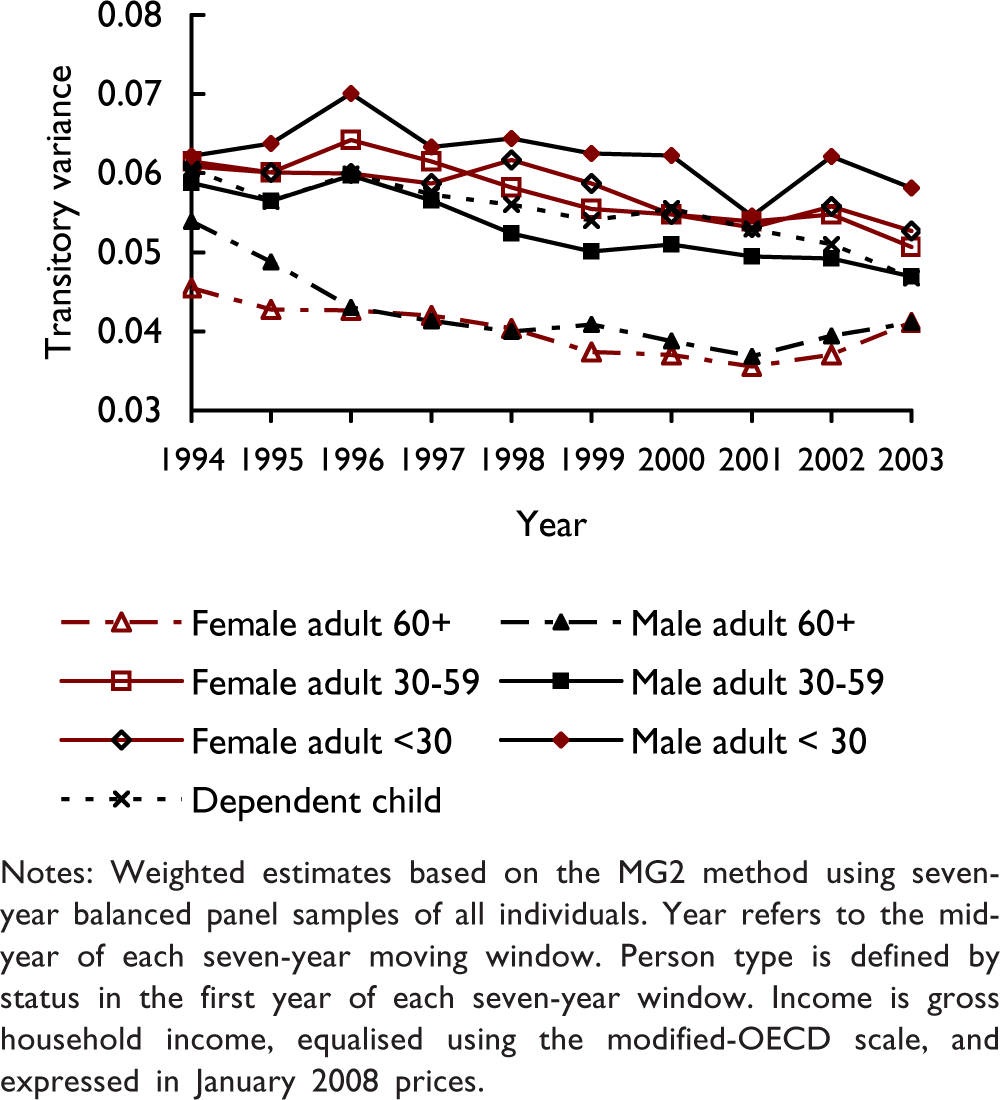
Transitory variance (log gross household income), by person type and year

The transitory variance of employment earnings for prime-aged male employees

Now consider estimates of the transitory variance of labour earnings for prime-aged male employees. This is what has been studied most in research on income instability and so there are more possibilities for comparisons of findings. Also, since men's employment earnings form the largest share of household income for households of working age on average, transitorypermanent variance patterns for individual earnings and household income may be informative about the factors underlying the patterns for household income. The variance decomposition is shown in figure 3. (There are about 700 men in the sample for each seven-year window.) The estimates suggest that the transitory variance remained constant between the mid-1990s and mid-2000s, though the overall variance increased.

Figure 3.

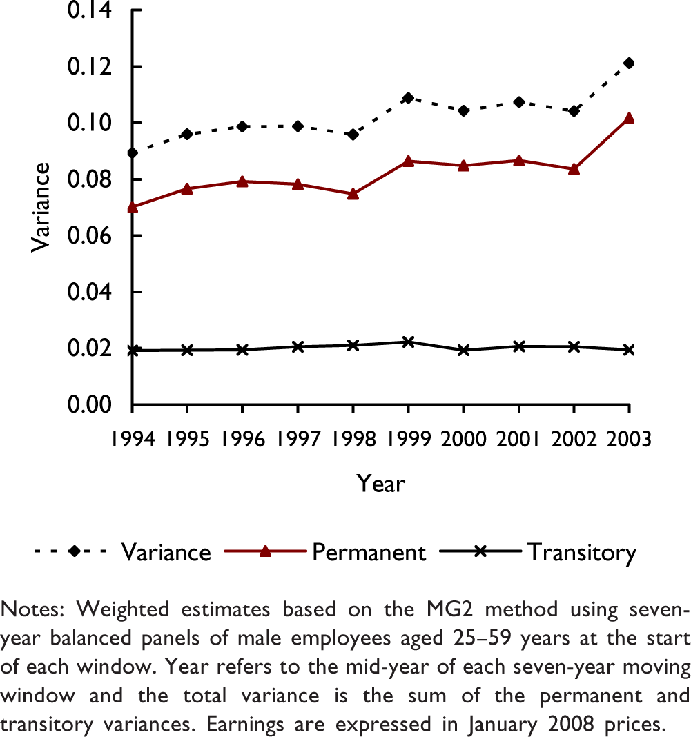
Transitory and permanent variances of log gross earnings for prime-aged male employees, by year

At first glance, my finding of no overall trend in the transitory variance of men's earnings conflicts with that of Dickens (2000), who used large samples from administrative records on earnings for British male employees aged 22–59 years covering the period 1970–1995. (For estimates covering 1975–2001, see Kalwij and Alessie, 2007.) On the basis of variance component model estimates, Dickens finds that both the transitory and permanent variances increased over the period for most birth cohorts. One explanation for the different findings concerns the coverage of the data sets. Dickens used the New Earnings Survey panel, and this does not include pay information for individuals with earnings below the income tax threshold (and hence without a PAYE record). There is no such restriction in the BHPS and it was for permanently-low-paid workers that I find a small downward trend in the transitory variance in the late 1990s. (See Jenkins, 2011, for details.) A related point concerns the groups of earners for whom transitory variances are calculated. My BHPS analysis refers to men who have positive earnings at each of seven consecutive annual interviews (a balanced panel), whereas Dickens and many other modellers use unbalanced panels. However, it is unclear that such compositional changes would be responsible for an increase in the transitory variance over a period when unemployment rates were falling and jobs likely to be more stable rather than less. Moreover, when I repeated the calculations using an unbalanced panel (only requiring positive earnings for at least two years within each seven year window), I find that trends are the same as pictured in figure 3. The only change is a reduction in the estimated variances for each year.

Another potential explanation for the differences between Dickens' results and mine is that the specific periods covered differ — my estimates refer to a period beginning in the mid-1990s, which is when his sample ended. To be convincing, this argument requires additional evidence that the transitory variance stopped rising in the late 1990s. The studies by Ramos (2003) and Daly and Valetta (2008) are relevant to this. Both fitted variance components models to BHPS data on men's employment earnings, for the period 1991–9 and 1991–8 respectively. Both papers suggest that the transitory variance fluctuated over the period, though on a slightly rising trend for several birth cohorts according to Ramos (2003, Figure 3).

On the one hand, these results might be interpreted as suggesting that the MG2 method provides biased estimates. On the other hand, there is the earlier argument that estimates of trends from variance components models may be sensitive to the choice of specific model specification. For example, despite only relatively minor differences in model specification, the estimated time path of the transitory variance is quite different in the Ramos (2003) and Daly and Valetta (2008) studies. This sensitivity is one of the arguments for also examining estimates of volatility. Before doing so, I compare the British estimates of the transitory variance with those of other countries.

The leading estimates of the transitory variance in US men's earnings are those of Gottschalk and Moffitt (1994, 2009) and Moffitt and Gottschalk (1995, 2002, 2008a, 2008b) derived using both MG2- and variance components model-based methods. As in research by others using PSID data, they find that the transitory variance for men's earnings rose over the 1970s and 1980s, but then stopped growing around 1990. From then until 2003 — the period for which there are BHPS estimates — the transitory variance fell slightly and then rose again at the end of the period: see for example Gottschalk and Moffitt (2009, Figure 1). Moffitt and Gottschalk (2008a) report the same trend between 1991 and 2003 using administrative record data rather than PSID data as in the other studies. The authors conclude that ‘the transitory variance did not show a trend net of cycle over this period’ (2008a, i) and draw attention also to the close association between changes in the transitory variance and changes in the unemployment rate.

The US findings throw up several contrasts with those for Britain. There are differences in substantive findings. The U-shaped trend in the US transitory variance over the 1990s is not suggested by my estimates or any of the other British studies cited earlier. However, the US result about trends is largely accounted for by cyclical factors. If these work in the same way in Britain, then the steady decline in the unemployment rate in Britain over the fifteen years starting in 1993 is an explanation of why the transitory variance did not increase in the decade from the mid-1990s. Second, the transitory variance for men's earnings is smaller in Britain than in the USA. For instance, around 2000, I estimate the British figure to be 0.02, compared to the corresponding US estimate, 0.14 (Gottschalk and Moffitt, 2009, Figure 1). Some of the differences in levels may reflect transatlantic differences in flexibility of labour market adjustment (Jenkins, 2011).

Income volatility

I now consider estimates of volatility in household income among all individuals and in earnings for primeaged male employees: see figure 4. Incomes are ageadjusted, as before, but the adjustment makes virtually no difference to the estimates derived. One advantage of taking two distributions just one year apart is that potential selectivity issues associated with requiring survey participation over longer periods (as with the MG2 method) are minimised.

Figure 4.

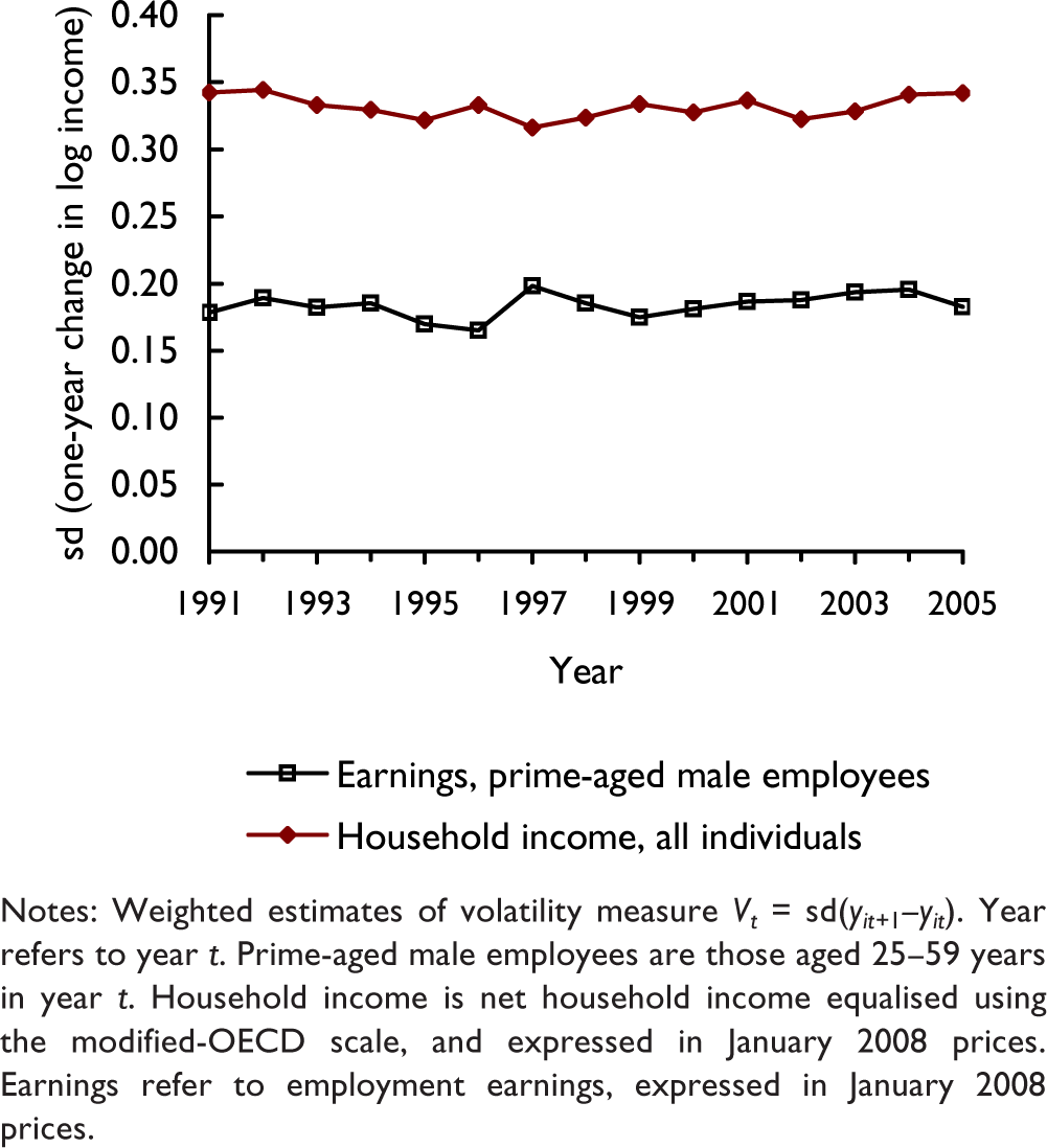
Volatility of household income (all individuals) and of earnings (prime-aged male employees), by year

The estimated trends in volatility are similar to those for the transitory variance. Variability is greater for household income among all individuals than for earnings among prime-age male employees according to both types of measure. In addition, there is no clear trend upwards or downwards over the period as a whole. There are fluctuations from one year to the next but they generally lie within the bounds of sampling variability (the standard error for each measure in a given year is about 0.01). Calculations of volatility in household income for subgroups (not shown) reveal that volatility is greatest for adults aged less than 30 years compared to other age groups. Excluding individuals with selfemployment income or with imputed gross income components does not change the picture concerning trends either.

All other estimates of volatility that I am aware of refer to the USA. There is only one paper that has considered the volatility of household income: Dynan, Elmendorf, and Sichel (2008) report estimates for a family income measure that is not equivalised. Their samples are rather specific, being restricted to individuals who are household heads aged 25 or more and not retired and who remain the head of their household in the two distributions compared (these are two years apart to reflect the PSID's biannual interviewing from 1997). For this group, Dynan, Elmendorf, and Sichel report a discontinuous rise in income volatility between 1990 and 2004, with most of the rise in the first five years of the period (2008, Figure 3). This follows a steady rise in volatility over the 1970s and 1980s. For the volatility of the earnings of household heads (mostly men), there are similarities and differences. Dynan, Elmendorf, and Sichel (2008, Figure 1) estimates imply a rise in volatility over the thirty year period, but changes are more discontinuous than for household income. In particular, earnings volatility is estimated to rise at the start of the 1990s, fall back, and then rise again at the start of the 2000s. Some of the fine detail in the year-onyear changes may be obscured because Dynan, Elmendorf, and Sichel (2008) smooth the series they present, showing three-year moving averages. In any case, the US volatility estimates for the early 2000s are markedly higher than those for Britain: between 0.45 and 0.50 compared with around 0.35, respectively.

For US earnings volatility trends, the leading paper is by Shin and Solon (2011), also using PSID data. Shin and Solon find that earnings volatility rose over the fifteen years after the turn of the 1970s, and declined over the next five years. Over the first half of the 1990s, volatility was flat or fell slightly, but then from the mid-1990s started to rise again through to 2004. At this time, earnings volatility was around 0.5, which is substantially larger than the British estimate of around 0.2 shown in figure 3. Rather than pointing to any secular trends in volatility, Shin and Solon emphasise that earnings volatility is highly correlated with the US civilian unemployment rate (2009, Figure 1). This point echoes Moffitt and Gottschalk's (2008a, 2008b) finding that there is a close association between the transitory variance and the unemployment rate.

4. Explaining transatlantic differences in levels and trends

What explains the transatlantic differences in the levels of and trends in household income instability? Britain's lower transitory variance and volatility compared to the USA is straightforwardly explained by the differences in the comprehensiveness and generosity of their welfare states. (For a comprehensive comparison of these, see Walker, 2005.) For people of working age in Britain without a job, there are means-tested social assistance benefits that are universally available and available indefinitely (subject to work availability conditions) and supplementing social insurance unemployment benefits that have increasingly low coverage. These include means-tested assistance with high housing costs. The gap between the total income that the average person can get when working and the total income gained if not working has increased in Britain over the past two decades, especially with the introduction of tax credits for low income working families (reflecting the Labour government's goal to ‘make work pay’). Nonetheless, the decrease in household income that is associated with losing a job is substantially greater on average in the USA than in Britain. See Jenkins (2011) for further discussion.

Although differences between Britain and the USA in levels of household income risk are plausibly explained by differences in their welfare states, what explains the differences in the trends? In particular, why was there no significant change over the 1990s in Britain? Arguably, differences in trends can be explained partly by the differences in the economic cycle (see above) and, again, partly by differences in welfare states. Regarding the latter, the case is that, not only does Britain provide a more comprehensive and universal social safety net than the USA, but its safety net is better able than the US one to cope with change and continue to offset the impact of adverse income shocks on families and individuals. This argument is plausible but needs verification. Another argument is simply that the USA is an exceptional case: see the extensive discussion of the growing privatisation of risk in the USA by Gosselin (2008) and Hacker (2004, 2008), a phenomenon which does not appear to have a British counterpart. Again, this argument has plausibility. Nonetheless, it remains surprising that no significant changes in income instability are apparent in Britain during the 1990s (for either gross or net household income), when there were major changes to the tax-benefit system introduced by the Labour government from the late 1990s onwards. Macroeconomic cycle impacts aside, if the nature of the welfare state changed, should this not have had impacts on income stability and not only on cross-sectional features of the income distribution such as poverty rates? I hypothesise that these points can be reconciled if one acknowledges that there was change over the period, but various underlying factors had offsetting influences.

Offsetting influences?

I examine this hypothesis by looking at trends in the transitory variances of income components. (See Jenkins, 2011, for additional analysis of changes in the contribution of different income sources to longitudinal variability over a period in income itself.) Total income is broken down into the five types: labour income (from employment or self-employment) of the household head, labour income of the spouse (if present), benefits and tax credits (including the state retirement pension), other income such as receipts from investments and savings, and private transfers, and deductions of income tax, employee National Insurance Contributions and local taxes. The analysis method is the same as used for the USA by Gottschalk and Moffitt (2009, Figure 6). Transitory variances are computed for each source using the MG2 method, as before, except that incomes values are used rather than log incomes given that families may genuinely have zero income from several income sources. Incomes are expressed in January 2008 prices but not equivalised. Deductions from income are treated as positive values for this exercise. Following Gottschalk and Moffitt, I express estimates for each source relative to their value in the initial year (1994). Figure 5 shows the results. These refer to samples of individuals aged 25–55 years in the first year of each seven-year window.

Figure 5.

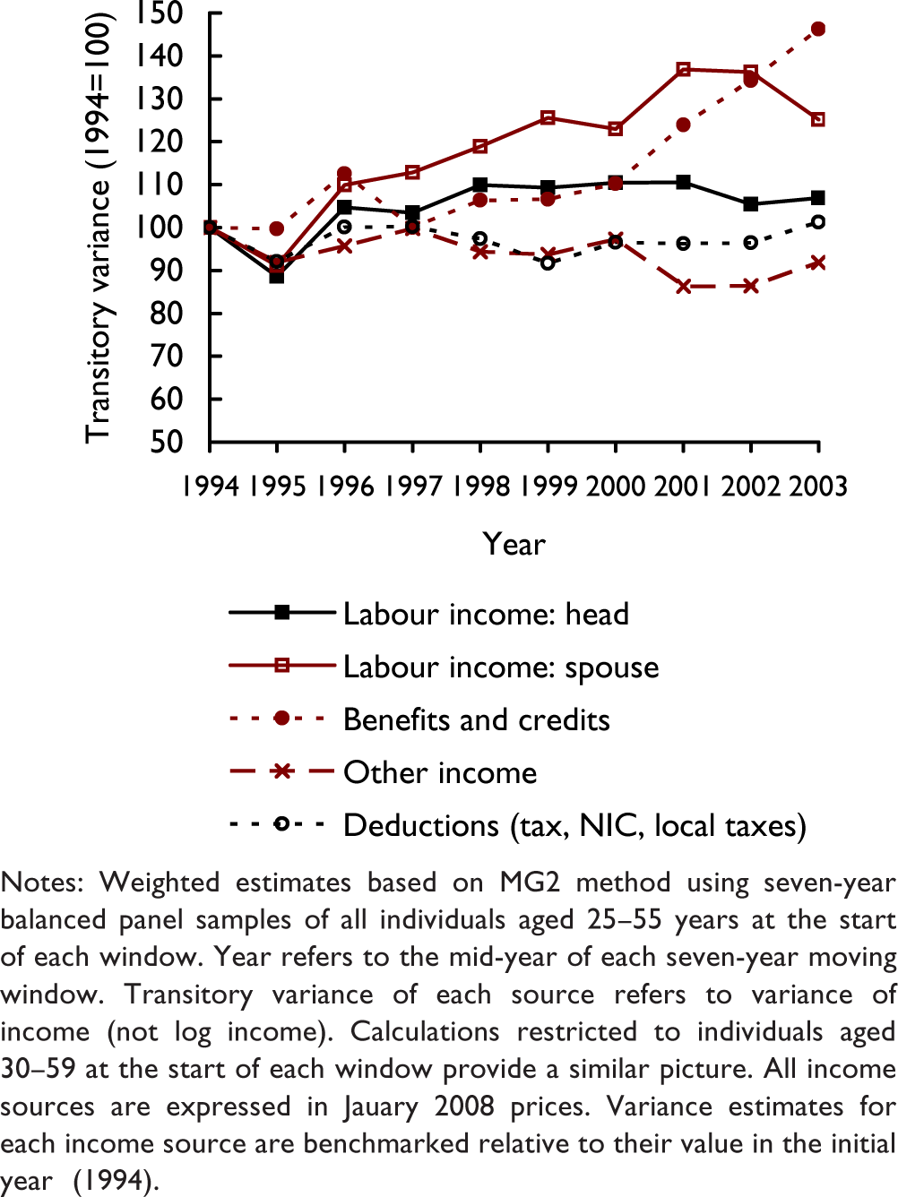
Trend in transitory variances of income sources

There is some evidence of offsetting forces in action; some transitory variances increased over time and some decreased. Increases over time are apparent for spouse's labour income throughout the period, and for benefits and credits from around 1999 onwards. It is tempting to link the former with the secular increase in women's labour force participation, which was perhaps also accompanied by instability in job holding. It is also tempting to link the trend in the transitory variance for benefits with the introduction of Working Families Tax Credit in 1999. Job instability of the sort just mentioned could also have knock-on consequences for tax credit eligibility and, in addition, income instability may arise from imperfect administration of the tax credits programme. (On this, see House of Commons Treasury Committee, 2006.) Otherwise, I note that the transitory variance for the principal income source for households of working age, head's labour earnings, has a relatively flat trend over the period (which is consistent with the results for log earnings shown earlier), and is most likely the principal driver of the relatively flat trend in the transitory variance for total income. A complete decomposition would also need to examine changes in correlations across transitory components, and changes in the shares of each source in total income. Repeating the analysis using all individuals (estimates not shown) leads to a picture about trends that differed in only two respects. One is that the transitory variance for benefits was closer to its 1994 value throughout the 1990s (but then also increased), and the other is that the transitory variance for ‘other’ income decreased below its 1994 value from the end of the 1990s, and it is unclear what is behind this.

The results for Britain echo those for the USA reported by Gottschalk and Moffitt (2009, Figure 6), as they also report an upward trend in the transitory variance for benefits (‘transfer income of head and spouse’ which is largely income from welfare programmes), though it was also accompanied by a rise in the transitory variance of ‘other nonlabor income of head and spouse’. Gottschalk and Moffitt conjecture that the results for benefits may have resulted from the welfare reforms which began in the early 1990s, and which led to higher welfare exit rates and shorter welfare spells.

In sum, although the aggregate picture for Britain is one of little change in income instability over the decade and a half since 1990, this does not mean that the underlying structures of income dynamics necessarily remained constant too. The decompositions by income source suggest that there were various influences at play over the period and with offsetting roles.

5. Concluding remarks

There is substantial scope for further research on the topic of income instability, much of which awaits further longitudinal data not only for Britain but also for other countries. For instance, past experience suggests that the major recession that began at the end of 2007 will be associated with an increase in income instability, and this needs to be investigated. Also, it is too early to judge conclusively how differences in welfare states between countries are associated with differences in income ‘risk’. The quotation marks are a reminder that the evidence about this presented here, and in other studies, is indirect — based on observations of longitudinal variability in incomes ex post.

Further research is needed on the connections between income mobility, risk, and economic insecurity, taking account of the extent to which families can transfer resources across time and their ability to insure against adverse shocks. In addition, there remain unresolved debates about the relative merits of measures of volatility and transitory variance for examining income instability (see Gottshalk and Moffitt, 2008b, and Shin and Solon, 2011). And how should measures of income instability over time enter into social assessments along with concerns about inequality, and changes in the dispersion of ‘permanent’ income differences between individuals in particular?

References

Abowd

Card

(1989), ‘On the covariance structure of earnings and hours changes’, Econometrica, 57, pp. 411–45.

Baker

(1997), ‘Growth-rate heterogeneity and the covariance structure of life-cycle earnings’, Journal of Labor Economics, 15, pp. 338–75.

Baker

Solon

(2003), ‘Earnings dynamics and inequality among Canadian men, 1976–1992: evidence from longitudinal income tax records’, Journal of Labor Economics, 21, pp. 289–321.

Bartels

Bönke

(2010), ‘German male income volatility 1984 to 2008: trends in permanent and transitory income components and the role of the welfare state’, unpublished paper, Berlin, Department of Economics, Free University.

Beach

C.M.

Finnie

Gray

(2010), ‘Long-run inequality and short-run instability of men's and women's earnings in Canada’, Review of Income and Wealth, 56, pp. 572–96.

Biewen

(2005), ‘The covariance structure of East and West German incomes and its implications for the persistence of poverty and inequality’, German Economic Review, 6, pp. 445–69.

Blundell

Etheridge

(2010), ‘Consumption, income and earnings inequality in Britain’, Review of Economic Dynamics, 13, pp. 76–102.

Chamberlain

Hirano

(1999), ‘Predictive distributions based on longitudinal earnings data’, Annales d'Économie et de Statistique, 55/56, pp. 211–42.

Cunha

Heckman

Navarro

(2005), ‘Separating uncertainty from heterogeneity in life cycle earnings’, Oxford Economic Papers, 57, pp. 191–261.

10.

Dahl

DeLeire

Schwabish

(2007), ‘Trends in earnings variability over the past 20 years’, Washington DC, Congressional Budget Office, U.S. Congress. http://www.cbo.gov/ftpdocs/80xx/doc8007/04-17-EarningsVariability.pdf.

11.

Daly

M.C.

Valletta

R.G.

(2008), ‘Cross-national trends in earnings inequality and instability’, Economics Letters, 99, pp. 215–9.

12.

Department for Work and Pensions (2011), Households Below Average Income. An Analysis of the Income Distribution 1994/5–2009/10, London, Department for Work and Pensions, http://statistics.dwp.gov.uk/asd/index.php?page=hbai_arc#hbai.

13.

Devicienti

(2011), ‘Estimating poverty persistence in Britain’, Empirical Economics, 40, pp. 657–86.

14.

Dickens

(2000), ‘The evolution of individual male earnings in Great Britain: 1975–95’, Economic Journal, 110, pp. 27–49.

15.

Duncan

G.J.

(1983), ‘The implications of changing family composition for the dynamic analysis of family economic wellbeing’, In Atkinson

A.B.

Cowell

F.A.

(eds), Panel Data on Incomes, Occasional Paper No. 2, London, ICERD, London School of Economics, pp. 203–39.

16.

Dynan

K.E.

Elmendorf

D.W.

Sichel

D.E.

(2008), ‘The evolution of household income volatility’, unpublished paper, Washington DC, Federal Reserve Board and Brookings Institution, http://www.brookings.edu/∼/media/Files/rc/papers/2008/02_useconomics_elmendorf/02_useconomics_elmendorf.pdf.

17.

Dynarski

Gruber

(1997), ‘Can families smooth variable earnings?’, Brookings Papers on Economic Activity, 1997–1, pp. 229–303.

18.

Gosselin

(2008), High Wire: The Precarious Financial Lives of American Families, New York, Basic Books.

19.

Gosselin

Zimmerman

S.D.

(2008), ‘Trends in income volatility and risk, 1970–2004’, Working Paper, Washington DC, Urban Institute, http://www.urban.org/publications/411672.html.

20.

Gottschalk

Moffitt

R.A.

(1994), ‘The growth of earnings instability in the U.S. labor market’, Brookings Papers on Economic Activity, 2–1994, pp. 217–72.

21.

Gottschalk

Moffitt

R.A.

(2009), ‘The rising instability of U.S. earnings’, Journal of Economic Perspectives, 23, pp. 3–24.

22.

Guvenen

(2009), ‘An empirical investigation of labor income processes’, Review of Economic Dynamics, 12, pp. 58–79.

23.

Hacker

J.S.

(2004), ‘Privatizing risk without privatizing the welfare state: the hidden politics of social policy retrenchment in the United States’, American Political Science Review, 98, pp. 243–60.

24.

Hacker

J.S.

(2008), The Great Risk Shift (revised and expanded edition). Oxford, Oxford University Press.

25.

Hacker

J.S.

Jacobs

(2008), ‘The rising instability of American family incomes, 1969–2004. Evidence from the Panel Study of Income Dynamics’, Briefing Paper #213, Washington DC, Economic Policy Institute, http://www.epi.org/content.cfm/bp213.

26.

Haider

S.J.

(2001), ‘Earnings instability and earnings inequality of males in the United States: 1967–1991’, Journal of Labor Economics, 19, pp. 799–836.

27.

Hause

J.C.

(1980), ‘The fine structure of earnings and the on-the-job training hypothesis’, Econometrica, 48, pp. 1013–29.

28.

House of Commons Treasury Committee (2006), The Administration of Tax Credits. Sixth Report of Session 2005–06, Volume 1 (Report, together with formal minutes), HC 811–1, London, The Stationery Office.

29.

Jenkins

S.P.

(2011), Changing Fortunes: Income Mobility and Poverty Dynamics in Britain, Oxford, Oxford University Press.

30.

Kalwij

A.S.

Alessie

(2007), ‘Permanent and transitory wages of British men,1975–2001: year, age and cohort effects’, Journal of Applied Econometrics, 22, pp. 1063–93.

31.

Keys

B.J.

(2008), ‘Trends in income and consumption volatility, 1970–2000’, In Jolliffe

Ziliak

(eds), Income Volatility and Food Assistance in the United States, Kalamazoo MI, Upjohn Institute for Employment Research, pp. 11–34.

32.

Lillard

Weiss

(1979), ‘Components of variation in panel earnings data: American scientists, 1960–1970’, Econometrica, 47, pp. 437–54.

33.

Lillard

Willis

(1978), ‘Dynamic aspects of earnings mobility’, Econometrica, 46, pp. 985–1012.

34.

MaCurdy

(1982), ‘The use of time series processes to model the error structure of earnings in a longitudinal data analysis’, Journal of Econometrics, 18, pp. 83–114.

35.

Meghir

Pistaferri

(2004), ‘Income variance dynamics and heterogeneity’, Econometrica, 72, pp. 1–32.

36.

Meghir

Pistaferri

(2010), ‘Earnings, consumption and lifecycle choices’, Working Paper 15914, Cambridge MA, National Bureau of Economic Research, http://www.nber.org/papers/w15914.

37.

Moffitt

R.A.

Gottschalk

(2002), ‘Trends in the transitory variance of earnings in the United States’, Economic Journal, 112, pp. C68–73

38.

Moffitt

R.A.

Gottschalk

(2008a), ‘Trends in the transitory variance of male earnings in the U.S., 1991–2003: preliminary evidence from LEHD data’, Working Paper 696, Boston MA, Economics Department, Boston College, http://fmwww.bc.edu/ec-p/wp696.pdf.

39.

Moffitt

R.A.

Gottschalk

(2008b), ‘Trends in the transitory variance of male earnings in the U.S., 1970–2004’, Working Paper 697, Boston MA, Economics Department, Boston College, http://fmwww.bc.edu/EC-P/WP697.pdf.

40.

Moffitt

R.A.

Gottschalk

(2011), ‘Trends in the covariance structure of earnings in the U.S.: 1969–1987’ (‘Rediscovered Classics’ section reproduction of Johns Hopkins University working paper from 1995), Journal of Economic Inequality, 9, pp. 439–59.

41.

Ramos

(2003), ‘The covariance structure of earnings in Britain, 1991–1999’, Economica, 70, pp. 353–74.

42.

Shin

Solon

(2011), ‘Trends in men's earnings volatility: what does the Panel Study of Income Dynamics show?’, Journal of Public Economics, 95, pp. 973–82.

43.

Stevens

A.H.

(1999), ‘Climbing out of poverty, falling back in: measuring the persistence of poverty over multiple spells’, Journal of Human Resources, 34, pp. 557–88.

44.

Walker

(2005), Social Security and Welfare: Concepts and Comparisons, Milton Keynes, Open University Press/McGraw-Hill.