Measuring the technical efficiency of livestock production in Vietnam

Abstract

The aim of this study was to measure the technical efficiency and productivity performance of livestock production activities across different regions of Vietnam, based on panel data covering the period 2008–2012. Although efficiency improvements did occur in some regions over this period, low technical efficiency, poor productivity performance, and variations in performance composition dominate across most regions. Households that depend heavily on the livestock income particularly or the agricultural income generally are more vulnerable than others in terms of livestock production.

Keywords

data envelopment analysis meta-frontier Malmquist technical efficiency productivity livestock production

Introduction

The livestock sector plays an important role in Vietnam’s agriculture-based economy. In 2005, it contributed about 5.9% of gross domestic product (FAO, 2005), although some main livestock products decreased slightly over the next few years. In terms of household scale, 70% of Vietnam’s population earns its livelihood from agriculture; and of this, livestock rearing accounts for 70% of farmers’ total incomes in the countryside (Anh, 2012). Livestock production in Vietnam takes two main forms: industrial and family farms. Among family farms, small-scale household farms account for 65% of pigs, 70% of chickens, and 90% of buffalos and cattle raised nationwide (Anh, 2012). The efficiency of livestock production, therefore, directly affects both household livelihoods and income diversification levels, most specifically in rural regions (Figure 1).

Figure 1.

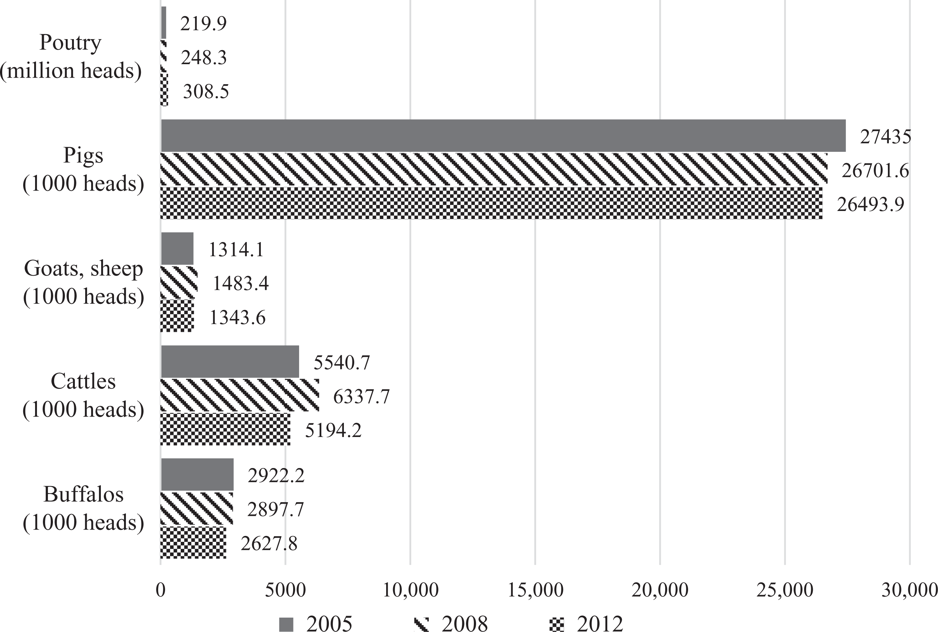
Livestock populations for 2005–2012. Source: GSO (2012a).

Unfortunately, few relevant studies have been carried out to measure the technical efficiency (TE) of livestock production activities in general and among specific product areas. Among the studies undertaken, however, some important findings have been made. Within the research remit of the International Livestock Research Institute, Akter et al. (2003) used stochastic frontier analysis (SFA) to estimate the TE of poultry and pig production in Vietnam during 1999. The results reveal estimated TE of 76.8% in the north of the country and 69.4% in the south for poultry production, and 73% in the north and 77.9% in the south for pig production. In its project report, Agrifood Consulting International (2001: 4-1) stated that “There appear to be diseconomies of scale in livestock production, with profits increasing at a slower rate as inventories and revenues increase. This implies that the efficiency levels on smaller farms, based on raising local animals with low cost feedstuffs are higher than those on larger farms employing intensive high quality feed production techniques.”

Within its “Master plan for developing the agricultural sector until 2020 with a vision for 2030,” the Ministry of Agriculture and Rural Development (MARD, 2012) states it will encourage the development of large livestock farms of an appropriate production scale. In general, both the modernization and industrialization of production are consistent demands within transition economies; however, progress on this often depends on the specific characteristics of each sector involved, as well as the production practices themselves. This study, therefore, has three objectives and uses three related methodologies: (i) To measure the TE of livestock production in Vietnam on a regional basis, by applying the bootstrapping data envelopment analysis (DEA) method. TE will then be adjusted in accordance with the meta-frontier, to identify regional differences. (ii) To estimate technical inefficiency factors using repeatedly bootstrapped truncated regressions. And (iii) to measure changes in productivity performance levels and the composition of these changes using the bootstrapping Malmquist index (Figure 1).

Methodology

TE and inefficiency factors using two-stage DEA

Farrell (1957) illustrated the concepts of efficiencies using the example of a firm whose work process has two inputs (x ₁ and x ₂) and one output (q), and using the assumption of constant returns to scale (CRS). As illustrated in Figure 2, TE is measured on an input-orientation basis, which reflects the ability of a firm to reduce inputs without changing the outputs. TE is determined by comparing the actual production set (point P) and the fully efficient production set (point Q), Q being a point on the isoquant SS′. Then, TE is measured using the ratio: TE = 0Q/0P, with the resulting TE values falling between 0 and 1. The distance QP represents technical inefficiencies, and inputs can be reduced without any change in the outputs. An alternative approach, known as the output-oriented measure, measures the ability of a firm to increase outputs without changing inputs. However, only the input-oriented measure is described and used in this study.

Figure 2.

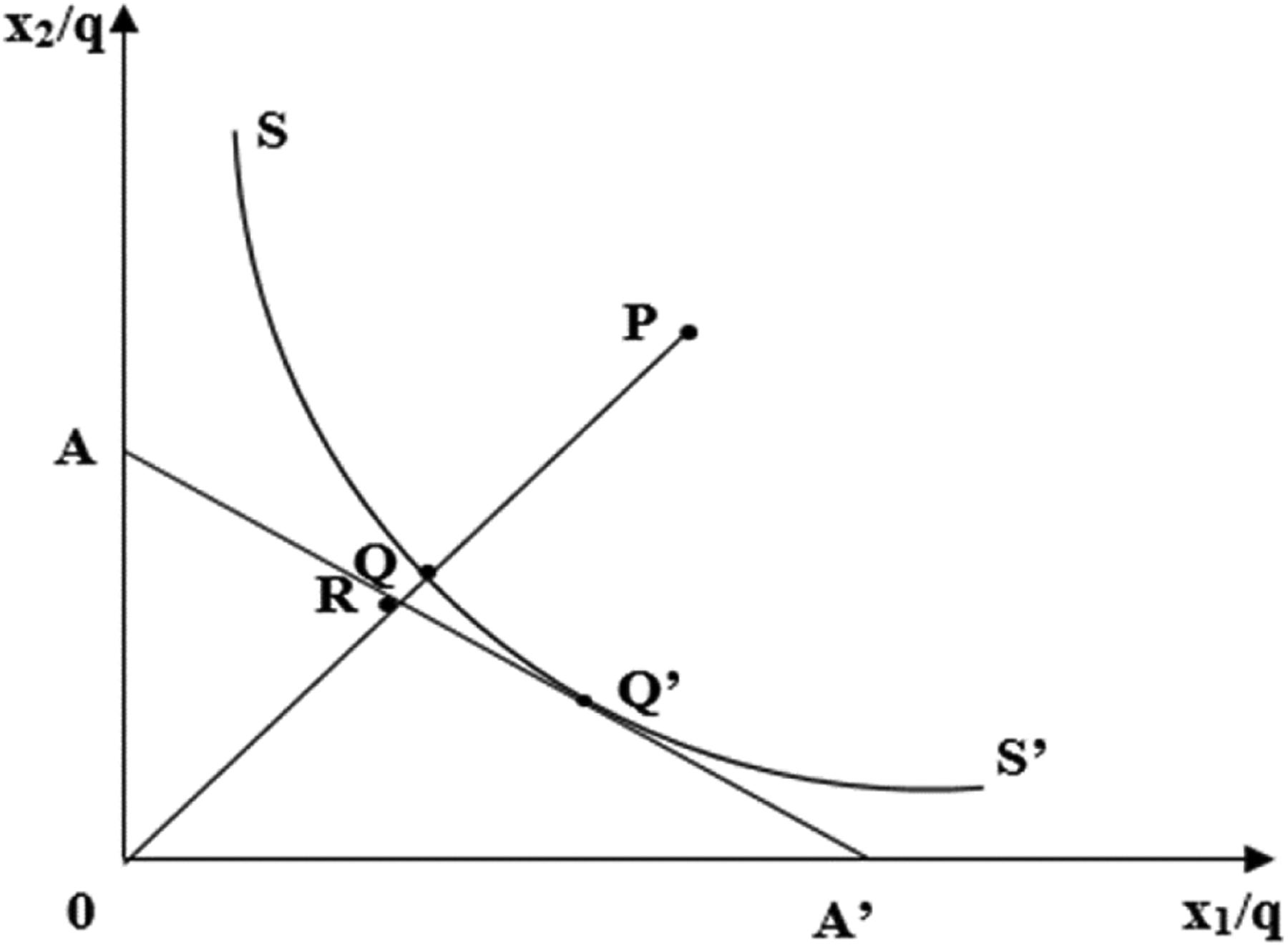
Technical and allocative efficiencies. Source: Coelli et al. (1998).

To measure TE, Two popular approaches such as SFA and DEA are used to measure TE. While the first method is based on an estimation of TE using parametric techniques, the second uses mathematical, nonparametric techniques to measure efficiency. To estimate functional relationships between outputs and inputs, SFA requires assumptions to exist on specific production function forms and the distribution of the inefficiency term (Coelli, 1995). Different geographical regions may be characterized by varying production technologies; and therefore, SFA may require many assumptions to be made for different regions. On the other hand, one of the advantages of DEA is that it is based on a nonparametric technique, and so no assumptions are required regarding production function form, allowing one to use the same methodology to measure TE across different regions. Due to its focus on regional differences, this study will apply the DEA method to measure and compare TE and also productivity performance and composition changes across Vietnamese regions.

Let us assume the production set includes K inputs and M outputs in each of I decision units (say a firm). Then, x_i is the K × 1 vector of inputs of the ith firm, q_i is the M × 1 vector of outputs of the ith firm, X is a K × I input matrix and Q is an M × I output matrix. The envelopment forms for the input-oriented DEA method, and using CRS and variable returns to scale (VRS) assumptions, are shown in Table 1. To compare the actual production scale with the optimal scale, the concept of scale efficiency (SE) is introduced. SE is given by the ratio between TE under CRS (TE_CRS), and TE under TE_VRS, as follows:

Table 1.

Input-oriented DEA using CRS and VRS assumptions^a.

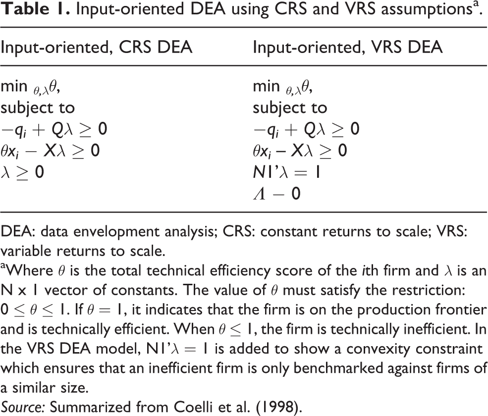
Input-oriented, CRS DEA	Input-oriented, VRS DEA
min _θ,λθ, subject to −q_i + Qλ ≥ 0 θx_i − Xλ ≥ 0 λ ≥ 0	min _θ,λθ, subject to −q_i + Qλ ≥ 0 θx_i – Xλ ≥ 0 N1’λ = 1 Λ − 0

DEA: data envelopment analysis; CRS: constant returns to scale; VRS: variable returns to scale. ^aWhere θ is the total technical efficiency score of the ith firm and λ is an N x 1 vector of constants. The value of θ must satisfy the restriction: 0 ≤ θ ≤ 1. If θ = 1, it indicates that the firm is on the production frontier and is technically efficient. When θ ≤ 1, the firm is technically inefficient. In the VRS DEA model, N1’λ = 1 is added to show a convexity constraint which ensures that an inefficient firm is only benchmarked against firms of a similar size.

Source: Summarized from Coelli et al. (1998).

S E = T E_{C R S} / T E_{V R S} .

After measuring TE, it is useful to identify technical inefficiency factors in a two-stage DEA, in order to define how TE is impacted in practice. Based on previous works in this area (Simar and Wilson, 2000, 2007), Simar and Wilson (2011) stated that only two statistical models, truncated regression and ordinary least squares (OLS) regression, are well enough defined and of use for a two-stage DEA. However, OLS estimation is consistent only under very peculiar and unusual assumptions. As a result, truncated regression with bootstrapping is the most appropriate method to use for this study. During the second stage of the analysis, the bootstrap values for TE resulting from the first stage were bootstrapped again using the truncated regressions, to explore the impacts of technical inefficiency factors.

Meta-frontier and regional differences

After measuring TE, one may want to compare this value across regions. However, due to differences in production environment characteristics, regions may have different production technology sets; therefore, a comparison of regions will only be meaningful if production frontiers are similar. Based on the meta-production function concept defined in previous studies (Hayami and Ruttan, 1970; Prasada Rao et al., 2003), O’Donnell et al. (2008) introduced the concept of meta-frontier or meta-technology to take into account all regional frontiers. To illustrate, let us say the meta-frontier M in Figure 3 is determined by three regional frontiers: k1, k2, and k3. Point A is an observation of region k3, so:

The TE of A in region k3 can be calculated by: $T E_{A}^{k 3} = \frac{P B}{P A};$

The TE of A in all regions (meta) can be calculated by: $T E_{A}^{*} = \frac{P C}{P A};$ and

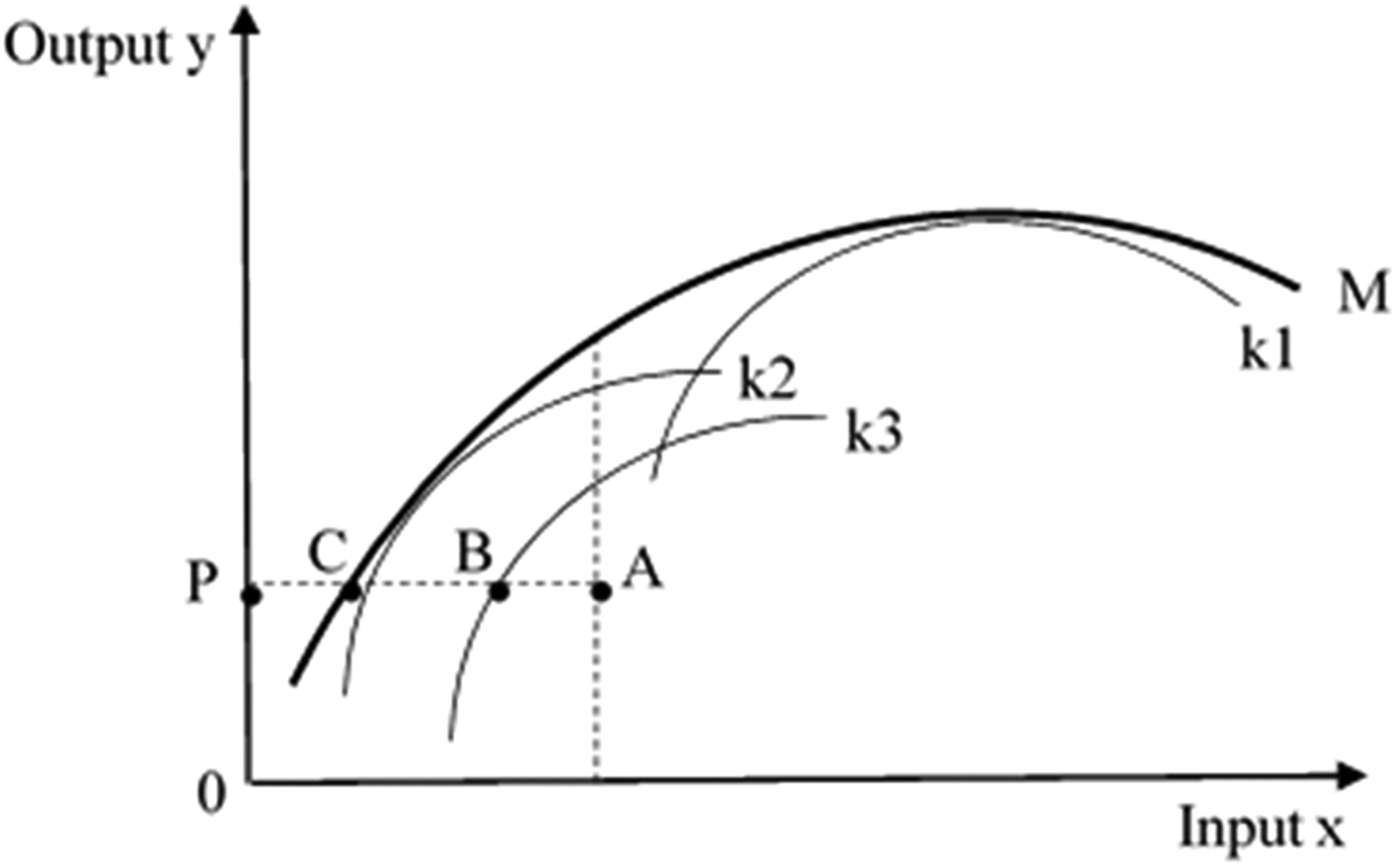
The meta-technology ratio (MTR) of A can be calculated using: $M T R_{A} = \frac{T E_{A}^{*}}{T E_{A}^{k 3}} = \frac{P C / P A}{P B / P A} = \frac{P C}{P B} .$

Figure 3.

Regional frontiers and the meta-frontier. Source: Adapted from O’Donnell et al. (2008).

Basically, differences in TE between groups (regions) can be measured using the following steps: (i) by measuring TE with respect to the group (region) frontiers K, using DEA to analyze the data sets (x, y) obtained by observations within the region, say TE^K(x, y), (ii) by measuring TE with respect to the meta-frontier by using DEA to analyze the data set (x, y) obtained and by pooling all the observations from all the regions, TE*(x, y), and (iii) by calculating the MTRs between group frontiers and the meta-frontier:

M T R^{k} (x, y) = \frac{T E^{*} (x, y)}{T E^{k} (x, y)} .

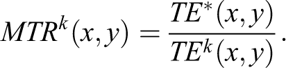
The MTR is always equal to or greater than 0 and less than or equal to 1. If the MTR is equal to 1, it means the regional technology frontier coincides with the meta-technology frontier for the input and output vectors x and y (Prasada Rao et al., 2003).

Productivity measurement using the Malmquist index

The Malmquist index measures total factor productivity (TFP) growth, with TFP defined using a distance function, where an output distance function is used to consider a maximum proportional expansion of the output y, given the input x. The TFP change (tfpch) over time: t + 1 and t can be decomposed into (1) TE change or catching-up effect and (2) technical change or shifts in the frontier or in innovation levels, as follows:

m = {[\frac{d^{t} (x^{t + 1}, y^{t + 1})}{d^{t} (x^{t}, y^{t})} x \frac{d^{t + 1} (x^{t + 1}, y^{t + 1})}{d^{t + 1} (x^{t}, y^{t})}]}^{1 / 2} = \frac{d^{t + 1} (x^{t + 1}, y^{t + 1})}{d^{t} (x^{t}, y^{t})} x {[\frac{d^{t} (x^{t + 1}, y^{t + 1})}{d^{t + 1} (x^{t + 1}, y^{t + 1})} x \frac{d^{t} (x^{t}, y^{t})}{d^{t + 1} (x^{t}, y^{t})}]}^{1 / 2},

e f f c h (TE change) = \frac{d^{t} (x^{t + 1}, y^{t + 1})}{d^{t} (x^{t}, y^{t})},

t e c h c h (technical change) = {[\frac{d^{t} (x^{t + 1}, y^{t + 1})}{d^{t + 1} (x^{t + 1}, y^{t + 1})} x \frac{d^{t} (x^{t}, y^{t})}{d^{t + 1} (x^{t}, y^{t})}]}^{1 / 2},

t f p c h = e f f c h \times t e c h c h .

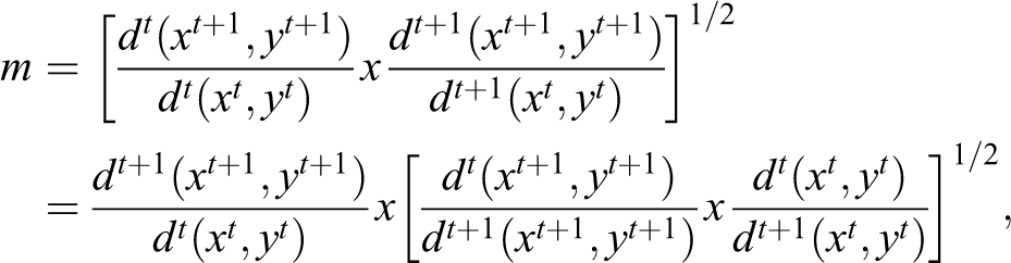
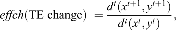
A value of m greater than one indicates a growth in productivity. A value of m > 1 reflects productivity improvement, m < 1 indicates a decline in productivity, and m = 1 reflects no improvement. TE change (effch) can be further decomposed into pure efficiency change (pech) and scale change (sech): effch = pech × sech. The pech component reflects the real or genuine efficiency change associated with the adoption of technology, while sech represents changes that occur due to changes in size or scale of the decision making units.

Bootstrap formulation

To avoid bias in the results when estimating TE scores using DEA, Simar and Wilson (1998), based on the work of Efron (1979), proposed a bootstrap strategy for analyzing the sensitivity of efficiency measures to sampling variations, providing confidence intervals and corrections for the bias inherent in the DEA procedure. The principal bootstrap technique follows the following basic steps: (i) construct an empirical probability distribution of the sample, (ii) resample the data set a specified number of times, (iii) calculate the specific statistic from each sample, and (iv) find the standard deviation of the distribution of that statistic. The bootstrap technique was employed in this study for all the computations, including measuring TE, identifying inefficiency factors in truncated regressions, and measuring the Malmquist index.

Data analysis

Since 2002, the Vietnam Access to Resources Household Survey (VARHS) has been carried out every 2 years across the country. The households surveyed are updated and replaced after each survey which provides a panel data set covering different periods. However, because of household changes, creating panel data for livestock production over a number of years is quite difficult. As a result, this study analyzes a 4-year period using the VARHS data set for 2008 to 2012 (GSO, 2008, 2010, 2012b). Regions in Vietnam can be divided into eight, geographically; however, VARHS was conducted across 12 provinces, representing only seven regions. Due to this limitation, in this study, only seven of eight regions are analyzed. After excluding households without livestock or which did not satisfy all the common features, the total number of households remaining was 2477. The regional breakdown was Red River Delta (255), Northeast (579), Northwest (605), North Central Coast (183), South Central Coast (214), Central Highlands (503), and Mekong River Delta (138). To avoid results bias due to differences in sample sizes (Alirezaee et al., 1998; Andor and Hesse, 2011; Staat, 2001; Zhang and Bartels, 1998) across regions, an ap function (Wilson, 2008) was employed to detect and drop three outliers from the Mekong River Delta, leaving this region with 135 observations. The number of observations in each of the other regions was randomly chosen as being 140. The number of observations used to measure TE in each region was between 135 and 945.

One critical aspect of this study is the approach taken to measure livestock output levels. The difficulty lies in trying to describe livestock numbers of varying species as a single figure, one that expresses the total number present. Based on the work of the FAO (1979), Jahnke (1982) suggested using the tropical livestock unit (TLU). TLU conversion factors are based on weight and feed supply for each species and constitute a compromise between different common practices. Specifically, this study followed Jahnke (1982) using weighting to calculate total livestock output levels as follows:

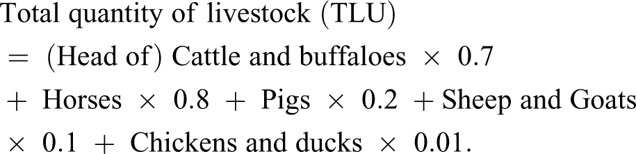
\begin{array}{l} Total quantity of livestock (TLU) = (Head of) Cattle and buffaloes \times 0. 7 + Horses \times 0. 8 + Pigs \times 0. 2 + Sheep and Goats \times 0. 1 + Chickens and ducks \times 0.0 1 . \end{array}

The TLU was used as the only output into the DEA. The six model inputs included (i) family labor (hours), (ii) feed (home produced), (iii) feed (bought), (iv) breeding stock (insemination), (v) veterinary services and medicine, and (vi) others (all in 1000 VND). From the VARHS results, the area of livestock production covered was not clear and missing many observations. The possible reason was that households in the study area kept their livestock in a number of different locations, including alongside annual crops, in long-term tree plantations, grass fields, alongside gardens and/or ponds, or even on residential land. Even in the results from the second stage DEA, the pooled area does not impact upon TE; this is the reason why area was not used as an input in the production set.

In the second stage, the TE bootstrap scores were used as the dependent variable, with 11 other variables used as independent variables including (i) gender of household head (1 = male, 0 = female), (ii) age of household head (year), (iii) married status of household head (1 = single, 2 = married, 3 = widowed, 4 = divorced, 5 = separated), (iv) education level of household head (0 = never went to school or did not finish first grade, 1–12: grades), (v) household size (number of members), (vi) natural and biological shocks (0 = no, 1 = yes), (vii) economic shocks (0 = no, 1 = yes), (viii) shocks to household members (0 = no, 1 = yes), (ix) share of livestock income as a proportion of total agricultural income (%), (x) share of nonfarm income as a proportion of total income (%), (xi) production scale (1 = if TLU < 0.5, 2 = if 0.5 ≤ TLU < 1, 3 = if 1 ≤ TLU < 2, 4 = if 2 ≤ TLU < 3, 5 = if 3 ≤ TLU < 4, 6 = if 4 ≤ TLU < 5, 7 = if 5 ≤ TLU < 6, 8 = if 6 ≤ TLU < 7, 9 = if 7 ≤ TLU < 10, and 10 = if 10 ≤ TLU). To measure changes in productivity, TE, and technology, the one output and six inputs stated above were included in the panel data for 2008–2012.

The study employed the boot.sw98 function to measure bootstrapping TE while malmquist.components and malmquist functions were used to measure changes in productivity and the composition of these changes. All these functions belong to the Frontier Efficiency Analysis with R (FEAR) package developed by Wilson (2008). To identify the technical inefficiency factor, truncated regressions are estimated in Stata. All the processes used to measure TE, truncated regressions, and Malmquist indexes were bootstrapped over 2000 replications, with an α value of 0.05 used to estimate the statistical sizes of the confidence intervals.

Results and discussion

Regional differences in TE

As summarized in Table 2, under both the CRS and VRS assumptions, TE scores for livestock production across all regions are quite low. Within each region, the bootstrapping values for VRS TE vary from around 17% to 40%. This means that inputs are able to reduce from 83% to 60% without changing outputs. On the other hand, SE levels are very low; for instance, the SE value for the Central Highlands is only 6%, when compared to its optimal scale. However, as mentioned previously, production technology differences may exist across regions, meaning it is not appropriate to compare TEs. As a result, it is necessary to adjust TEs to meta-frontier values which include all regional frontiers, as illustrated in Figure 4. Using meta-frontier frontier¹, all the observations used to measure regional TE are measured again as pooled data. After that, the MTR can be calculated and be used to compare regions. Table 3 provides a detailed description of these results.

Table 2.

Technical efficiency (Eff), bias-corrected TE (Eff.bc) scores when using VRS, CRS assumptions, and SE.

Region	VRS		CRS		SE
Region	Eff	Eff.bc	Eff	Eff.bc	Eff	Eff.bc
Red River Delta	0.5243	0.3607	0.2109	0.1102	0.4023	0.3055
Northeast	0.2734	0.1723	0.1197	0.0623	0.4378	0.3616
Northwest	0.3460	0.2405	0.1083	0.0584	0.3130	0.2428
North Central Coast	0.4795	0.3536	0.1334	0.0679	0.2782	0.1920
South Central Coast	0.5668	0.4026	0.2715	0.1368	0.4790	0.3398
Central Highlands	0.3544	0.2481	0.0379	0.0159	0.1069	0.0641
Mekong River Delta	0.3950	0.2514	0.1568	0.0811	0.3970	0.3226

CRS: constant returns to scale; SE: scale efficiency; VRS: variable returns to scale.

Figure 4.

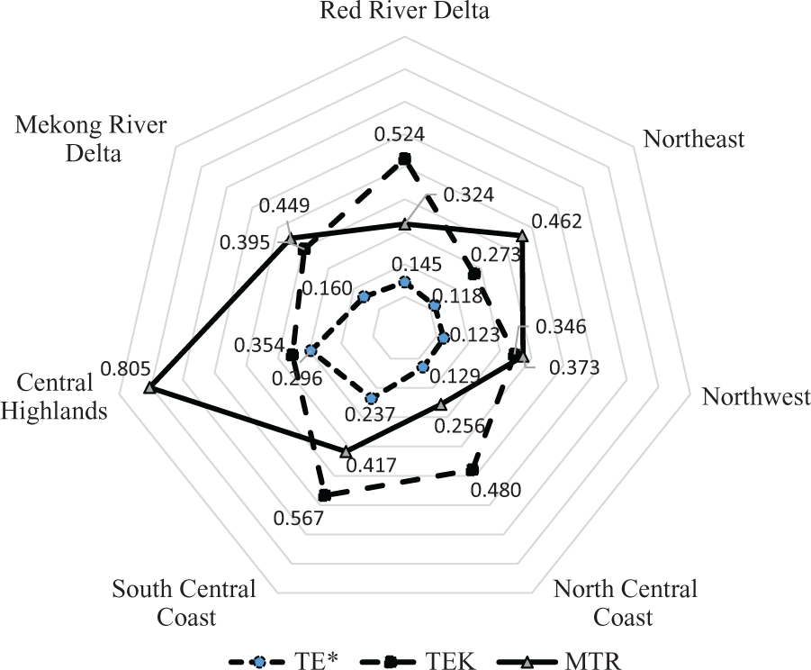
Regional differences in technical efficiency between regional frontier (TE^K), meta-frontier (TE*), and meta-technology ratio using variable returns to scale.

Table 3.

Description of differences in TE between regional frontiers (TE^K), meta-frontier (TE*), and the MTR using VRS.

Region	Variable	Obs	Mean	Std. dev	Min	Max
Red River Delta	TE*	135	0.1452	0.1786	0.0111	1
	TE^K	135	0.5243	0.3843	0.0208	1
	MTR	135	0.3237	0.2094	0.0423	1
Northeast	TE*	135	0.1176	0.1810	0.0130	1
	TE^K	135	0.2734	0.3053	0.0333	1
	MTR	135	0.4616	0.1877	0.0478	1
Northwest	TE*	135	0.1228	0.1374	0.0186	1
	TE^K	135	0.3460	0.2594	0.0904	1
	MTR	135	0.3729	0.1890	0.0429	1
North Central Coast	TE*	135	0.1294	0.1428	0.0232	1
	TE^K	135	0.4795	0.3060	0.0865	1
	MTR	135	0.2562	0.1161	0.1276	1
South Central Coast	TE*	135	0.2366	0.2363	0.0377	1
	TE^K	135	0.5668	0.3459	0.0900	1
	MTR	135	0.4172	0.2275	0.0554	1
Central Highlands	TE*	135	0.2959	0.2898	0.0203	1
	TE^K	135	0.3544	0.3063	0.0251	1
	MTR	135	0.8049	0.1562	0.3731	1
Mekong River Delta	TE*	135	0.1604	0.2288	0.0049	1
	TE^K	135	0.3950	0.3789	0.0111	1
	MTR	135	0.4489	0.2537	0.0064	1

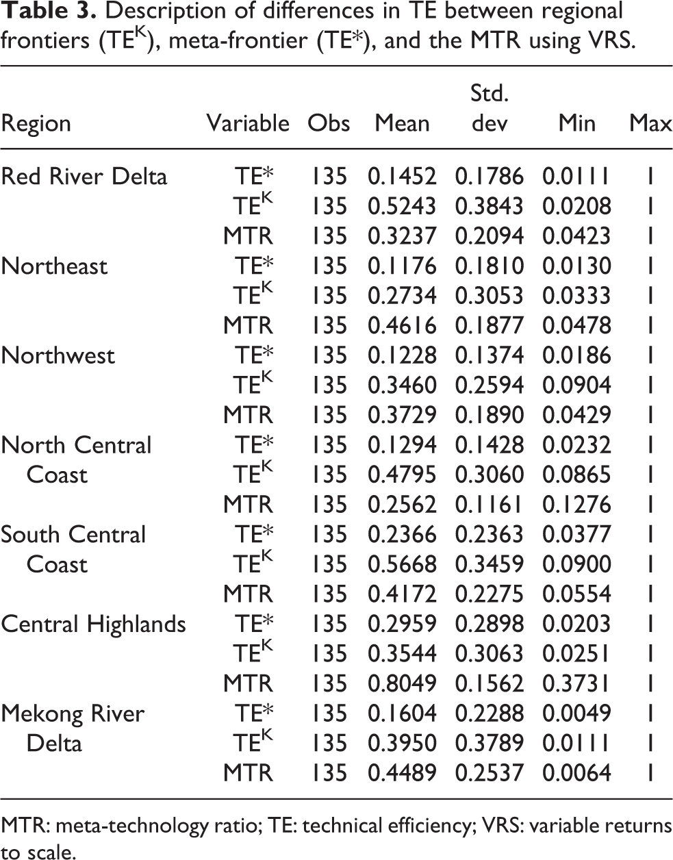
MTR: meta-technology ratio; TE: technical efficiency; VRS: variable returns to scale.

The MTR values show that the Central Highlands region is the most efficient, at 80.5%, when compared to other regions in the country, while the North Central Coast is the least efficient region for livestock production, at only 25.6%. Unfortunately, no other studies have been carried out with which to compare these results, due to differences in the approaches used to measure livestock product outputs. Furthermore, it would be inappropriate to use the TE of a specific year to represent the whole picture in terms of livestock production over a number of years, due to the risk of livestock types varying, which may lead to an immediate decline in TE, as described below.

Technical inefficiency factors

Table 4 summarizes the results of the truncated regression analysis carried out between the bootstrapped TE values and the other explanatory variables. From the data, production scale—based on the scale of outputs—has a significant impact on TE levels. Being significant at 1%, larger production scales lead to lower TE values across all regions. This is an interesting result and aligns with the conclusions of Agrifood Consulting International (2001): Households with smaller-scale livestock production activities and using lower-cost home-sourced feedstuffs are more efficient than those with larger-scale production activities and buying-in high-quality feed. Another reason for this is that livestock production activities on larger-scale farms may be more vulnerable because livestock diseases can spread on a large scale.

Table 4.

Statistical summary of the truncated regression model results across the study regions.

Dependent variable: Bias_corrected_TE_VRS ^a	Red River Delta	Northeast	Northwest	North Central Coast	South Central Coast	Central Highlands	Mekong River Delta	Whole country
Number of observations	135	135	135	135	135	135	135	945
Wald χ²	132.06	128.57	73.43	81.61	40.23	60.03	37.51	207.89
Prob > χ²	0.0000	0.0000	0.0000	0.0000	0.0000	0.0000	0.0000	0.0000
Log likelihood	31.0040	94.4914	86.8461	52.1562	25.1478	50.2960	23.9748	656.4135
	Coefficients
Gender of household head	0.1033	0.0166	−0.0821^b	0.0521	0.0252	−0.0045	−0.0503	0.0014
Age of household head	−0.0022	−0.0005	−0.0021^c	−0.0005	0.0020	−0.0001	−0.0006	0.0002
Married status of household head	0.0115	0.1253^c	0.1530^d	0.0001	−0.0893^b	0.0220	−0.0299	0.0167
Education of household head	0.0046	0.0052^b	−0.0038	0.0090	−0.0068	−0.0022	−0.0039	−0.0015
Household size	−0.0006	−0.0174^d	−0.0059	−0.0042	−0.0059	−0.0020	0.0151	−0.0006
Natural and biological shocks	−0.0682	−0.0195	−0.0330	0.0396	0.0017	−0.1061^d	−0.0573	−0.0307^d
Economic shocks	−0.1678^d	−0.0143	−0.0771^c	0.1394^c	0.0270	0.0474	−0.1258	0.0003
Shocks to household members	0.0631	−0.0728^c	0.1547	−0.0483	0.0340	−0.0086	0.1585	−0.0003
Share of livestock income in agriculture income	−0.1526^c	−0.1795^d	−0.1042	−0.1211^b	−0.1529^c	−0.3501^d	−0.1048^c	−0.1256^d
Share of nonfarm income in total income	0.0728	0.1314^d	0.1356^d	0.2444^d	0.2474^d	0.2202^d	0.0888	0.0410^d
Production scale	−0.0671^d	−0.0411^d	−0.0368^d	−0.0591^d	−0.0484^d	−0.0485^d	−0.0345^d	−0.0231^d
_cons	0.4854	0.1024	0.3154^c	0.2664^b	0.5379^d	0.3717^d	0.4906^d	0.1815^d

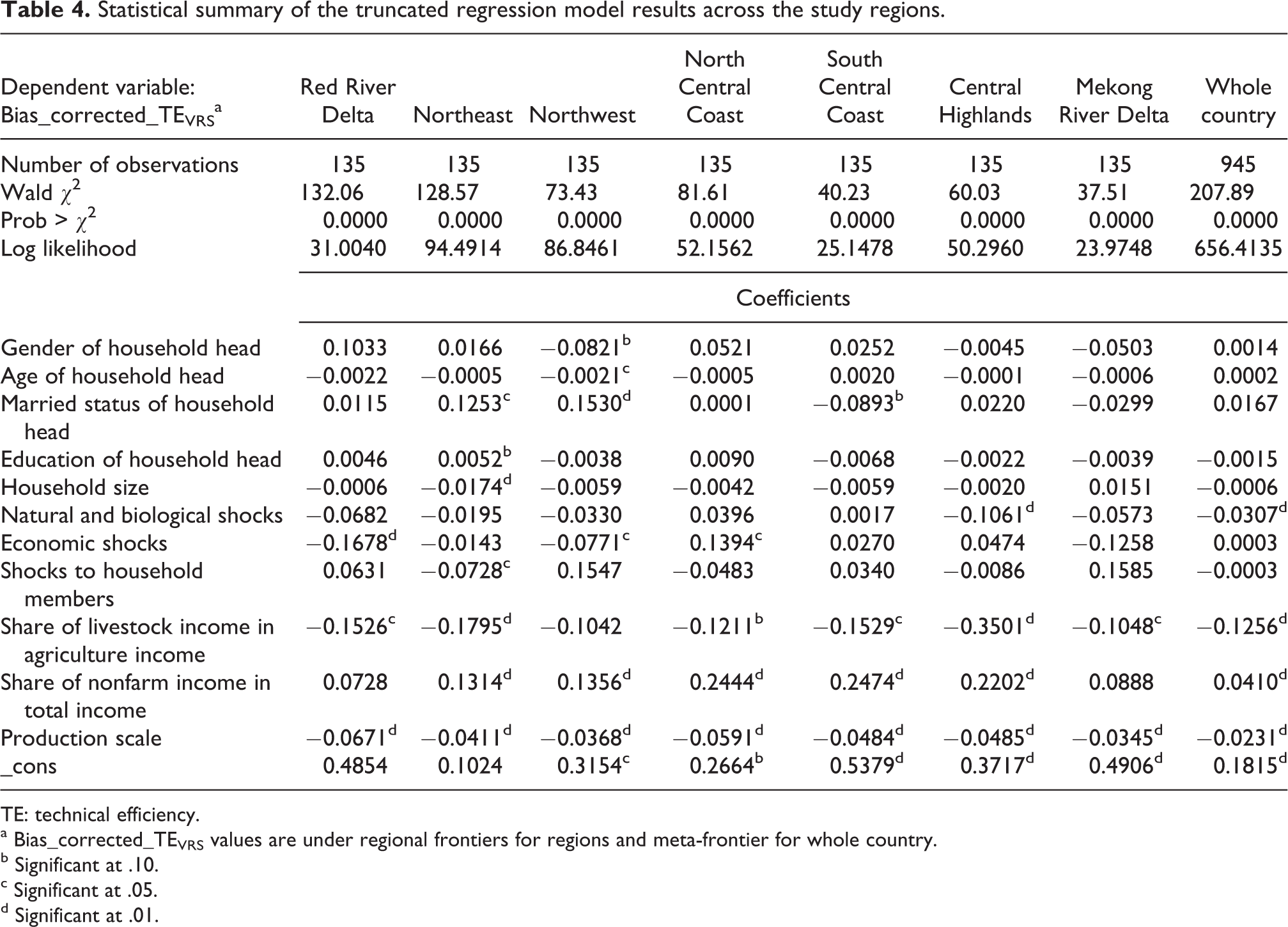
TE: technical efficiency.

^a Bias_corrected_TE_VRS values are under regional frontiers for regions and meta-frontier for whole country.

^b Significant at .10.

^c Significant at .05.

^d Significant at .01.

Although natural and biological shocks, including livestock diseases such as cattle plague or poultry flu, do not have a significant impact across all regions, they do have a significant impact on TE levels in the Central Highlands region. Meanwhile, economic shocks such as changes in input and output prices, unemployment and others, have varying impacts across regions. In two of the three regions impacted, this factor is negatively related to TE, while in another region, they have a positive impact on TE. Other notable impacts on TE levels are the share of livestock income in total agricultural income and the share of nonfarm incomes as a proportion of total household incomes. Households that depend heavily on livestock rearing for their agricultural income have lower TE values for their livestock production activities. Meanwhile, households with higher share of nonfarm incomes are also more efficient than the other households in terms of their livestock production activities.

Changes in productivity, TE, and technology

Livestock production activities, in practice, face too many types of risks; therefore, their TEs also vary across regions and other years. Table 5 examines the changes in productivity levels (tfpch) and the composition of the changes between 2008 and 2012. Positive estimates for efficiency change (effch) are interpreted as representing technical diffusion, while positive estimates for technology change (techch) are seen as representing an expansion of technology frontiers. Over the 4-year period, livestock productivity levels across all regions show a decline, in spite of the offsetting impacts of efficiency and technology changes. In the case of the Central Highlands, however, efficiency levels recover very quickly, that is, livestock diseases may have resulted in low efficiency levels in 2008, after which TE levels increase rapidly once the diseases are under control. However, the high and positive change in efficiency levels is not sufficient to compensate for productivity losses when technological change is also low.

Table 5.

Summary of changes in productivity, technical efficiency, and technology^a.

Region	tfpch	Effch	Techch	pech	sech
Red River Delta	0.996	0.726	1.371	1.313	0.553
Northeast	0.623	1.711	0.364	0.986	1.735
Northwest	0.508	1.283	0.396	1.056	1.215
North Central Coast	0.406	0.253	1.606	1.273	0.199
South Central Coast	0.820	1.315	0.623	1.943	0.677
Central Highlands	0.260	20.231	0.013	2.092	9.670
Mekong River Delta	0.414	0.072	5.711	0.474	0.153
Whole country	0.544	3.670	0.148	1.589	2.310

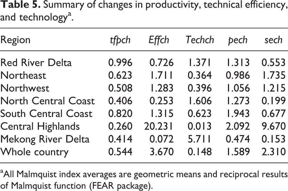
^aAll Malmquist index averages are geometric means and reciprocal results of Malmquist function (FEAR package).

The Mekong River Delta is another contrasting case. Here, productivity levels fall due to negative changes in efficiency levels; however, thereafter, the rate of expansion in technology frontiers—through the application of new livestock production technologies—is quite high, offsetting the negative impacts of efficiency change. Taking a closer look, efficiency changes can be decomposed into two subcomponents: pure efficiency change (pech) and SE change (sech). Other things being similar, changes in both pure efficiency and SE offset each other in terms of their contribution to efficiency changes, except in the Central Highlands and Northwest. For example, in the Central Highlands, SE changes have a more important impact on efficiency levels than changes in pure efficiency.

Conclusions

Generally, most of the results produced from this examination of TE and productivity performance levels paint a generally negative picture of livestock production activities across Vietnamese regions. Efficiency improvements in five of the eight regions may be a result of a reduction in the negative impacts of natural and biological shocks over the period 2008–2010, when compared to the period 2006–2008, as described by GSO (2010). However, these improvements do not account for the poor livestock production performance shown generally. While households with small-scale production activities have advantages in terms of using lower-cost feedstuffs and having higher efficiency levels, households more dependent on the livestock sector for their incomes are more vulnerable and face greater risks. These results would seem to challenge the government’s efforts to expand production scales by increasing the size of livestock farms. However, one of the limitations of this study is that it only measures TE levels and other relevant indices based on a household survey, meaning other livestock production forms, such as commercial farms or state farms, are not included. Therefore, it may be inappropriate to draw conclusions as to which types of farm are more efficient among larger-scale livestock farms. Furthermore, the specific approach used here to measure livestock outputs is based on FAO (1979) and Jahnke (1982), and this may make it difficult to compare these results with other studies that used different approaches. Finally, livestock production activities face many different types of risk, so it may be inappropriate to use the results from specific years or specific regions to represent the whole sector over a number of years and across all of Vietnam’s regions.

Footnotes

Declaration of conflicting interests

The author(s) declared no potential conflicts of interest with respect to the research, authorship, and/or publication of this article.

Funding

The author(s) received no financial support for the research, authorship, and/or publication of this article.

Note

References

Agrifood Consulting International (2001) Policy Option for Using Livestock to Promote Rural Income Diversification and Growth in Vietnam. Hanoi: International Food Policy Research Institute.

Akter

Jabbar

Ehui

(2003) Competitiveness and efficiency in poultry and pig production in Vietnam (Socio-economics and Policy Research Working Paper 57). Kenya: International Livestock Research Institute.

Alirezaee

Howland

Van De Panne

(1998) Sampling size and efficiency bias in data envelopment analysis. Journal of Applied Mathematics & Decision Sciences 2(1):51–64.

Andor

Hesse

(2011) A Monte Carlo simulation comparing DEA, SFA and two simple approaches to combine efficiency estimates. CAWM Discussion Paper, University of Münster, 51. Available at: http://econstor.eu/bitstream/10419/51383/1/672474034.pdf

Anh

(2012) Vietnam Feed Industry. Hanoi: Swiss Business Hub ASEAN/Vietnam Office.

Coelli

(1995) Recent developments in frontier modeling and efficiency measurement. Australian Journal of Agricultural Economics Research 39:219–245.

Coelli

Prasada Rao

Battese

(1998) An Introduction to Efficiency and Productivity Analysis. Boston: Kluwer Academic Publishers.

Efron

(1979) Bootstrap methods: another look at the Jackknife. The Annals of Statistics 7:1–26.

Farrell

(1957) The measurement of productive efficiency. Journal of the Royal Statistical Society, Series A (General) 120(3):253–290.

10.

Food and Agriculture Organization of the United Nations (FAO) (1979) Production Yearbook. Rome: FAO.

11.

Food and Agriculture Organization of the United Nations (FAO) (2005) Livestock sector brief - Vietnam. Rome: FAO.

12.

General Statistics Office of Vietnam (GSO) (2008) Vietnam Access to Resources Household Survey. Hanoi: Statistical Publishing House.

13.

General Statistics Office of Vietnam (GSO) (2010) Characteristics of the Vietnamese Rural Economy: Evidence from a 2010 Rural Household Survey in 12 Provinces of Vietnam. Hanoi: GSO.

14.

General Statistics Office of Vietnam (GSO) (2012a) Statistical Database. Hanoi: GSO.

15.

General Statistics Office of Vietnam (GSO) (2012b) Vietnam Access to Resources Household Survey. Hanoi: Statistical Publishing House.

16.

Hayami

Ruttan

(1970) Agricultural productivity differences among countries. The American Economic Review 60(5):895–911.

17.

Jahnke

(1982) Livestock Production Systems and Livestock Development in Tropical Africa. Kiel: Kieler Wissenschaftsverlag Vauk.

18.

Minister of Agriculture and Rural Development (MARD) (2012) The 2011 – 2020 Restructuring Scheme on Agriculture Sector. Hanoi: MARD.

19.

O’Donnell

Prasada Rao

Battese

(2008) Metafrontier frameworks for the study of firm-level efficiencies and technology ratios. Empirical Economics 34:231–255.

20.

Prasada Rao

O’Donnell

Battese

(2003) Metafrontier functions for the study of inter-regional productivity differences. CEPA Working Papers Series (WP012003), School of Economics, University of Queensland, Australia.

21.

Simar

Wilson

(1998) Sensitivity analysis of efficiency scores: how to bootstrap in nonparametric frontier models. Management Science 44(11):49–61.

22.

Simar

Wilson

(2000) Statistical inference in nonparametric frontier models: the state of the art. Journal of Productivity Analysis 13(1):49–78.

23.

Simar

Wilson

(2007) Estimation and inference in two-sage semi-parametric models of production processes. Journal of Econometrics 136:31–64.

24.

Simar

Wilson

(2011) Two-stage DEA: Caveat emptor. Journal of Productivity Analysis 36:205–218.

25.

Staat

(2001) The effect of sample size on the mean efficiency in DEA: comment. Journal of Productivity Analysis 15:129–137.

26.

Wilson

(2008) FEAR: a software package for frontier efficiency analysis with R. Socio-Economic Planning Sciences 42(4):247–254.

27.

Zhang

Bartels

(1998) The effect of sample size on mean efficiency in DEA with an application to electricity distribution in Australia, Sweden and New Zealand. Journal of Productivity Analysis 9:187–204.