A computational study of the aerodynamic influence on the heavy vehicle Araba body model

Abstract

This paper presents a novel design and computational analysis for a heavy vehicle model, named the Araba body, created from the existing Ahmed body. The design was created with various parametric variations, such as the frontal height (h), rounding radius (R), diffuser height (h_d), and slant angle (α). The experimental studies were validated using an existing Ahmed body. Owing to the necessary changes in these parameters, lower drag values were obtained. A Large Eddy Simulation (LES) model was used for the simulations. The vortices were obtained from all cases and analyzed along with the coefficient of drag (C_d) and pressure coefficient for the drag (C_dp). It can be seen that for ‘R′ of 0.3 m had the lowest coefficient of drag (C_d) of 0.12 and the pressure coefficient for the drag (C_dp) of 0.15. The rounding radius had an impact of 2.5% on both the C_d and C_dp. For the ‘h’ parameter, the lowest values of 0.149 (C_d) and 0.117 (C_dp) were obtained at a height(h) of 0.8 m. Similarly, for the ‘h_d’ and ‘α′ parameters, lower drags are obtained at its maximum range; thus, total of 108 cases are obtained. Finally, a complete coefficient of drag (C_d) and the pressure coefficient of drag (Cd_p) is obtained from all 108 computational variations. The results show great potential for enhancing the aerodynamic performance off the computed Araba body.

Keywords

heavy vehicle model aerodynamics CFD numerical simulation araba body

1. Introduction

In the years of technological evolution in the automobile sector, engineers and researchers are creating various design models to improve the optimization of vehicle efficiency, and more research is being conducted to reduce drag. The implementation of computational fluid dynamics (CFD) in the design of new techniques and prototypes has proven to be the most dependable method, such as the Ahmed body,¹ which is one of the most researched simplified geometries in the field of aerodynamic studies.

Various studies have been conducted to validate the numerical models paving the way for advanced research. For instance, Tunay et al.,^2,3 performed a detailed experimental and computational study on vortex shedding from the lower base edge and upper edge of the rear window and determined the wake force characteristics of the Ahmed body. Barros et al.,^4,5 studied the wake and drag of turbulence past a 3D blunt body. Rao et al.⁶ performed a detailed analysis of the two flow states and observed them in the wake of the Ahmed body, which was investigated numerically using the partially averaged navier–stokes (PANS) turbulence model on unstructured meshes.

The changes in the flow state as the back slant angle is varied are well documented by several experimental and numerical analyses along with the yaw angle. Guilmineau et al.⁷ conducted a research investigation of Reynolds averaged Navier–Stokes (RANS) and hybrid RANS-LES turbulence models for the Ahmed body at 25° and 35° slant angles. The RANS turbulence models used are k − ω SST and a hybrid Large Eddy Simulation (LES). For the Detached Eddy Simulation (DES) and Improved Delay Detached Eddy Simulation (IDDES) a hydrid RANS-LES approaches, these models were based on the k − ω model. For a square back ahmed body an initial study carried out by Grandemange et al.⁸ discovered that the wake has a symmetric behavior depending on the timescale; for the reference height and free stream velocity, the oscillation of the wake is found to be weakly related to the shear layer interactions.

The same author Grandemange et al.⁹ determined that the bistability of the wake is not dependent on the Reynolds number for the values up to 2.5 ⋅ 10⁶. Studies performed by Volpe et al.¹⁰ and Fan et al.¹¹ reported that the wake was stabilizing in one of the two symmetric positions with the flow reaching a steady regime, and that the wake was not dependent on the Reynolds number for the values reaching up to 2.5 ⋅ 10⁶. Initial studies of yaw angles were conducted by Grandemange et al.,¹² and further studies were carried out by Bonnavion and Cadot.¹³ Haffner et al.¹⁴ analyzed the effects of yaw and pitch angles, and concluded that there were changes in both the suppressed bimodal wake behavior. At the same instance, the computational studies performed in (URANS) Unsteady Reynolds - averaged Navier stokes by Khalighi et al.,¹⁵ Detached Eddy Simulations (DES) by Guilmineau et al.,⁷ Improved Delayed Detached Eddy Simulations (IDDES) and LES by^16,17 and Large Eddy Simulations (LES) have been used to analyze the flow on the squareback ahmed body.

Delassaux et al.¹⁸ conducted a comparative research study of SST RANS and three hybrid LES approaches with comparison to their experimental data to understand passive control with rounded edges. Buscariolo et al.¹⁹ conducted a parametric study on the effects of diffusers on the Ahmed body in two slant cases: squared back and 25° angle and the peak drag values were achieved. Aguerre et al.²⁰ performed numerical studies using the hybrid RANS-LES turbulence model to analyze the aerodynamics of the Ahmed body, utilizing an incompressible, Newtonian, and unsteady flow solver to compare the results with the velocity profiles and achieved satisfactory agreements with the global aerodynamics data. The authors Naseeb Ahmed Siddiqui and Chaab²¹ performed studies at low Reynolds number and analyzed the flow transition from the high-drag to low-drag regime and obtained results for various recirculation regions at the front and rear ends. Serre et al.²² performed simulations in the Ahmed body for a Reynolds number of 768000 using LES and DES and described the problems of computational cost, time consumption and ease of implementation, in addition to the quality of results.

A few of the most relevant studies for simplified heavy vehicles or bus models were performed by Krajnovice and Davision²³ using the LES turbulent model and described the vortex structures around the heavy body. This model is closely related to the square back Ahmed body with a addition to the radius of 0.15 m at all edges of the body at speeds of up to 40 km/hr for a city bus. Recent studies on the effects of the diffuser compared the drag coefficient between the square back and Hatchbach Ahmed body with a slant angle of 25° to 40°. The results for the best drag value at 10°. Aultman and Duan²⁴ measured both the slant angle from 10° and diffuser angle up to 33.5°. The poor case is obtained at 30° slant angle and 14.7° diffuser.

For the rounding front, the studies were performed by introducing the basic geometry²⁵ and later performed the DES at a slant angle of 25°²⁶ and discovered that the flow was completely different from that of the Ahmed body initial studies. Garcia et al.²⁷ performed a CFD and CNN study on the Ahmed body for a heavy-vehicle setup for both the velocity and pressure fields.

From the above-mentioned literature survey, no study has revealed a design and CFD analysis of a heavy body that can be taken as a reference design. In this study, a reference heavy vehicle is created and named the Araba body. The geometry is a novel design created for heavy vehicles and is a benchmark for commercial heavy vehicles. A primary study on how the vortices are obtained at in the rear end of the Araba body is explained along with a detailed study performed with variations in different parameters such as the frontal height (h), diffuser height (h_d), rounding radius (R) and slant angle (α) and the results are discussed in detail. The parametric case studies show that the design with the R at 0 m, hd at 0.6 m, α at 10°, and h at 0.6 m has a high coefficient of drag 0.461. In contrast, the case with R at 0.3 m, hd at 0.8 m, α at 30°, and h at 0.8m has the lowest drag value of 0.149, showcasing that the limits of the design for the aerodynamics studies, taking into account the commercial conditions of the heavy vehicle designs for which the design can be manufactured.

2. Large-eddy simulation

In Large Eddy Simulation (LES), the governing equations are obtained by applying a spatial filtering operation to the incompressible Navier–Stokes and continuity equations, with the filter width typically related to the local grid resolution. The fundamental principle of LES is to explicitly resolve the large, energy-containing turbulent structures while modeling the smaller, unresolved scales, which are assumed to play a secondary role in the transport of conserved quantities. Accordingly, the flow variables are decomposed into resolved (filtered) and unresolved (subgrid-scale) components, reflecting the fact that, at practical Reynolds numbers, the computational mesh cannot capture the full range of turbulent scales. The filtering operation, or spatial averaging, is therefore performed at a scale consistent with the mesh spacing. Within this framework, the Boussinesq approximation is commonly employed to model the subgrid-scale stresses, assuming that the deviatoric component of the residual stress tensor is proportional to and aligned with the anisotropic part of the resolved strain-rate tensor. The isotropic part of the residual stresses is incorporated into the modified pressure term and represents the unresolved turbulent kinetic energy K_r. As a result, the filtered continuity and filtered Navier–Stokes equations for incompressible flow were obtained from²⁸,²⁹. Wall-adapting local eddy-viscosity (WALE) model was proposed by Nicoud and Ducros³⁰ and since then it has become a standard part of the CFD software as well as some other in-house CFD codes,³¹ Similarly to the Smagorinsky model, the WALE model is also a linear eddy viscosity turbulence model.³²

3. Geometries

In this study, the Araba body was chosen, and the representation of the geometry is shown in Figure 1. The entire length, width, and height of the heavy vehicle were 12023 mm, 3890 mm, and 2880 mm, respectively. A complete detailing of the design is provided in the appendix A. To validate the simulation, height of the frontal region(h), height of the diffuser (h_d), rounding angle at the front (R), and slant angle at the diffuser (α) were alternated and validated. The ranges mentioned in Table 1 are selected due to the restrictions and limitations in real models, for instance, for (α), the ceiling height of the rear region is considered, for the h_d, the limitations are due to the continuous floor of the cabin, for h the drivers seat position and visibility and for R the structural integrity of the Araba body.

Figure 1.

Araba body geometry with dimensions.

Table 1.

Variations of the parameters.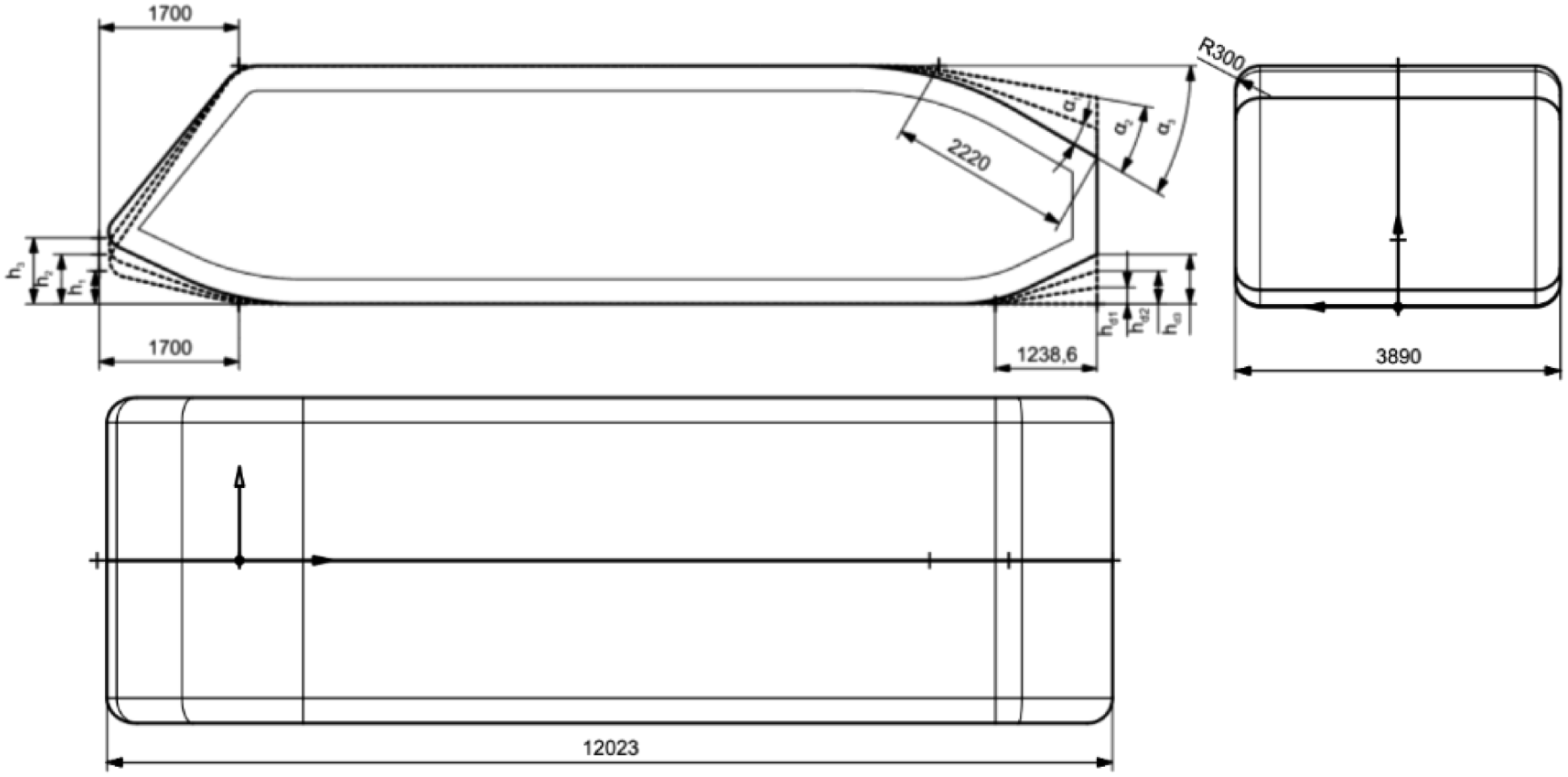

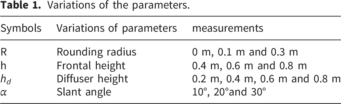
Symbols	Variations of parameters	measurements
R	Rounding radius	0 m, 0.1 m and 0.3 m
h	Frontal height	0.4 m, 0.6 m and 0.8 m
h _d	Diffuser height	0.2 m, 0.4 m, 0.6 m and 0.8 m
α	Slant angle	10°, 20°and 30°

The variations of all the required model are shown in Table 1.

4. Numerical setup

The geometry is placed at a distance of 1.5L from the inlet and intersecting with the symmetric region in the middle. The distance from the rear of the body to the outlet is 7.5L. The subtract operation is used to obtain the heavy vehicle domain flow and since the symmetry set up is used half of the model is simulated, this will reduce the cost of the computations. Air is chosen as the flow medium. LES with WALE model is used in the computation. The time-step for the solver setup is set at a constant value of 0.001 s, with a maximum of 12000 steps used for the simulation. For the inlet, a Reynolds number of 20.4 ⋅ 10⁶ is taken into account for the turbulence study. The boundary conditions are shown in Figure 2, which provides insight into the flow domain. The domain dimensions are X=10L, Y=2L and Z=1L. The frontal area of the Araba body is 5.6 (m²) with a blockage ratio of 2% is obtained showing that the entire block is sufficiently large for the simulation. The velocity inlet was chosen, for the inlet, and the pressure outlet was considered for the outlet. So, the calculated free stream inlet velocity is 26.38 m/s with a kinematic viscosity of air 7.95 ⋅ 10⁻⁵ (m²/s). The Z=0 plane was defined as a symmetry plane with the opposed wall and the ceiling plane also being defined as such, the Ahmed body itself was defined as wall.

Figure 2.

Domain setup.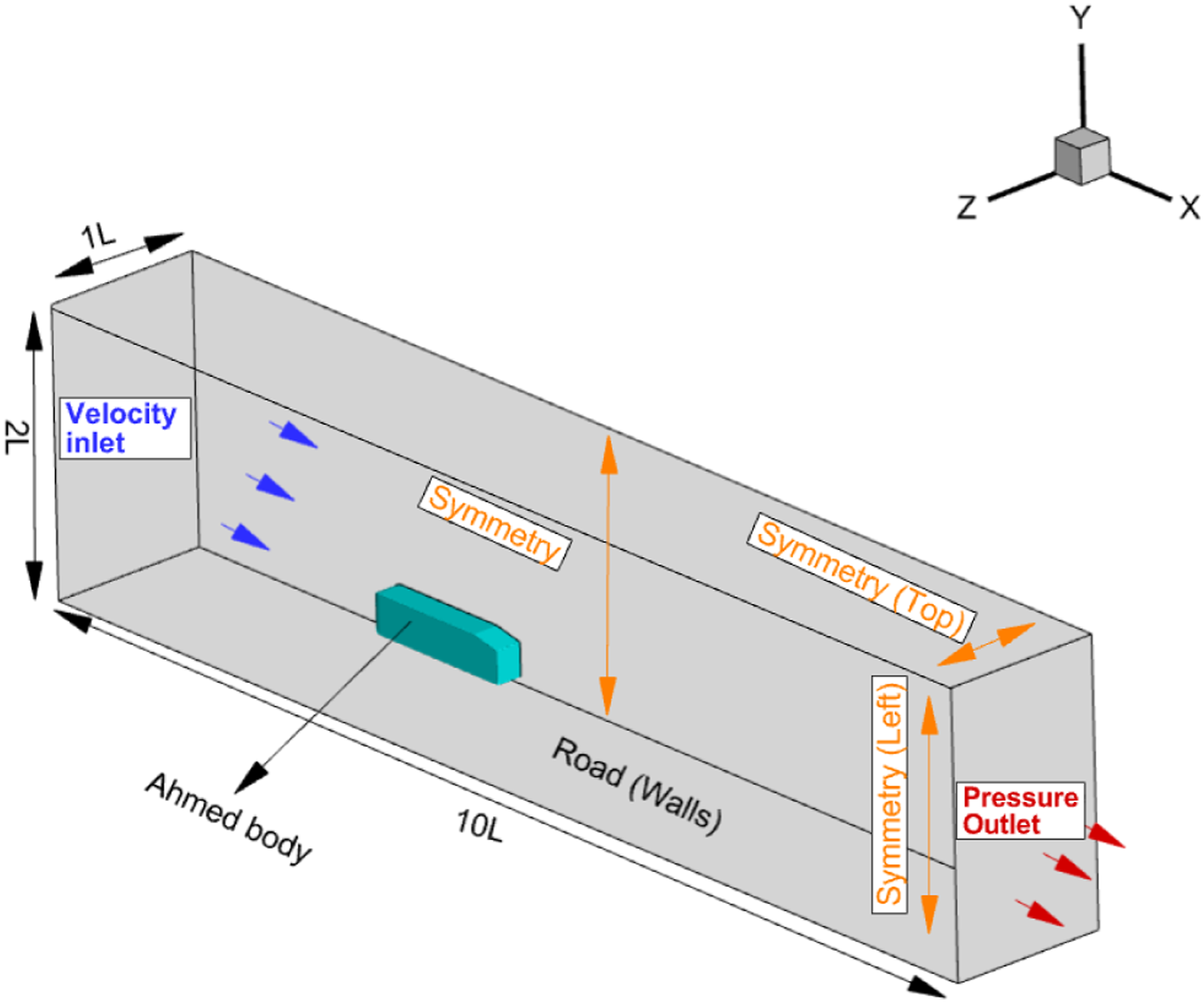

Figure 2 shows the domain setup of the Ahmed body, where the validation was performed with the experimental data and then replaced with the Araba body to be placed. Each case, that is, each parametric variation from Table 1, was performed, and a total of 108 model simulations were performed.

5. Mesh study

A mesh-independence study was conducted to assess the sensitivity of the drag coefficient to spatial discretization. Four progressively refined meshes, coarse, medium, fine, and very fine, were evaluated, each obtained through systematic refinement of the baseline grid. The baseline mesh was generated following standard meshing guidelines, with a far-field cell size of 1.25 m to reduce computational cost in regions of low turbulence intensity. Local mesh refinement and advanced sizing controls were applied in the near-body and wake regions to accurately capture key flow structures. Boundary layer resolution was ensured through the use of prism layers along the vehicle surfaces, with prism layer thickness selected to achieve appropriate wall-resolution (y+) values and ensure numerical convergence. For areas closer to the wall custom control is used. The grid-independent study, showing cases of the Richardson extrapolation approach, is presented in Table 2. This approach was performed using the procedure described by Celik et al.³³

Table 2.

Comparison table for mesh with different nodes and elements with C_d values.

Mesh	Cells	C_d Average
Mesh A	30625034	0.257
Mesh B	48331763	0.252
Mesh C	86581853	0.252
Mesh D	142550786	0.252

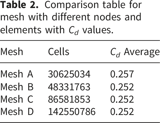
The total number of cells was 30, 48, 86 and 142 million cells in the coarse, medium, fine, and very fine meshes, respectively, resulting in the resolution presented in Table 2.

After the grid convergence study from Table 2, at mesh with 48 million cells was selected and simulations were performed. The mesh study was conducted for the model, which has the parameters of h=0.6m, h_d=0.6m, α=10°and R=0.3m. Figure 3 shows the mesh used in the study of the Araba body. However, the mesh is highly dense in the Araba region, front of the leading edge, and back of the trailing edge. To create a good quality mesh, factors such as orthogonal quality and skewness are considered. The trimmed Cell Mesher with Prism Layers are used. The chosen base size is 1.25 m for the least crucial areas of the domain with the cell size being less than 0.001 m for the rear area, this is achieved with the use of volumetric controls. The number of prism layers is set at 10 and the prism layer stretching is set at 1.1. An average orthogonal quality of 0.97183 was obtained which is considered to be the best orthogonal quality of 0.95 to 1 is taken in consideration. An average skewness of approximately about 8.8638 e-002 was obtained, and the best quality range for the skewness factor was 0 to 0.25. Then, the naming conditions were determined and a computational analysis was carried out.

Figure 3.

Araba body mesh.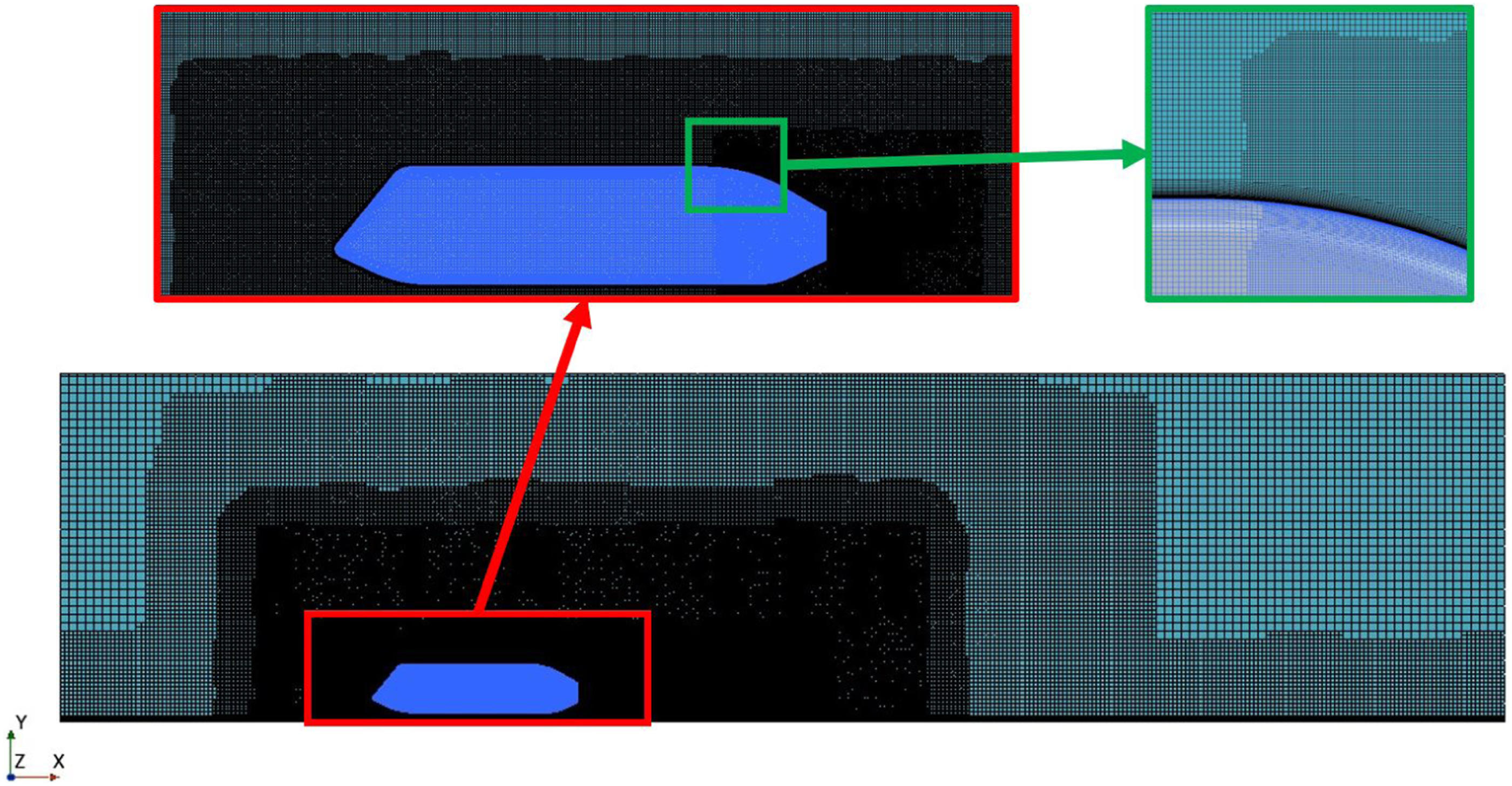

6. Validation of ahmed body

Validation of the Araba body was performed with the existing Ahmed body in comparison with the experimental analysis provided by Bayraktar et al.³⁴ Therefore, the validation was done with the scales Ahmed body that meets the dimensions of the Araba body. The Araba body was positioned with the rear of the Ahmed body located at the exact same points which helped validate the mesh and domain setup. The data obtained from the computational simulations were in good agreement with the experimental values. Figure 4, shows the validation of the experimental and simulation results. Figure 4(a) shows the results at 0°, 12.5° and 25°. In for the Figure 4 (b) the slant angles with the drag coefficient are obtained. As mentioned in “Turbulence model,” the accuracy of the results will depend highly on the turbulent model coefficients which have been used for the different slant angles.

Figure 4.

Experimental validation of the ahmed body. (a) Coefficient of pressure validation. (b)Pressure component of the drag validation.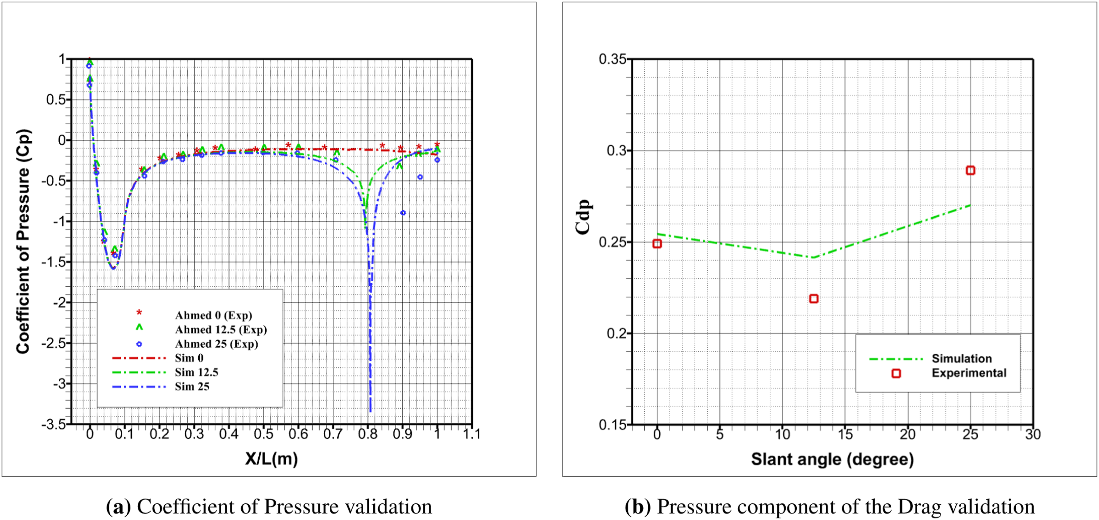

Validation was performed for both the Coefficient of Pressure and the Drag Coefficient of the Pressure, and it was concluded that the simulation setup was successfully validated for the experimental setup, and the other simulations were carried out.

Various turbulence models were tested for the simulations in the Araba body to compare the vortices in the rear region. All the turbulence models predicted the center location of the vortices quite well, but the dispersion lead to a deficiency in the flow separation. In Figure 5(a) for model 46, the comparison of the turbulence models shows that the k-ω DDES moved farther away, whereas the closer ranges are found for the k-ω SST and Wale LES models. In Figure 5(b) for model 108, the k-ω SST moves farther away than the other two models. For the model 108, the least drag value is obtained compared to the other models.

Figure 5.

Turbulence model comparison. (a) Vortex comparison with different turbulence models for model 46. (b) Vortex comparison with different turbulence models for model 108.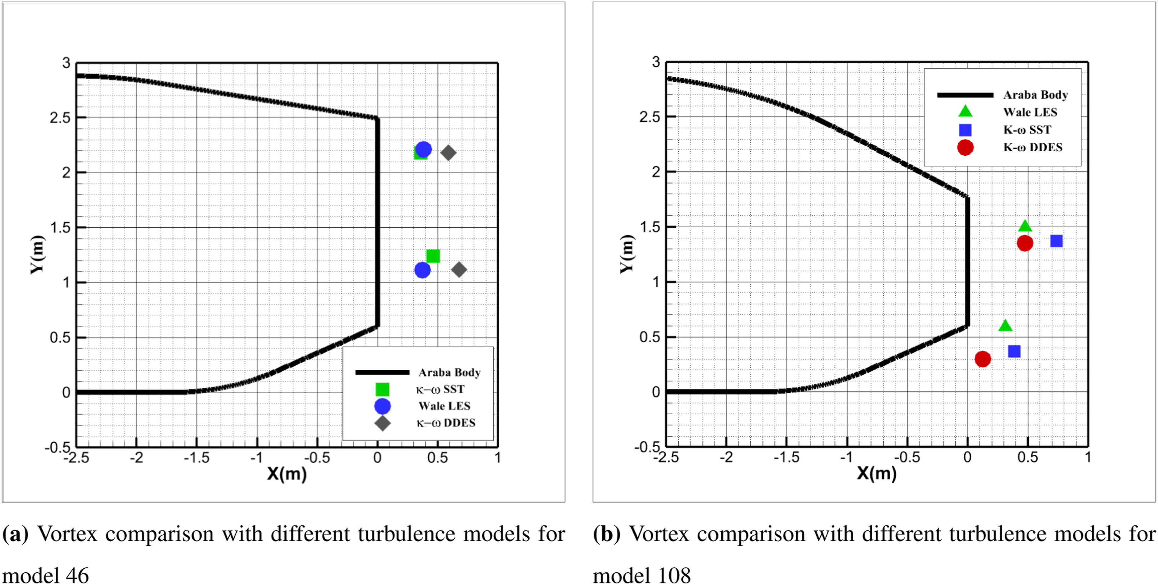

In Table 3, details metrics of the (C_d) and (C_dp) are mentioned with all three turbulent models for the highest drag model and the lowest drag model.

Table 3.

Comparison table for mesh with different nodes and elements with C_d values.

Model	Turbulent model	(C_d)	(C_dp)	Front height [m]	Roof rear angle [°]	Diffusor height [m]	Rounding radius [m]
46	SST	0.502272	0.458278	0.6	10	0.6	0
	DDES	0.454977	0.411964	0.6	10	0.6	0
	LES	0.495861	0.461665	0.6	10	0.6	0
108	SST	0.153695	0.113450	0.8	30	0.6	0.3
	DDES	0.167867	0.127855	0.8	30	0.6	0.3
	LES	0.149003	0.117284	0.8	30	0.6	0.3

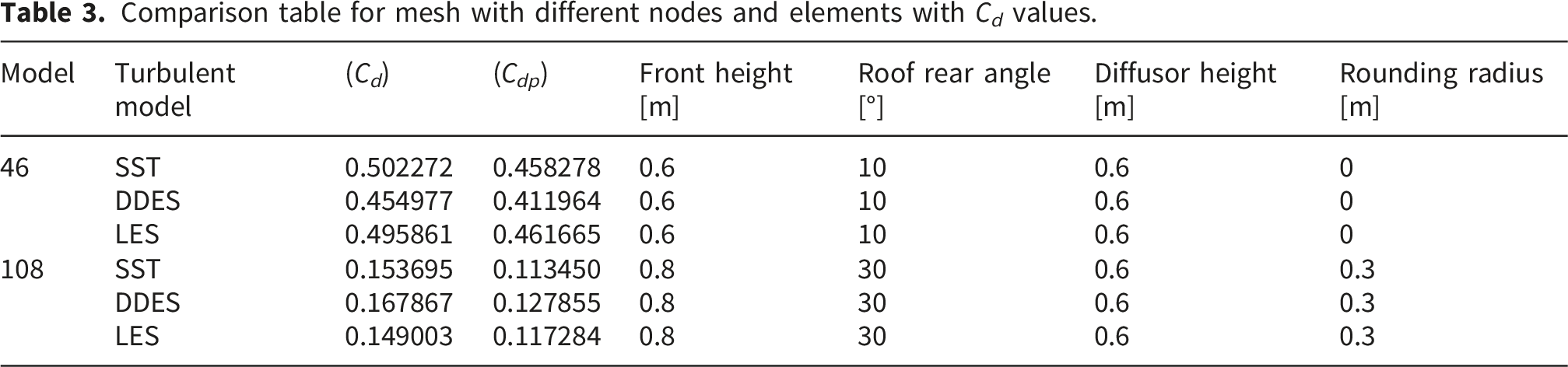
The discrepancies between the numerical simulations and experimental measurements, which become associated at large rear slant angles, are primarily associated with the transition to a fully separated and highly three dimensional wake regime. At these slant angles, the flow is governed by unsteady shear layer, intermittent de-attachment on the slanted surface, and large-scale vortex interactions in the rear wake. Such features are not fully resolved by steady or time-averaged RANS formulations leading to inaccuracies in the predicted pressure distribution and, consequently, in the drag coefficient. Numerical resolution further contributes to the observed discrepancies. Accurate prediction of large-slant-angle flows requires fine spatial and temporal resolution to resolve separated shear layers. Insufficient grid density, particularly in the near-wake and separation regions, or excessive numerical dissipation can suppress unsteady flow dynamics and bias time-averaged force predictions. In addition, achieving statistically converged solutions is more challenging for these strongly unsteady cases, increasing uncertainty in the computed mean quantities. A detailed comparison of different turbulent models for the pressure coefficient is presented in Appendix B. It´s known from previous studies that as the slant angle increases the discrepancies between the different models are more noticeable as the flow separates entirely from the rear surface.

Three different turbulent models were chosen and analyzed by comparing them with each other, as follows: k-ω SST (RANS): It is generally the most reliable and cost-effective option, offering strong near-wall and boundary-layer predictions. It is often used as the default starting point in many engineering simulations. WALE LES: This model has the highest level of physical accuracy as it directly resolves the large turbulent structures and unsteady vortices, especially in complex or transient flows. However, this improved fidelity comes with a much higher computational cost. k-ω DDES (hybrid): This model serves as a practical middle ground between the two. It behaves like a RANS model near the walls and switches to LES in separated regions, which improves accuracy compared to SST while remaining significantly less expensive than a full LES. LES has been proven to be more capable of resolving complex turbulent flows, allowing for results that closely match the experimental data being this a key point in this work. Hence LES model is chosen for the final simulations.

7. Computational study

The computations were performed using STAR CCM+ with HPC cluster ARINA. The chosen turbulence model for all the simulations was LES and they were performed with 800 CPU´s and 2 H100 Nvidia GPUs.

7.1. Mean velocity at planar section

First, with differences in the rounding radii of 0 m, 0.1 m and 0.3 m, respectively. For each of them, the velocity streamlines on 3 different X positions were analyzed being X1 = 0.5 m, X2 = 4 m and X3 = 8.13 m. In Figure 6, complete images of the vortices obtained are presented in detail. For the plane position X1, in the first case, that is R=0 m in Figure 6(A), the flow is highly turbulent with several vortices located on the upper part of the surface. For 0.1 rounding i. e Figure 6(E), another vortex is located in the lower part that is only visible in this case. For the case of 0.3 m i. e Figure 6(H), the vortices do not appear, meaning that the flow is going past the body without interference.

Figure 6.

Velocity contours for vortexes obtained in the YZ plane for the three different rounding cases for X1, X2 and X3. (A) X1 for R=0 m rounding. (B) X2 for R=0 m rounding. (C) X3 for R=0 m rounding. (E) X1 for R=0.1 m rounding. (F) X2 for R=0.1 m rounding. (G) X3 for R=0.1 m rounding. (H) X1 for R=0.3 m rounding. (I) X2 for R=0.3 m rounding. (J) X3 for R=0.3 m rounding.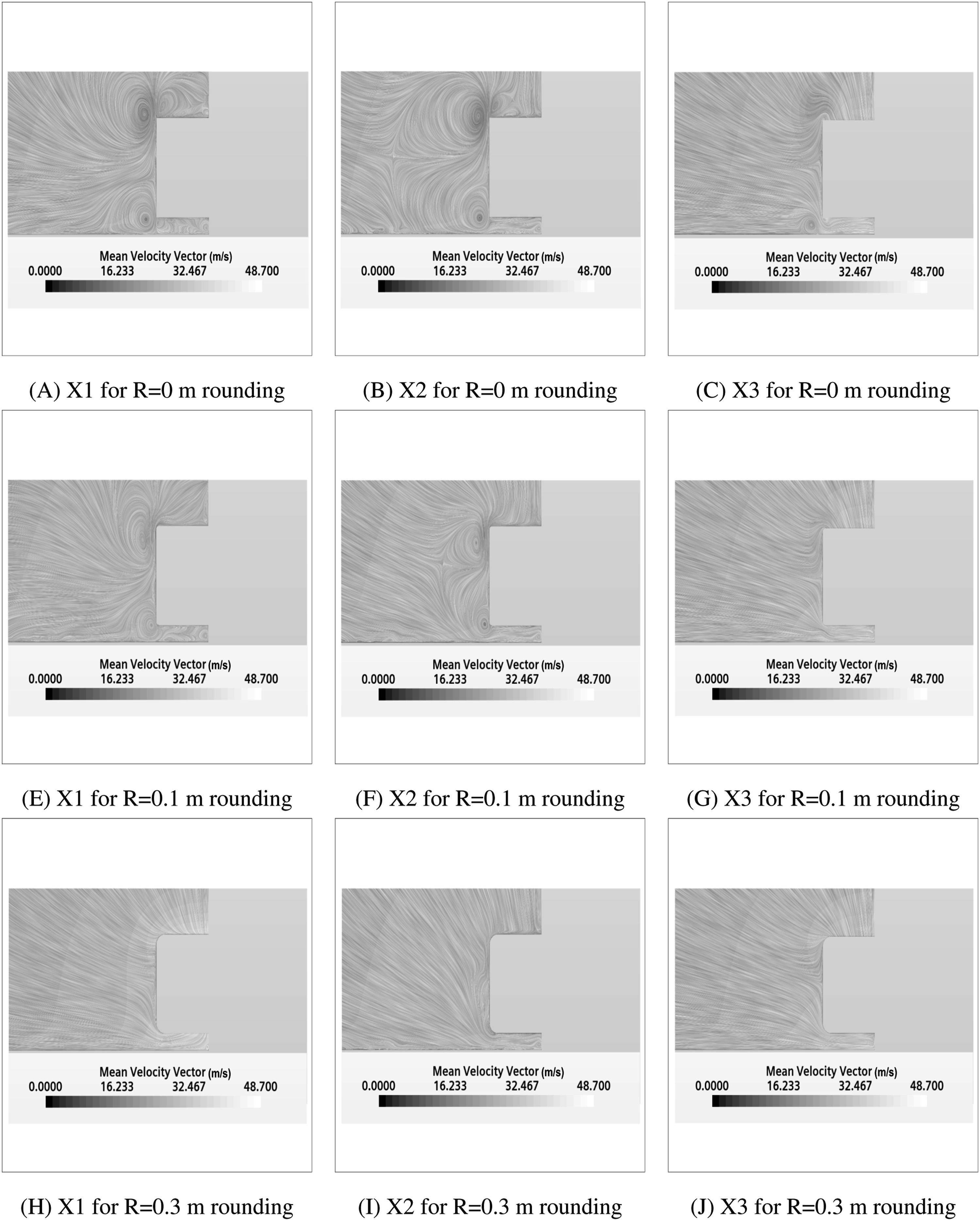

For the plane position X2, as the flow continues forward shown in Figure 6(B) and (F) it can be seen than in the first case for R = 0 m, there is a substantial change on the flow caused by the separation from the body. In the 0.3 m shown in Figure 6(I) there were small vortexes on the side of the body.

For plane position X3, as the flow reaches the rear of the vehicle, it is completely separated from the body in the case with no rounding. The velocity contours for this are shown in Figure 6(C), (G) and (J).

The wake acts both as the mean drag and as the downstream memory of of the vehicle, vortex-shedding and subsequent pairing or merger generate large-scale wake meandering that feeds back into the pressure field through convective re-encounters with the near region specifically for the low velocity. Cross correlation of surface pressure and wake probe signals will typically show a systematic phase lag equal to the convection time. Spatially, tip and root vortices create long-lived low-pressure cores in the near wake that increase induced pressure drag and, if asymmetric, introduce mean rolling/yawing moments — even when mean geometry is symmetric. The effects of the Reynolds number and the boundary layer having a direct impact to the shear layer, for both the transitional or for the laminar separation making the formation of the vortex locations, whereas for the fully turbulent separation makes the broadband high frequency energies.

7.2. Mean velocity for rounding variation

The analysis of the variation in the rounding radius shows how the vortices are obtained in change in the measurement with the increase in the radius, and the flow is passed without any interruption. For the variation for the R=0 m (Figure 7(a)), 0.1 m (Figure 7(b)) and 0.3 m (Figure 7(c)) are shown in the Figure 7. In Figure 7(a) and (b), twin vortices are obtained; in Figure 7(c) both vortices are dissipated.

Figure 7.

Variation in rounding radius R = 0 m, 0.1 m and 0.3 m. (a) Mean velocity vector at 0 m. (b) Mean velocity vector at 0.1 m. (c) Mean velocity vector at 0.3 m.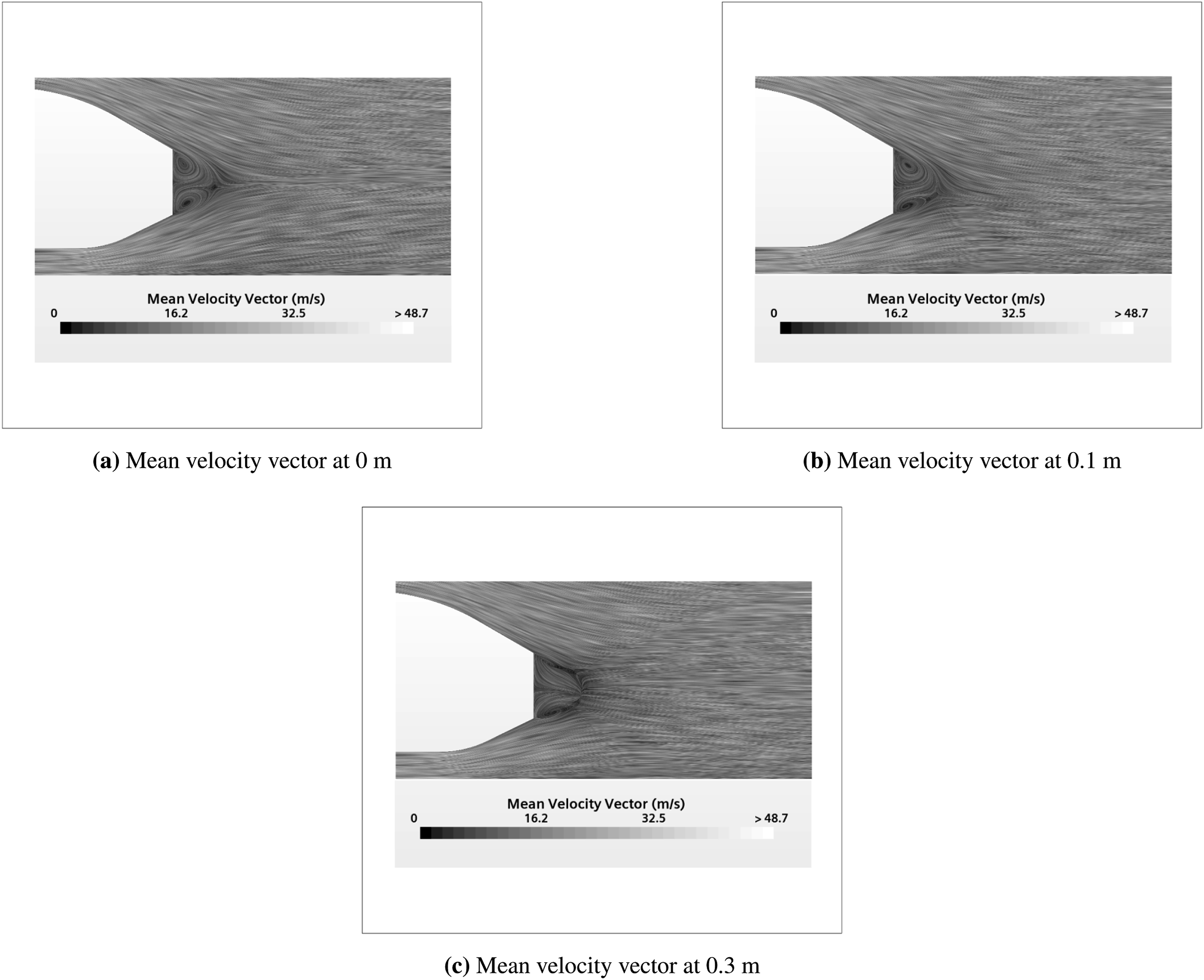

7.3. Mean velocity for slant angle variations

For the variations in the slant angles, that is α = 10°, 20°, and 30° the variations in the vortices are obtained and the results are presented in Figure 8. Looking at the rear wake, it can be seen that in Figure 8(a), there are two distinct vortices, as in the case with no rounding radius. In this case, the reverse flow vortex was larger, creating a larger low-velocity area on the rear wake. In Figure 8(b), in the case of the lower rear angle, a vortex is formed on the rear wake, which means that there is a low-velocity area. In the case with 20° the vortex is much smaller, and it disappears completely for the last case with 30° in Figure 8(c), indicating that there is no low-velocity area on the rear wake.

Figure 8.

Variation in slant angle. (a) Mean velocity vector for 10°. (b) Mean velocity vector for 20°. (c) Mean velocity vector for 30°.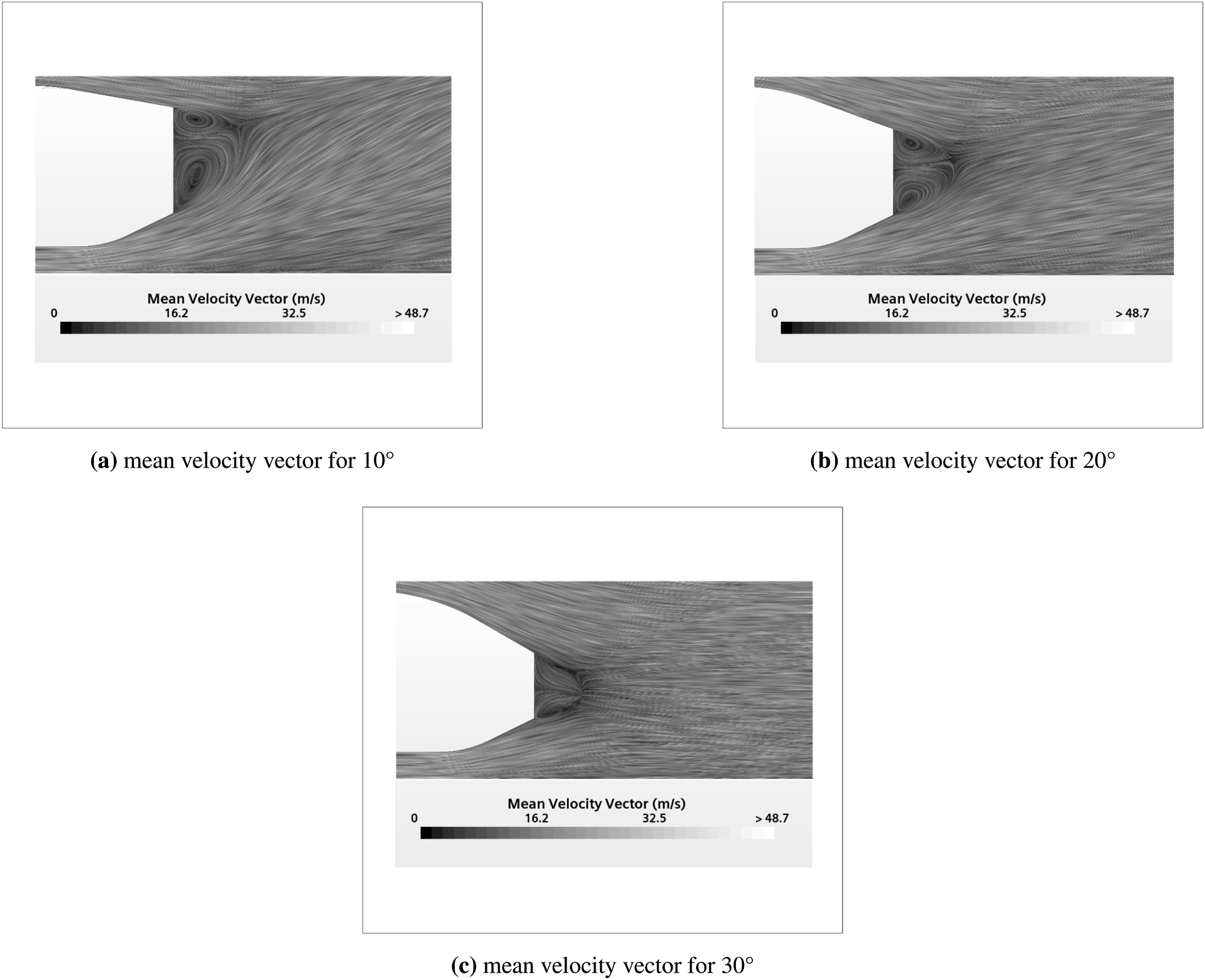

7.4. Mean velocity for various diffuser heights

The variations in diffuser height h_d = 0 (i.e no diffuser), 0.2m, 0.4m, and 0.6m. Figure 9 shows a representation of the diffuser height variation for the Araba body. It can be seen than in the first case with no diffuser, the downwards flow encloses the flow current that comes from the underside and causes the low velocity area to contact the floor, creating high amounts of drag, which is shown in Figure 9(a). In the next case, although the recirculation area is in contact with the floor, the area itself is much smaller as the flow is pushed upwards by the small diffuser, as shown in Figure 9(b). For the 0.4 m and 0.6 m shown in Figure 9(c) and 9(d) the low velocity area did not touch the floor region. It is possible to appreciate a much more turbulent flow in the first case as the flow travels inward into the body, in contrast with the other case in which the flow goes almost straight and does not generate any turbulence. This is a consequence of the downwards traveling flow, in the case with no diffuser, which does not encounter any opposition as it travels downwards toward the ground.

Figure 9.

Variation in diffuser height. (a) Mean Velocity Vector for no diffuser. (b)Mean Velocity Vector for 0.2 diffuser. (c)Mean Velocity Vector for 0.4 diffuser. (d)Mean Velocity Vector for 0.6 diffuser.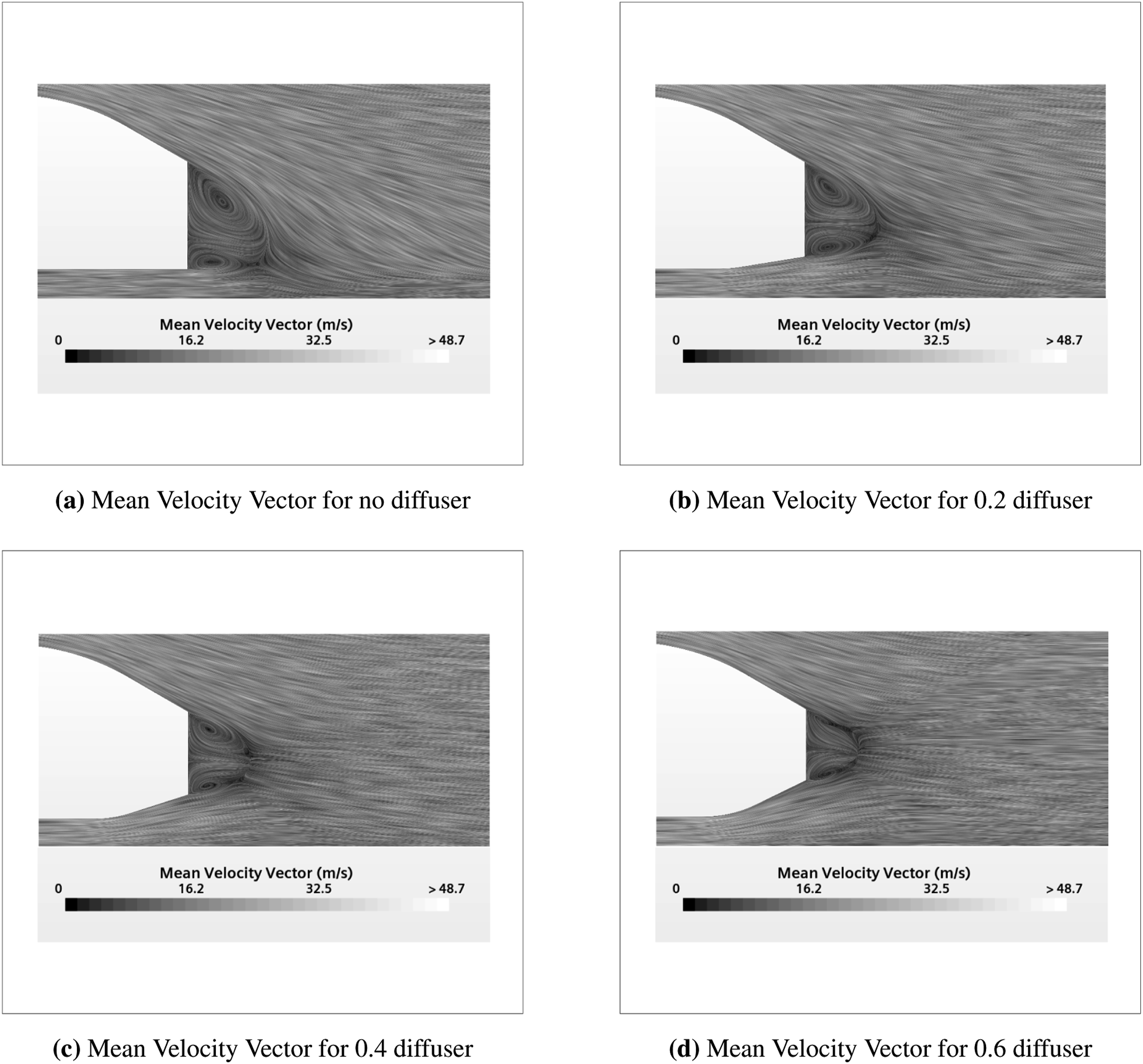

However, for all of the above cases the vortices can be seen and dissipate in the higher cases for the variations; however, for the frontal height (H) variations, no vortex is generated is worth mentioning.

The objective of this work is to assess the aerodynamic drag characteristics of a vehicle using a geometrically simplified configuration suitable for CFD analysis. In line with established Ahmed body–based validation approaches, minor appendages and wheels are omitted to reduce geometric complexity and numerical uncertainty while preserving the dominant flow features governing drag. A stationary ground plane is employed for the same reason, as the primary drag mechanisms of interest are not expected to be significantly influenced by ground motion under the present conditions.

8. Surface shear stress

Surface mean shear stress contributes to skin-friction drag, which does not have drastic effects on drag for bluff vehicles but can have more significant effects on the stream line designs. Mean shear stress also offers information on boundary-layer state and separation behavior, making it a notable metric for determining drag sources and flow control efficacy. In Figure 10, the mean of shear stress is described for both the high drag coefficient model and the low drag coefficient model in comparison with all three turbulent models taken into consideration. Figure 10(a)–(c) shows the model with higher drag with different turbulence models and Figure 10(d)–(f) shows the model with lower drag with different turbulence models.

Figure 10.

Representation of the mean shear stress for the high drag coefficient model and low drag coefficient model. (a) k-ω SST. (b)k-ω DDES. (c) LES. (d) k-ω SST. (e) k-ω. (f) k-ω.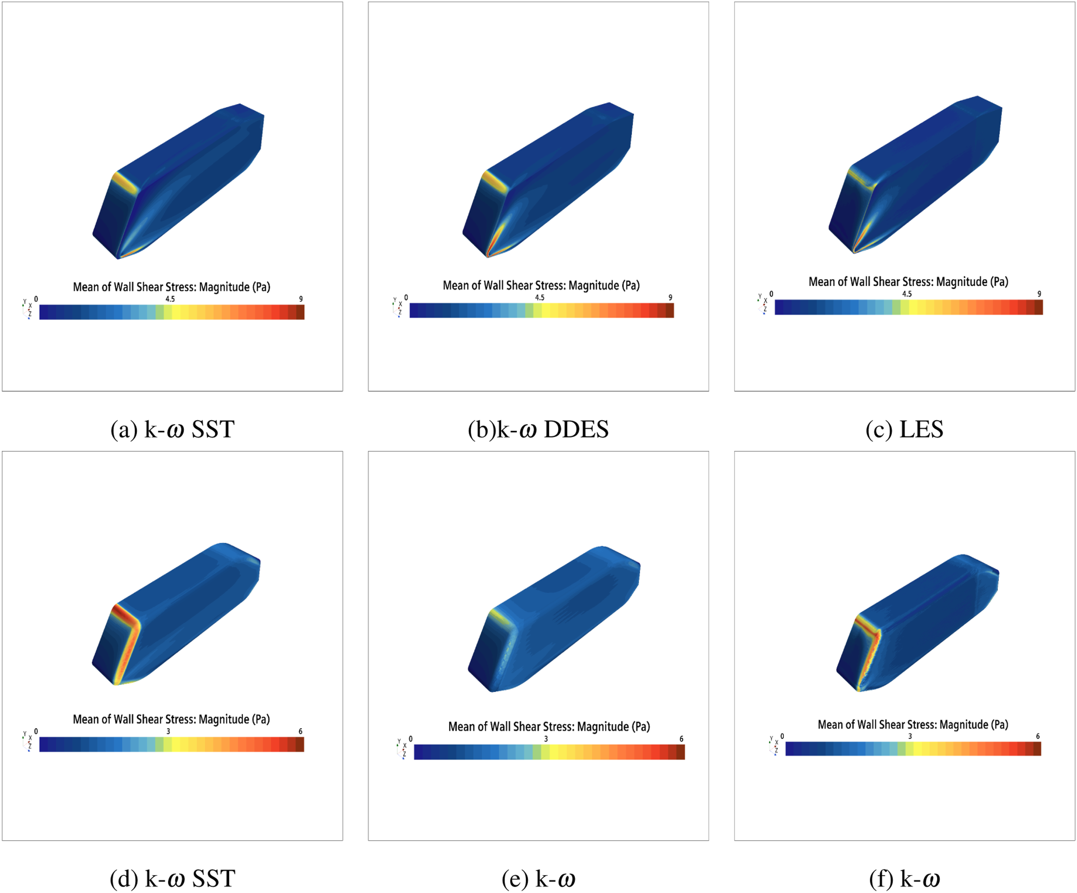

9. Drag based results

The effects of the Drag Coefficient and Coefficient of Drag Pressure are shown in Figure 11. The rounding radius (R) has an impact on the drag coefficient as the data shows a 2.5% drag reduction for both (C_d) and (C_dp) between the 0 and 0.3 m, as case shown in Figure 11(a). The results obtained show the improvement of the diffuser even for smaller heights as the difference on the drag value is much bigger from 0 to 0.2 that between other configurations so this shows that any type of diffuser is a positive difference on the aerodynamics of the body shown in the Figure 11(b). In this case, the drag does not follow a downwards curve, as in the other cases, and the value of the 0.4 m height is better than that one with 0.8 m height shown in Figure 11(c). The drag reduction almost follows a perfect line between the values meaning that there is a possibility of decreasing the drag value even more when using a higher rounding radius, but this is not part of this study. In the graph, it can be seen that the higher the rear angle, the lower the drag value, as shown in Figure 11(d). LES is the main turbulence model for all the main simulations that are run, and the graphs are represented through it.

Figure 11.

Graphical representations for all the varying parameters a) R= 0 m, 0.1 m and 0.3, b) h_d = 0.2 m, 0.4 m, 0.6 m and 0.8 m, c) H = 0.4 m, 0.6 m and 0.8 m d) α = 10°, 20° and 30°.(a) Effects of frontal rounding (R). (b) Effects of variation in diffuser (h_d). (c) Effects of variation in frontal height (H). (d) Effects of variation in slant angle (α).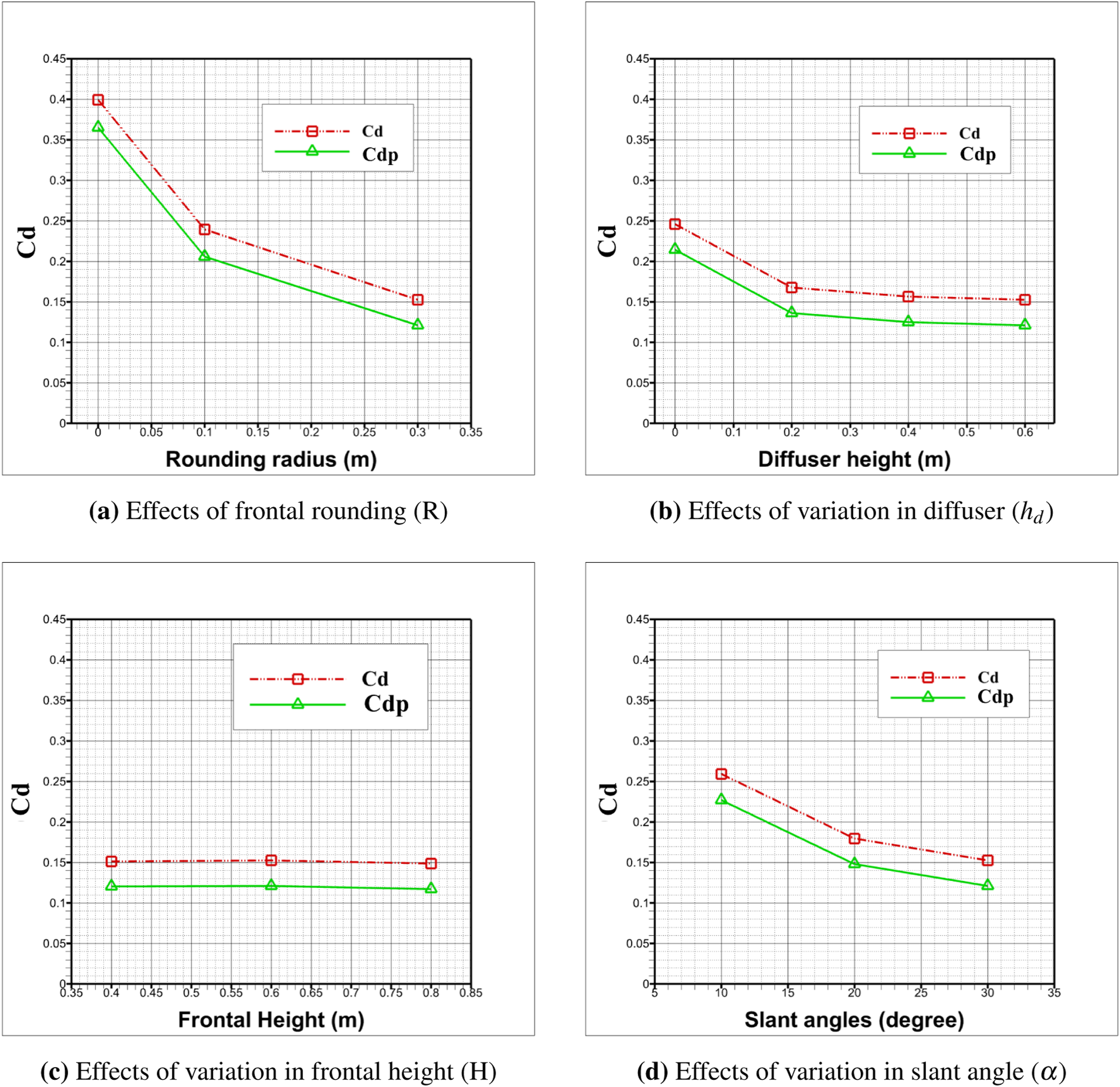

In the first part of the study, 3 D graphs of the data were created using MATLAB to determine the combined effects of the parameters on the Drag Coefficient. The first four graphs were for the diffuser height and the next three were used for the three rounding radii, which are shown in Figure 12.

Figure 12.

3D graphs off the effects of rounding and diffuser heights on Drag Coefficient. (a) No Diffuser. (b) Diffuser with 0.2 m. (c) Diffuser with 0.4 m. (d) Diffuser with 0.6 m. (e) 0 m rounding. (f) 0.1 m rounding. (g) 0.3 m rounding.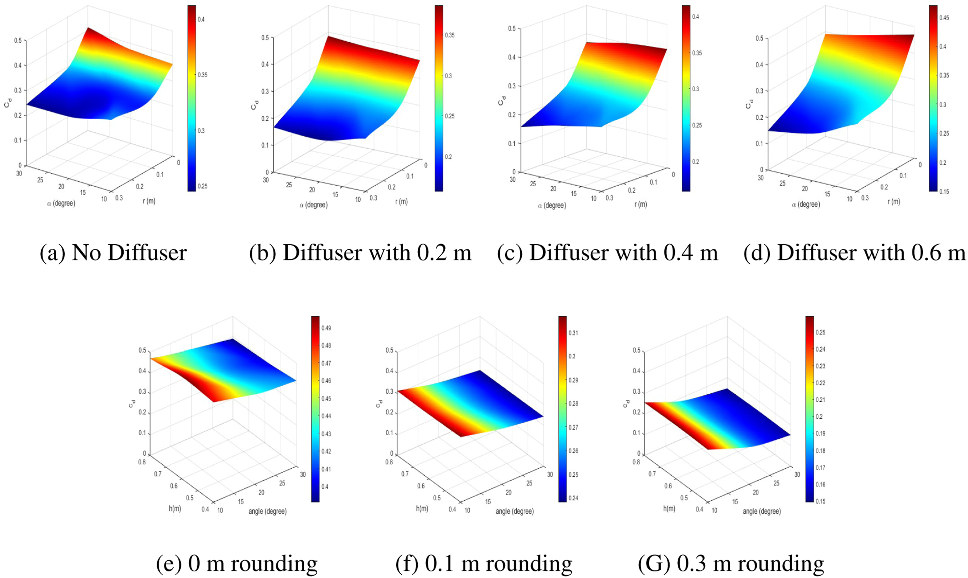

The slant angle against the rounding radius for each diffuser height is plotted. In this case, the front height was fixed at 0.8 m as in the previous graphs, it was determined that it does not produce a significant difference. This follows the conclusions of Ahmed et al.¹ who postulated that the drag coefficient on the front only amounted to an 8% difference. For the no-diffuser case shown in Figure 12(a), there is a large difference compared to the previous case, as it is seen that when the slant angle is increased, the drag is higher for the cases with no rounding. For the 0.2 m shown in Figure 12(b), there is a much larger difference obtained by changing the rounding radius, especially for a higher slant angle. For the 0.4 m shown in Figure 12(c) it is noted that increasing the slant angle positively affects the drag in all the cases and that at the same time, the rounding radius effect is much more notable than in any of the previous cases. For the 0.6 m, as shown in Figure 12(d), it is possible to find the best and worst Drag Coefficients as the case with no rounding radius and 10° angle experience the largest drag values and at the same time, the case with 0.3 m radius and 30° slant angle has the lowest Drag Coefficient. To conclude, it can be determined that the major drag generator is the rounding radius and that the smallest drag changes are produced by the front height. In the following section, a more thorough analysis of the flow will be carried out to further explain the results obtained.

For the rounding radius the graphs 12(e–g), the diffuser height is fixed on a value of 0.6 m and the rounding radius was changed between the graphs. The case with no rounding radius is shown in Figure 12(e). From the results, it is seen that independent of the other two variables, the drag obtained is higher than 0.35, and that it is never going upwards of 0.5. Looking at the other variables it´s possible to see that their higher drag values are obtained with a front height of 0.6 m although the height by itself is not producing a big difference. The main change appreciated is the slant angle with a difference of close to 0.1 between the 10° and 30° cases. The maximum Drag Coefficient obtained is almost 0.2 times lower than the maximum value obtained with the previous parameter. It is also seen that the shape is much more linear and that for example there is no bulge for the 0.6 m front height as shown in Figure 12(f). Lastly, the case with a rounding radius of 0.3 m is plotted and analyzed. On this case it´s where the lowest Drag Values have been obtained with the best case scenario being 30°, 0.8 m height and 0.6 m diffuser. At the same time, a major difference in the slant angle compared with the other cases can be seen, as shown in Figure 12 (g).

For the purposes of CFD validation, the Drag Coefficient is decomposed into pressure and skin-friction components. In agreement with established experimental and numerical studies of bluff automotive geometries, pressure drag accounts for approximately 85% of the total drag. The predicted skin-friction contribution exhibits limited sensitivity to the investigated configurations, fluctuating around a value of 0.031 and representing, on average, 14% of the total drag. This behavior is attributed to the concentration of peak wall shear stress in the frontal region of the vehicle, where the boundary layer remains largely unaffected by geometric modifications, with the exception of variations in bumper height. The consistency of the shear-drag contribution across cases provides additional confidence in the robustness of the CFD predictions.

10. Conclusion

In this study, a detailed research work is carried out for the Araba body: first, experimental validation is performed with the Ahmed body itself, then with all the different parameters; various cases of 108 geometries were created, and simulations were performed. The (C_d) and (C_dp) values were obtained from all the simulated geometries. An evaluation of the parameter that has a higher influence on the reduction of drag and surface generation. The design with higher parameters combined had the lowest drag value. After studying the heavy vehicle in all its configurations, it is possible to determine that the best configurations on the Araba body have a better drag value for heavy vehicles although further studies are required to validate this. This work utilized of LES simulations for commercial vehicles, especially passenger vehicles. At the same time the results obtained were wakes and vortexes. On the simulations itself it was determined that the most important parameter is the rounding radius concluding that the best drag values were obtained with 0.3 m radius, obtaining values as lower as 0.149 drag. Other crucial parameters were the slant angle, which could reduce the drag by up to 40%. In cases with no rounding radius, increasing the slant angle might create more drag. This leads to the conclusion that the rounding radius impact on the slant angle needs to be further studied, as it appears that changes produced by it are sufficiently significant. The diffuser height was found to have a significant effect on the drag, especially between the cases of no diffuser and a 0.2 m diffuser. Larger diffuser heights obtained only marginally better drag when using a slant angle of 30° and a rounding radius of 0.3 m. Lastly, the last parameter studied was the front height which was the one that produced the least impact on the Drag Coefficient, although the flow difference in the diffuser may indicate that further improvements of the front area can create higher differences on the drag. Keeping the fact that the parameters cannot be varied much more, as the shape of the vehicle would change too much and would not be realistic, as this model is designed with the intention of being the template for new bus bodies, there are some cases in which even though they have a much smaller Drag Coefficient, they are not as economically viable as the internal space is reduced. For further studies, a more thorough analysis of the flow in the most relevant case, along with an exclusive setup of the Araba body, is being conducted to perform the experimental validation for the aerodynamic analysis in a larger wind tunnel. The Araba body is considered a heavy reference vehicle, considering various conditions. The dimension of the design has a total length of 12140 mm, with a total height of 2880 mm, considering a standard commercial bus dimension. Another important factor is that sustainable propulsion solutions, such as batteries and hydrogen power, adds weight to the design which can reduce the efficiency of the vehicle requiring a more aerodynamic design to create a drag reduction and even improving the performance.

Footnotes

Acknowledgments

The authors are grateful for the support provided by SGIker of UPV/EHU.

ORCID iDs

Vivekamanickam Koothan-Venkateswaran

Koldo Portal-Porras

Unai Fernandez-Gamiz

Author contributions

Roberto Garcia-Fernandez: Conceptualization (lead), data curation (lead), formal analysis (equal), investigation (lead), and methodology (equal).

Vivekamanickam Koothan-Venkateswaran: Conceptualization (equal), data curation (equal), methodology (equal), resources (equal), writing – original draft (lead), and software (equal).

Imanol Urruchi-Gavina: Conceptualization (equal), data curation (equal), methodology (equal), resources (equal), writing – original draft (equal), and software (equal).

Koldo Portal-Porras: Conceptualization (equal), data curation (equal), funding acquisition (lead), methodology (equal), project administration (equal), supervision (equal), and validation (equal)

Unai Fernandez-Gamiz: Conceptualization (equal), data curation (equal), formal analysis (equal), funding acquisition (equal), investigation (equal), supervision (lead), and validation (lead).

Funding

The authors disclosed receipt of the following financial support for the research, authorship, and/or publication of this article: This research was support by the Government of the Basque Country: DBaskIN and ELKARTEK24/78; and CIEMAT: Energía eólica offshore para el ensayo y el desarrollo energético de energías renovables e hidrógeno verde; The work of U.F.G. was partially supported by Government of the Basque Country: ITSAS-REM (IT1514-22).The authors appreciate the support of the Navarre government through the AEROSUN research program.

Declaration of conflicting interests

The authors declared no potential conflicts of interest with respect to the research, authorship, and/or publication of this article.

Data Availability Statement

All data generated/analyzed in the study are included in the manuscript. Supplementary data associated with this article can be found in the online version, at Zenodo ().³⁵

Appendix

References

Syed

Ramm

Faltin

. Some salient features of the time-averaged ground vehicle wake. SAE Transactions, 1984, pp. 473–503.

Tunay

Sahin

Ozbolat

. Effects of rear slant angles on ahmed body flow characteristics. Experimental Thermal and Fluid Science 2014; 57: 165–176. https://doi.org/10.1016/j.expthermflusci.2014.04.016

Tunay

Yaniktepe

Sahin

. Computational and experimental investigations of vortical flow structures in the near wake region downstream of the ahmed vehicle model. Journal of Wind Engineering and Industrial Aerodynamics 2016; 159: 48–64. https://doi.org/10.1016/j.jweia.2016.10.006

Barros

Bore

Noack

, et al. Bluff body drag manipulation using pulsed jets and the coanda effect. Journal of Fluid Mechanics 2016; 805: 422–459.

Barros

Bore

Noack

. Spohn. Resonances at the forced turbulent wake past a 3d blunt body. Physics of Fluids 2016; 28(6).

Rao

Minelli

Basara

, et al. On the two flow states in the wake of a hatchback ahmed body. Journal of Wind Engineering and Industrial Aerodynamics 2018; 173: 262–278. https://doi.org/10.1016/j.jweia.2017.10.021

Guilmineau

Deng

Leroyer

, et al. Assessment of hybrid rans les formulations for flow simulation around a ahmed body. Computers and Fluids 2018; 176: 302–319. https://doi.org/10.1016/j.compfluid.2017.01.005

Grandemange

Cadot

Gohlke

. Reflectional symmetry breaking of separated flow over three-dimensional bluff bodies. Phys. Rev. E 2012; 86: 035302. https://doi.org/10.1103/PhysRevE.86.035302

Grandemange

Cadot

Courbois

, et al. A study of wake effects on the drag of ahmed’s squareback model at an industrial scale. Journal of Wind Engineering and Industrial Aerodynamics 2015; 145: 282–291. https://doi.org/10.1016/j.jweia.2015.03.004

10.

Volpe

Devinant

Kourta

. Unsteady experimental characterization of natural wake of squareback-ahmed model. ASME AMERICAN SOCIETY OF MECHANICAL ENGINEER 2014; 1C: 1–9.

11.

Fan

Xia

Chu

, et al. Experimental and numerical analysis of the bi-stable turbulent wake of a rectangular flat-backed bluff body. Physics of Fluids 2020; 32(10): 105111. https://doi.org/10.1063/5.0019794

12.

Grandemange

Gohlke

Cadot

. Bi-stability in turbulent wake past parallelepiped bodies with various aspect ratios and wall effects. Physics of Fluids 2013; 25: 5103.

13.

Bonnavion

Cadot

. Unstable wake dynamics of rectangular flat-backed bluff bodies with inclination and ground proximity. Journal of Fluid Mechanics 2018; 854: 196–232. https://doi.org/10.1017/jfm.2018.630

14.

Haffner

Borée

Spohn

, et al. Mechanics of bluff body drag reduction during transient near-wake reversals. Journal of Fluid Mechanics 2020; 894: A14. https://doi.org/10.1017/jfm.2020.275

15.

Khalighi

Chen

K-H

Iaccarino

. Unsteady aerodynamic flow investigation around a simplified square-back road vehicle with drag reduction devices. Journal of Fluids Engineering 05 2012; 134(6): 061101. https://doi.org/10.1115/1.4006643

16.

Kang

Essel

Roussinova

, et al. Effects of approach flow conditions on the unsteady three-dimensional wake structure of a square-back ahmed body. Phys. Rev. Fluids 2021; 6: 034613. https://doi.org/10.1103/physrevfluids.6.034613

17.

Hesse

Morgans

. Simulation of wake bimodality behind squareback bluff-bodies using les. Computers and Fluids 2021; 223: 104901. https://doi.org/10.1016/j.compfluid.2021.104901

18.

Delassaux

Mortazavi

Itam

, et al. Sensitivity analysis of hybrid methods for the flow around the ahmed body with application to passive control with rounded edges. Computers and Fluids 2021; 214: 104757. https://doi.org/10.1016/j.compfluid.2020.104757

19.

Buscariolo

Assi

GRS

Sherwin

. Computational study on an ahmed body equipped with simplified underbody diffuser. Journal of Wind Engineering and Industrial Aerodynamics 2021; 209: 104411. https://doi.org/10.1016/j.jweia.2020.104411

20.

Aguerre

Gimenez

Escribano

, et al. Aerodynamic study of a moving ahmed body by numerical simulation. Journal of Wind Engineering and Industrial Aerodynamics 2024; 245: 105635. https://doi.org/10.1016/j.jweia.2023.105635

21.

Naseeb

Agelin-Chaab

. Flow features of the ahmed body at a low reynolds number. International Journal of Heat and Fluid Flow 2022; 98: 109052.

22.

Serre

Minguez

Pasquetti

, et al. Simulating the turbulent flow around the ahmed body: a french–german collaborative evaluation of les and des. Computers and Fluids 2013; 78: 10–23, LES of turbulence aeroacoustics and combustion. https://doi.org/10.1016/j.compfluid.2011.05.017

23.

Krajnovic

Davidson

. Numerical study of the flow around a bus-shaped body. Journal of Fluids Engineering 2003; 125(3): 500–509. https://doi.org/10.1115/1.1567305

24.

Aultman

Duan

. Analysis of flow past a double-slanted ahmed body. Fluids 2025; 10(2): 35. https://doi.org/10.3390/fluids10020035

25.

Naseeb

Agelin-Chaab

. Experimental investigation of the flow features around an elliptical Ahmed body. Physics of Fluids 2022; 34(10): 105119.

26.

Naseeb

Agelin-Chaab

. Investigation of the wake flow around the elliptical ahmed body using detached eddy simulation. International Journal of Heat and Fluid Flow 2023; 101: 109125.

27.

Garcia-Fernandez

Portal-Porras

Irigaray

, et al. Cnn-based flow field prediction for bus aerodynamics analysis. Scientific Reports 2023; 13(1): 21213. https://doi.org/10.1038/s41598-023-48419-4

28.

Pope

. Turbulent flows. Measurement Science and Technology 2001; 12(11): 2020–2021. https://doi.org/10.1088/0957-0233/12/11/705

29.

Fureby

Tabor

Weller

, et al. A comparative study of subgrid scale models in homogeneous isotropic turbulence. Physics of fluids 1997; 9(5): 1416–1429. https://doi.org/10.1063/1.869254

30.

Nicoud

Ducros

. Subgrid-scale stress modelling based on the square of the velocity gradient tensor. Flow, turbulence and Combustion 1999; 62(3): 183–200. https://doi.org/10.1023/a:1009995426001

31.

Draksler

Končar

Cizelj

, et al. Large eddy simulation of multiple impinging jets in hexagonal configuration–flow dynamics and heat transfer characteristics. International Journal of Heat and Mass Transfer 2017; 109: 16–27. https://doi.org/10.1016/j.ijheatmasstransfer.2017.01.080

32.

Ducros

Franck

Poinsot

. Wall-adapting local eddy-viscosity models for simulations in complex geometries. Numerical Methods for Fluid Dynamics VI 1998; 1–7.

33.

Celik

Ghia

Roach

. Procedure for estimation and reporting of uncertainty due to discretization in cfd applications. Journal of Fluids Engineering 2008; 130(7): 078001.

34.

Bayraktar

Landman

Baysal

. Experimental and computational investigation of ahmed body for ground vehicle aerodynamics. SAE Transactions 2001; 110: 321–331.

35.

University of the Basque Country . Araba Body. Zenodo, 2025. https://doi.org/10.5281/zenodo