Prediction of laser welding molten pool light intensity distribution based on an artificial neural network

Abstract

This study aims to develop a spatio-temporal predictive model for the luminous intensity distribution of the laser welding molten pool—a key visual indicator of process stability and quality—to overcome the limitations of conventional analytical models in handling complex multi-physical interactions. A data-driven framework based on a nonparametric artificial neural network architecture is proposed. Gaussian functions are employed as radial basis functions to capture localized spatio-temporal variations in the light field. The root mean square error is adopted as the evaluation metric and integrated into a systematic hyperparameter optimization procedure to enhance model fidelity and robustness. The optimized model successfully predicts two distinct molten pool luminous patterns under different welding conditions. Predictions show strong agreement with synchronized high-speed experimental images, confirming the model’s accuracy and generalization capability. This method effectively reconstructs the molten pool’s luminous signature, demonstrating significant potential for real-time process monitoring, online anomaly detection, and non-destructive quality assessment in advanced laser welding operations.

Keywords

laser welding molten pool artificial neural network machine vision nonparametric statistical model

Introduction

Laser welding has firmly established itself as a cornerstone technology in modern high-value manufacturing, prized for its precision, speed, and automation compatibility. Its adoption in sectors such as automotive,¹ aerospace,² and battery manufacturing is critical.³ However, the process’s extreme energy concentration and rapid thermal cycles make it uniquely susceptible to a range of defects that directly compromise product integrity.⁴ The most common and detrimental flaws include porosity (caused by keyhole instability or contamination), solidification cracking (due to thermal stress and vulnerable material composition), spatter (from violent metal vaporization), and incomplete penetration or melt pool instability. These defects are often stochastic, emerging from subtle, real-time interactions between process parameters, material properties, and joint conditions.⁵ A critical, yet complex, factor influencing this defect formation is the behavior of the process-induced plasma. In keyhole-mode welding, the formation of a plasma plume—a cloud of ionized metal vapor and shielding gas—above the workpiece exerts a dual and decisive influence on weld quality. Under controlled conditions, a stable, optically transparent plasma can enhance energy coupling to the keyhole and provide secondary shielding from atmospheric contamination.⁶ Conversely, a dense, over-developed, or unstable plasma acts as a primary defect driver. It absorbs, scatters, and defocuses the incident laser beam (plasma shielding), directly attenuating the energy delivered to the workpiece.⁷ This energy loss is a direct cause of incomplete penetration and shallow welds. Furthermore, plasma instability is intrinsically linked to keyhole instability; fluctuations in the plasma’s size, shape, and intensity often precede the collapse or oscillation of the keyhole, leading directly to the formation of porosity and excessive spatter.⁸ Therefore, the plasma’s state serves as a crucial real-time proxy for process health, where its undesirable behavior is both a symptom and a cause of the very defects that degrade weld quality.⁹ Traditional post-weld inspection methods are reactive and costly, incapable of preventing such defect formation.¹⁰ Therefore, the industrial imperative has shifted toward in-situ, real-time monitoring of key physical signatures, such as plasma emissions and molten pool radiation, to detect the process deviations that precede defect generation.¹¹ The optical emission from the molten pool and the plasma plume together form a rich, information-dense signal. Variations in their spatio-temporal intensity distribution are closely linked to the onset of specific defects.¹² Consequently, developing accurate models to predict and interpret these coupled optical signatures is fundamental to building an intelligent, defect-averse welding system. A robust predictive model can serve as a digital twin for real-time comparison, enabling the early detection of anomalies rooted in plasma or keyhole instability.¹³ This capability is the precursor to adaptive control,¹⁴ where parameters like laser power or speed can be adjusted in real-time to correct the process trajectory before a defect solidifies.^15,16 Recent studies have demonstrated the value of acquiring multi-physics information from the molten pool for improved process monitoring.¹⁷ A single-camera system capable of simultaneous measurement of 2D temperature and flow fields as well as local 3D molten pool information in additive manufacturing has been developed.¹⁷ Similarly, fusing visual features of the melt pool with temperature field data within an artificial neural network enabled penetration status detection in variable-groove welding with over 92% accuracy.¹⁸ These findings highlight the effectiveness of integrating optical signatures with neural network-based models for molten pool characterization.^17,18 A comprehensive review of in-situ optical monitoring in laser beam welding has highlighted the potential of combining optical signals with machine learning for effective process control.¹⁹ Meanwhile, the nonlinear effect of laser frequency modulation on molten pool width in deep penetration laser welding has been systematically investigated, revealing that frequency modulation can significantly alter molten pool geometry through complex thermal-fluid interactions.²⁰

In response to these challenges, this study proposes a novel spatiotemporal prediction framework for molten pool light intensity distribution in laser welding. The framework integrates a normalized radial basis function neural network (RBFNN) with nonparametric statistical methods—a methodological synergy not previously employed in this domain—to dynamically characterize the highly nonlinear optical-thermal-fluid coupling inherent to the welding process. Departing from conventional post-process monitoring or physics-based models constrained by simplifying assumptions, the proposed model achieves low-latency, high-accuracy prediction of intensity distributions directly from process parameters, enabling real-time closed-loop control without dependence on predefined physical formulations. The root mean square error is employed as the primary evaluation metric to quantitatively assess light-field prediction fidelity, providing an interpretable and standardized measure of model performance that directly supports hyperparameter optimization and cross-model comparison. By effectively bridging high-speed vision sensing with adaptive process control, this framework represents a significant step toward self-regulating laser welding systems capable of autonomously maintaining optimal weld quality under dynamic industrial conditions.

Materials and methods

Test-specimen

The specimen material consisted of stainless steel grade 1Cr18Ni9Ti, with dimensions of 100 mm × 100 mm × 5 mm. A thermomechanical processing scheme was designed to stabilize the microstructure and relieve residual stresses. The preparation involved a three-step sequence:

1) Initial cold rolling.

2) Intermediate annealing at 750–800 °C for 2 hours to facilitate stress relief.

3) Final cooling in ambient air.

The chemical composition is listed in Table 1.

Table 1.

Chemical composition.

Composition	Al	V	Fe	C	N	H	O	Ti
Content(%)	5.5∼6.8	3.5∼4.5	≤ 0.30	≤ 0.08	≤ 0.05	≤ 0.015	≤ 0.2	Rem

Machine vision setup for sampling molten pool light intensity distribution

An Nd:YAG laser operating at an average power of 750 W to 1000 W was utilized throughout the experiments. Argon (Ar) was employed as the shielding gas. The light intensity distribution of the molten pool was monitored using a coaxial imaging system integrated into the optical path, as illustrated in Figure 1. Image acquisition was performed using an S-PRI (plus) high-speed camera system (AOS Technologies Co.), configured with an image resolution of 256×256 pixels and a sampling interval of 1 ms. Under these settings, a total of 1000 consecutive images were captured for each experimental trial.

Figure 1.

Molten pool light intensity monitoring system.

To address the significant challenge of imaging degradation caused by the intense, broadband emission from the welding plasma plume, a dedicated active illumination strategy was implemented.^6,21 The core of this strategy involved a precise spectral selection to separate the desired optical signal from the molten pool surface from the overwhelming plasma background noise.²²

Specifically, a semiconductor diode laser with a center wavelength of 830 nm was employed as the auxiliary illumination source. This wavelength was selected based on a spectral analysis of the welding plasma.^23,24 It resides within a region of relatively low plasma emissivity for typical steel welding processes, resulting in higher transmittance through the plume and thereby significantly improving the signal-to-noise ratio of the reflected/scattered light from the weld pool.²⁵ To further isolate this specific wavelength, an 830 nm narrow-bandpass reflector (or dichroic filter) was integrated into the optical assembly in front of the imaging sensor. This optical component acts as a spectral gate: it selectively reflects the 830 nm laser illumination towards the camera while effectively rejecting the majority of the broadband plasma radiation.²⁶ This configuration ensures that the captured image is predominantly composed of the structured illumination reflected from the molten pool surface, greatly enhancing the specificity and contrast of the signal.

The efficacy of this tailored optical configuration is demonstrated in Figure 2. A comparison between a standard image acquired under plasma radiation alone (Figure 2(a)) and the image obtained with the active 830 nm illumination system (Figure 2(b)) shows a substantial improvement in clarity, contrast, and feature discernibility. The enhanced image (Figure 2(b)) clearly reveals the spatially non-uniform distribution of light intensity within the molten pool region, including details of the keyhole and the thermal gradients in the surrounding liquid metal. This refined image quality provides a reliable and high-fidelity basis for the subsequent quantitative analysis of the molten pool’s radiative characteristics and dynamic behavior.

Figure 2.

Comparison of molten pool images. (a) Image without an auxiliary light source. (b) Image with an auxiliary light source.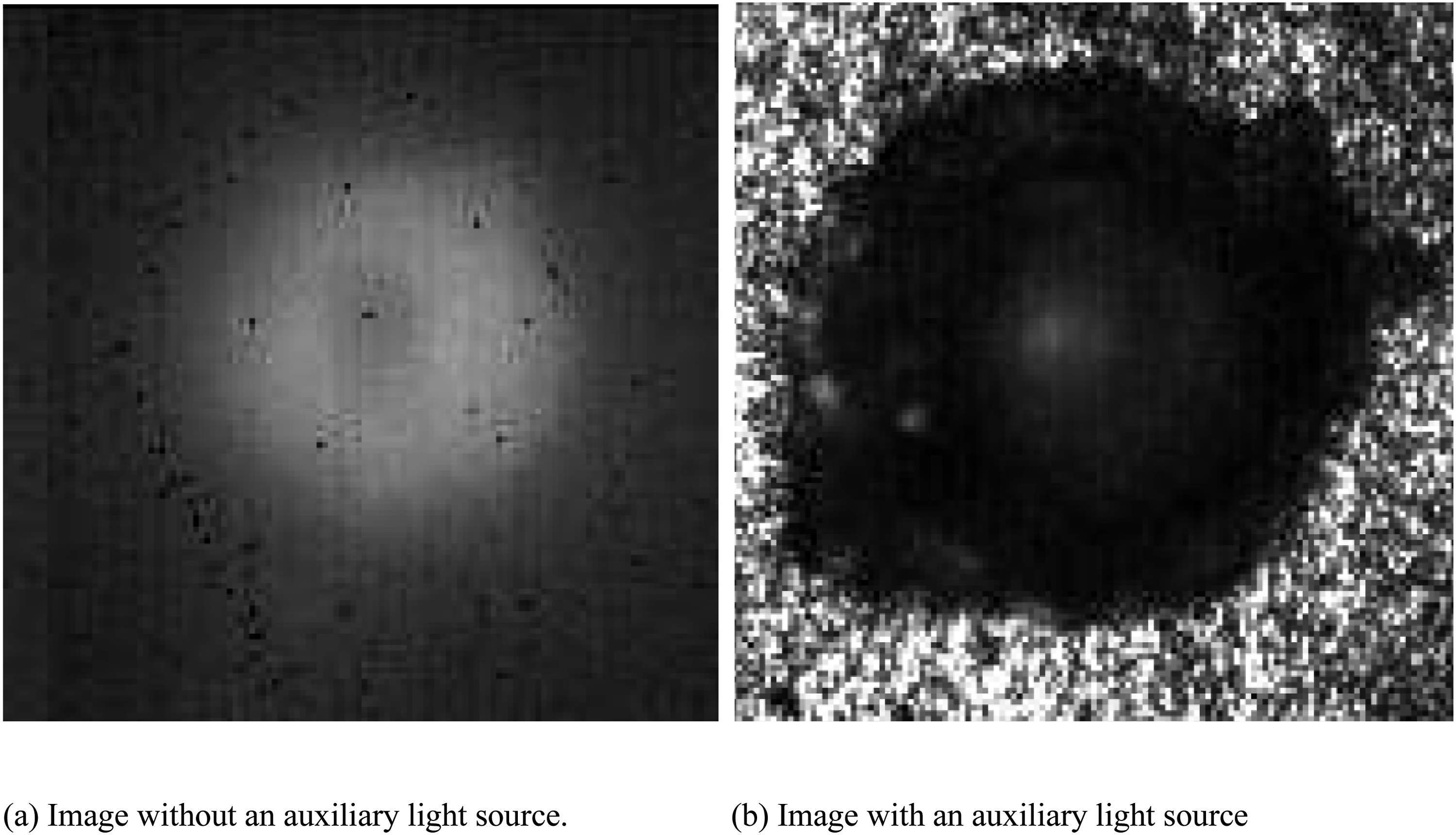

Neural network design

The RBFNN is characterized by the use of radial basis functions—most commonly Gaussian kernels—as the activation functions for its hidden-layer neurons.²⁷ RBFNNs are particularly well-suited for interpolation-driven tasks, such as modeling spatially continuous light intensity distributions in weld pools or reconstructing transient thermal fields, owing to their inherent local approximation properties.²⁸ In contrast to global approximators like multilayer perceptrons (MLPs), RBFNNs utilize radially symmetric, localized basis functions centered around predefined points in the input space.²⁹ This localized activation mechanism enables accurate interpolation between sparsely or irregularly distributed measurement points, thereby effectively capturing sharp spatial gradients and local variations that are characteristic of molten pool optical data and dynamic thermal profiles.

The spatiotemporal light intensity distribution of the molten pool is described by a function $φ = φ (s)$ , parameterized by a composite variable $s = s (r, t)$ that encompasses spatial position $r$ and time $t$ . While physics-based determination of $φ (s)$ typically involves solving complex differential equations, deriving their closed-form analytical solutions from experimental measurements is often intractable. Nonparametric statistical models are well-suited to addressing problems of this nature.³⁰ To depict the light intensity distribution, this study employs the following approximation:

φ (s) = G (φ (s^{'} \in S (s)), σ)

(1)

Here, $φ (s^{'} \in S)$ denotes the light intensity distribution at a known time instant, while $φ (s)$ represents the intensity distribution at an unknown time. The parameter $σ$ is associated with experimental conditions, and $S$ denotes the sampling domain of the variable $s$ . The field generator G is designed to compute the future spatial distribution of the field from its historical distribution.

This RBFNN constitutes a specialized three-layer feedforward architecture distinguished by its mathematically interpretable hidden-layer design.³¹ The input layer operates as a passive signal distributor, transmitting multidimensional input vectors to the hidden layer without performing nonlinear transformations.³² Each hidden neuron implements a radially symmetric basis function defined by two learnable parameters: its center vector, which positions the function in the input space, and its width parameter, which controls the radius of its local influence.³³ This parametric formulation enables the network to construct a smooth, continuous output surface through a linear combination of locally activated basis functions, rendering it particularly effective for reconstructing spatially continuous fields—such as thermal or optical distributions—from sparse or irregularly sampled measurements. This RBFNN possesses several notable characteristics:

● Static and memoryless architecture: This RBFNN employs a strictly feedforward structure without feedback or recurrent connections, resulting in a memoryless and deterministic mapping from input to output.

● Theoretical foundations in function approximation: The network is rigorously grounded in function approximation theory, providing strong mathematical guarantees for representing continuous nonlinear mappings under well-defined conditions.

● Unique global optimum under mild regularity: Under mild regularity conditions—such as linear independence of the basis functions—the network guarantees the existence of a unique global optimum for the approximation problem, simplifying training and improving solution stability.

● Linear output mapping: The transformation from the output-layer weights to the final network output is strictly linear, allowing efficient optimization via linear least-squares methods while preserving the expressive power of the hidden-layer representations.

Owing to its nonlinear approximation capability, natural suitability for spatial function learning, and efficient training, this RBFNN constitutes a powerful and appropriate computational intelligence tool for building high-fidelity predictive models of molten pool light intensity distribution, directly supporting advanced process monitoring and control in laser welding. The spatiotemporal relationship between and its sampling domain is illustrated in Figure 3. Consequently, the intensity distribution at an unknown time can be inferred from the known distribution using Eq. (1).

Figure 3.

Dependence of the variable 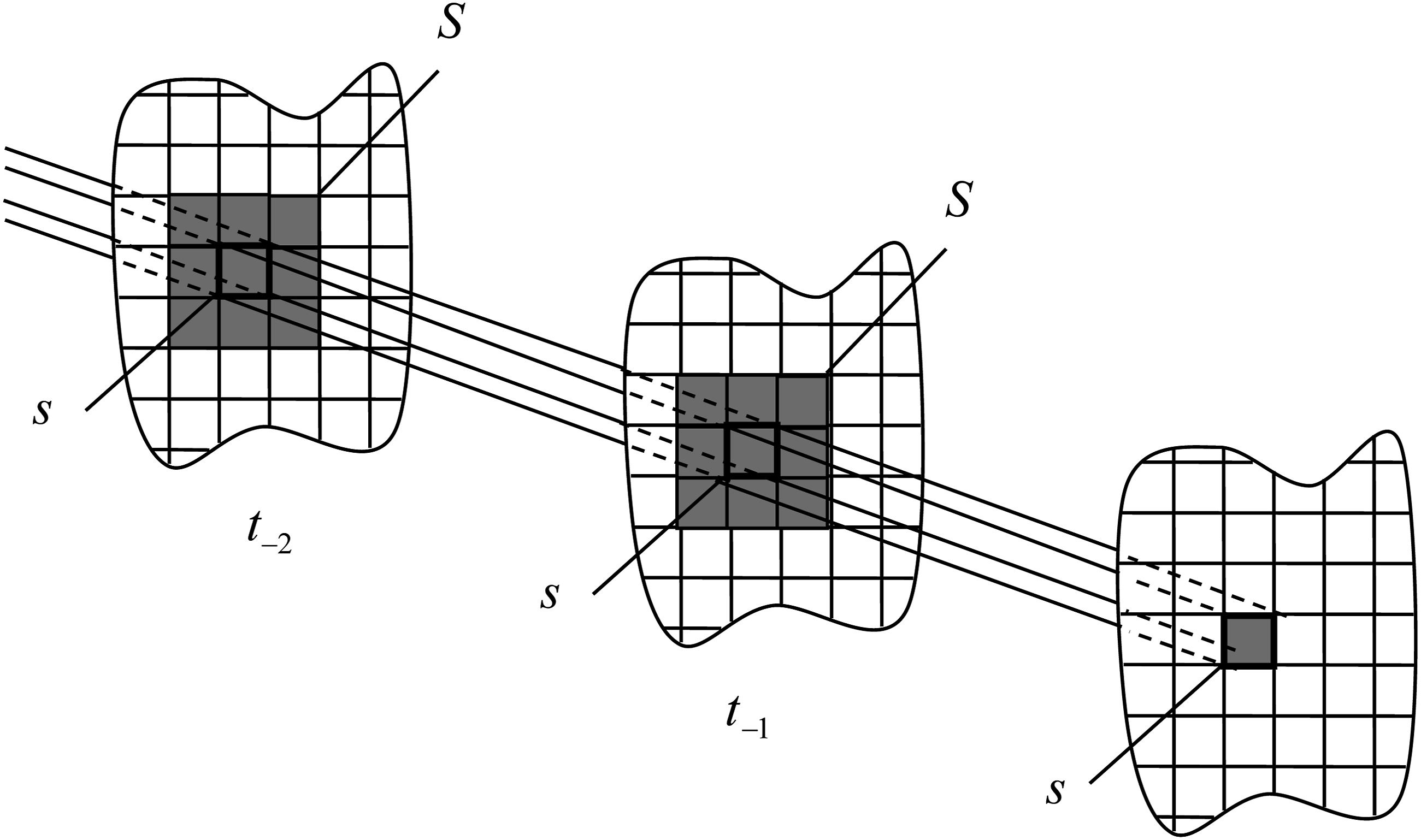$s$ on the sampling domain $S$ .

A sample vector $\vec{V} (s) = (φ_{i} (s), φ_{i} (s^{'} \in S))$ can be constructed from $φ (s)$ and $φ (s^{'} \in S)$ . For notational convenience and analytical tractability,⁹ let $x_{i} = φ_{i} (s^{'})$ , $y_{i} = φ_{i} (s)$ , then ${\vec{V}}_{i} (s) = (y_{i}, x_{i})$ . ${\vec{V}}_{i}$ is a random variable, the joint probability distribution function exists:

f_{N} (\vec{V}) = \frac{1}{N} \sum_{i = 1}^{N} ϕ (\vec{V} - {\vec{V}}_{i}, σ)

(2)

In the above expression,

N

denotes the number of sample vectors, and

ϕ

represents the set of all admissible basis functions, which here are chosen as Gaussian functions¹⁰:

ϕ (x - x_{i}, σ) = 1 / (\sqrt{2 π} σ) \exp (- {(x - x_{i})}^{2} / 2 σ)

, where

σ

is the width parameter of the function, governing its radial effective range. For optimal prediction accuracy, the mean squared prediction error (MSPE) is minimized:

E [{(y - \hat{y})}^{2} | x] = \min (\hat{y})

(3)

From Eq. (2) and (3), the conditional mean estimator can be obtained:

\hat{y} (x) = \frac{\sum_{i = 1}^{N} y_{i} ϕ (x - x_{i}, σ)}{\sum_{j = 1}^{N} ϕ (x - x_{j}, σ)} = \sum_{i = 1}^{N} y_{i} C_{i} (x)

(4)

Based on the conditional mean estimator described in Eq. (4), a RBFNN is constructed, where $(x)$ and $\hat{y} (x)$ serve as the input and output of the network, respectively. Since $\sum_{i = 1}^{N} C_{i} (x) = 1$ , the network constitutes a normalized RBFNN.

Quality assessment of prediction results

To quantitatively evaluate the predictive performance of the proposed model, the Root Mean Square Error (RMSE) is employed as the primary evaluation metric. RMSE measures the pixel-wise difference between the predicted intensity distribution $I_{p r e d}$ and the experimentally measured ground truth $I_{\exp}$ . It is defined as:

R M S E = \sqrt{\frac{1}{M \times N} \sum_{i = 1}^{M} \sum_{j = 1}^{N} {[I_{p r e d} (i, j) - I_{\exp} (i, j)]}^{2}}

(8)

where

M

and

N

are the height and width of the molten pool image in pixels, and

I (i, j)

denotes the normalized light intensity at pixel coordinate

(i, j)

. A lower RMSE value indicates higher prediction accuracy.

RMSE is adopted as the primary evaluation metric due to its direct compatibility with the specific characteristics of the prediction task. The output of the normalized RBFNN model is the normalized light intensity distribution across the molten pool, with values strictly bounded within the range [0, 1]. Under this normalization, RMSE provides an immediately interpretable measure of prediction accuracy: an RMSE value directly represents the average prediction error relative to the full intensity scale. Furthermore, because the prediction target is a two-dimensional spatial field, RMSE aggregates per-pixel discrepancies across the entire image domain, offering a comprehensive assessment of the model’s ability to reconstruct both the magnitude and spatial distribution of the light intensity. The squared term in RMSE imposes a heavier penalty on larger errors, which is particularly desirable for this application, as it ensures that significant local deviations—such as those occurring in regions with steep intensity gradients—are appropriately emphasized. Consequently, RMSE serves as a transparent, physically meaningful, and field-standard metric for quantifying the predictive performance of the proposed normalized RBFNN.

Model training and performance evaluation

This process involves three key steps.

1) Sample Vector Construction (Learning): This step involves constructing the sample vectors that form the basis for the neural network’s learning process:

(φ_{i} (s), φ_{i} (s^{'} \in S)) = (x_{i}, y_{i})

(7)

2) Prediction via Eq. (4): The target variable $\hat{y}$ is predicted by applying the computational model defined in Eq. (4).

3) Performance quantification via Eq. (4): When actual measurements are available, the predictive performance is quantified and evaluated according to the quality specified in Eq. (4).

A total of 100 experimental molten pool images were collected. The dataset was randomly partitioned into three independent subsets:

• Training set (70% of the data): Used to optimize the network parameters.

• Validation set (15% of the data): Used to monitor training progress and to tune hyperparameters (e.g., the number of RBF centers and the regularization coefficient).

• Test set (15% of the data): Used only for the final evaluation of model performance. The test set was not exposed to the model during any stage of training or validation.

To ensure that samples from all process conditions are represented in each subset, a stratified random sampling strategy was adopted. The normalized RBFNN was trained by minimizing the mean squared error (MSE) between the predicted and ground truth normalized intensities. The Levenberg-Marquardt algorithm was employed for optimizing the output weights, while the centers and widths of the radial basis functions were initialized using k-means clustering and the P-nearest neighbor heuristic, respectively, followed by fine-tuning via gradient descent.

To evaluate the model’s generalization ability beyond the training distribution, the following procedures were implemented:

1) Cross-validation: Five-fold cross-validation was performed on the training set to select optimal hyperparameters.

2) Unseen process conditions: The test set included process parameter combinations that were not present in the training set.

3) RMSE monitoring: Prediction errors on the independent test set were compared against training and validation errors to detect potential overfitting.

Results

Evaluation metric RMSE

Figure 4 illustrates the variation of RMSE as a function of the number of Gaussian radial basis functions (centers) during model optimization. As the number of centers increases, RMSE decreases rapidly initially, reaching a minimum value of 0.025 when the center count is 4. Beyond this point, further increasing the number of centers leads to a slight increase in RMSE, indicating a risk of overfitting. This result confirms that an RBFNN with 6 centers provides the optimal trade-off between predictive accuracy and model complexity.

Figure 4.

Dependence of RMSE on parameter 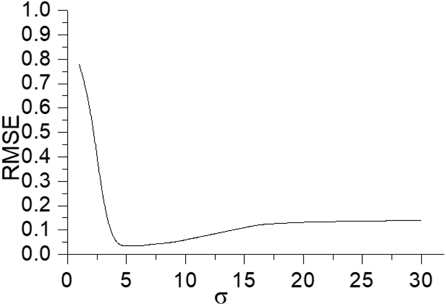$σ$ .

In Figure 4, the number of learning samples is N = 100. The sampling domain consists of fixed spatial coordinates, with only the temporal coordinate t_-1 (see Figure 3) being varied. Each reported RMSE value represents the average of 10 repeated trials under identical conditions. As can be seen from Figure 4, the RMSE value reaches its minimum when σ≈ 4. A further increase in σ leads to a slight degradation in the RMSE value. This phenomenon can be explained as follows: when σ is relatively small, the inputs that are closest to the ground truth exert the dominant influence on the prediction. Conversely, when σ is too large, the accumulated influence from inputs with greater deviations from the ground truth begins to adversely affect the overall prediction quality.

Optimization of the learning sample size N

For the model defined in Eq. (4), the computational cost of the RBFNN prediction process scales linearly with the number of learning samples N. To improve computational efficiency while maintaining prediction accuracy, the objective is to determine the minimum N that preserves the desired level of predictive performance. This trade-off was investigated empirically, yielding the characteristic performance curve shown in Figure 5.

Figure 5.

Dependence of RMSE on sample size N.

In Figure 5, the sampling domain S corresponds to that used in Figure 4, with the parameter σ fixed at its previously determined optimum of 4. All reported RMSE values represent the mean of 10 independent experimental repetitions. The results indicate a distinct trend: prediction quality, quantified by RMSE, improves markedly as the sample size N increases to approximately 400. Beyond N ≈ 600, however, further augmentation of the sample size produces only diminishing returns in predictive performance.

Optimization of the sampling domain

The sampling domain S is defined within a two-dimensional spatial and a one-dimensional temporal coordinate system. Its configuration directly governs both the complexity and the computational burden of the prediction process. Consequently, the objective is to identify the minimally sufficient sampling domain S that preserves predictive accuracy. Figure 6 illustrates the distribution of RMSE values obtained from 15 representative configurations of S, highlighting the impact of domain selection on prediction performance.

Figure 6.

Relationship between the sampling domain and prediction quality. (a) Distribution of the prediction quality (b) Schematic of the sampling domain S.

Across all experimental configurations, the parameters were held constant at σ= 4 and N = 600. Each reported RMSE value corresponds to the mean of 10 repeated trials conducted under identical processing conditions. The sampling strategy differed among conditions: configurations 1–6 employed a single temporal sampling point t_-1, while configurations 7–15 incorporated multiple time points within the defined temporal domain.

Based on the results presented in Figure 6, the following conclusions can be drawn:

● Spatial Sampling Efficiency: Under a fixed number of temporal sampling points, configurations with lower spatial sampling density consistently achieve lower RMSE values. This trend is evident from the comparative performance of conditions 1–6 versus 7–9 in Figure 6, implying that an optimal spatial sampling threshold exists beyond which additional points do not enhance—and may even reduce—prediction accuracy.

● Temporal Sampling Advantage: When spatial sampling is held constant, the inclusion of two temporal sampling points (e.g., t_-1 and t_-2) generally results in superior predictive performance, as quantified by RMSE (i.e., lower RMSE values indicate better performance). This improvement is clearly demonstrated by the significant performance gaps observed between conditions 1 and 7, and between conditions 13 and 14 in Figure 6, highlighting the importance of multi-temporal sampling for capturing process dynamics.

Modeling for the prediction of molten pool light intensity

To validate the effectiveness of the optimized parameters and sampling strategy, predicted light-intensity distributions for two representative cases are presented in Figures 7 and 8. In each figure, subfigure (a) displays the predicted distribution, whereas subfigure (b) shows the corresponding experimental measurement. Subfigure (c) presents the corresponding residual distribution map, illustrating the spatial prediction error. The spatial coordinates are denoted by r_x and r_y, and the optical intensity is represented by the variable ϕ.

Figure 7.

Predicted vs. measured light intensity distributions (Group 1). (a) predicted distribution (b)experimental measurement (c) redidual contour map of molten pool light intensity predicition.

Figure 8.

Predicted vs. measured light intensity distributions (Group 2). (a) predicted distribution (b)experimental measurement (c) redidual contour map of molten pool light intensity predicition.

To quantitatively evaluate the prediction accuracy of the proposed RBFNN model, RMSE was computed for 100 test samples covering laser powers from 750W to 1000W and focal positions from 2 mm to 8 mm (see Data Availability Statement). As summarized in Table 2, the model achieves a mean RMSE of 0.035 ± 0.006, with a minimum of 0.027 (850W/4 mm) and a maximum of 0.049 (750W/8 mm and 1000W/8 mm).

Table 2.

Statistical summary of local prediction errors across different spatial regions of the molten pool.

Spatial region	Description	Mean absolute error (MAE)	Max absolute error	RMSE
Center	Central area where laser directly irradiates, characterized by peak intensity and steep gradients	0.041	0.089	0.052
Intermediate zone	Annular region between center and boundary, where intensity decreases relatively smoothly	0.028	0.056	0.035
Boundary	Peripheral region where molten pool transitions to solid metal, marked by sharp intensity drop	0.039	0.072	0.047
Full molten pool	Entire ROI (all pixels within the molten pool area)	0.032	0.089	0.037

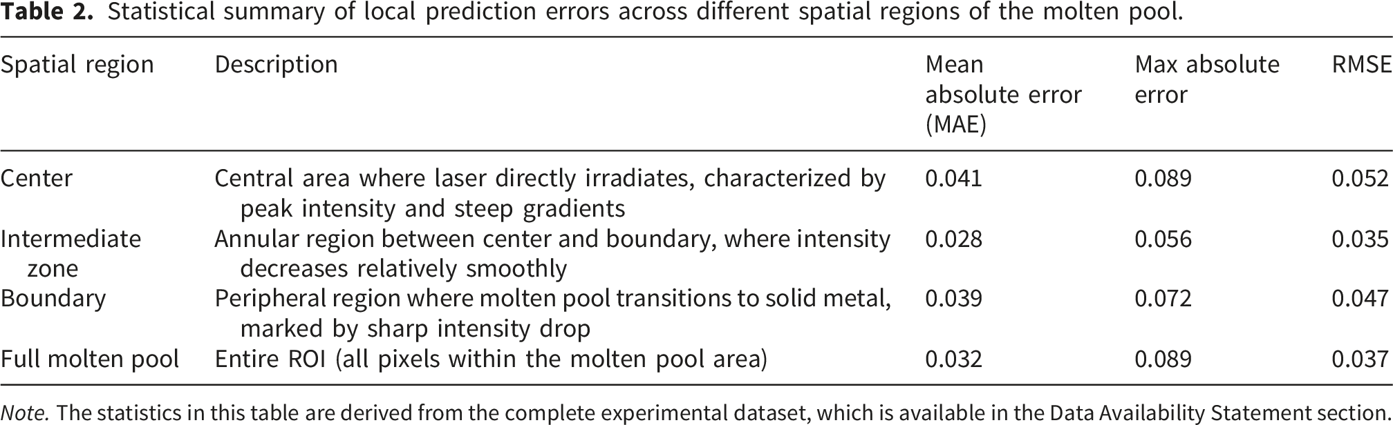
Note. The statistics in this table are derived from the complete experimental dataset, which is available in the Data Availability Statement section.

A spatial breakdown of errors (Table 2) shows that the center region exhibits the highest errors (MAE=0.041, RMSE=0.052), the boundary region shows elevated errors (MAE=0.039, RMSE=0.047), and the intermediate zone yields the lowest errors (MAE=0.028, RMSE=0.035). These results confirm that prediction accuracy varies systematically with spatial region and that prediction difficulty is intrinsically linked to the local physical characteristics of the molten pool.

Discussion

This study establishes a data-driven spatiotemporal model for predicting the molten pool luminous intensity distribution in laser welding, addressing the long-standing challenge of modeling complex optical phenomena in dynamic thermal processes. The results demonstrate that the integration of a structured neural architecture with a systematic optimization framework can effectively capture and reconstruct welding signatures with high fidelity.

The primary methodological contribution of this work is threefold. First, we introduce a physically-informed neural network design that embeds Gaussian radial basis functions into a nonparametric architecture. Unlike classification-oriented approaches, our method directly predicts the continuous two-dimensional light intensity field, offering richer information for process monitoring without requiring manual feature engineering. Second, we adopt the Root Mean Square Error (RMSE) as the primary evaluation metric, which provides an interpretable and physically meaningful measure of prediction accuracy. The squared term in RMSE naturally penalizes larger errors, aligning the model optimization with the engineering priority of avoiding significant prediction deviations. As a purely data-driven model, our approach also avoids the complexity and domain-knowledge requirements of hybrid physical-data-driven models while achieving high accuracy (mean RMSE = 0.035 across 100 test conditions). Third, we implement a closed-loop hyperparameter optimization procedure that automates the tuning process based on this metric, significantly reducing expert dependency and improving reproducibility in model deployment. By enabling accurate and efficient prediction of the molten pool’s fundamental optical signature, this study provides a new computational tool for real-time laser welding monitoring and quality assessment, contributing to the advancement of intelligent manufacturing.

Prediction errors are not uniformly distributed across the molten pool but concentrate along steep intensity gradient zones corresponding to the solid-liquid interface and keyhole periphery, where strongly nonlinear dynamics—Marangoni convection, recoil pressure, and rapid phase changes—govern the process; the RBFNN maintains low RMSE in these challenging areas, suggesting that its localized Gaussian kernels effectively capture the dominant spatial modes of temperature-induced radiation. A key strength of the proposed approach is its nonparametric nature, which allows it to learn mappings directly from experimental data and implicitly account for complex mechanisms such as plume attenuation and keyhole reflections. However, several limitations must be acknowledged: the model is trained on a specific material and limited parameter range, it does not provide prediction uncertainty estimates critical for safety-critical applications, and it excludes temporal dynamics of the melt pool. Practically, real-time full-field intensity prediction enables model-based closed-loop control with spatially resolved parameter adjustments; academically, this work demonstrates that a nonparametric neural network can serve as a surrogate digital twin for welding processes. Future work should extend to multi-material scenarios, incorporate temporal dynamics, and explore transfer learning to reduce experimental data requirements. These methodological advancements collectively offer a transferable framework for spatiotemporal modeling in optical monitoring of thermal processes; the approach is not merely an application of existing neural networks, but a structured methodology that balances data-driven flexibility with physical plausibility—a critical step toward trustworthy AI in manufacturing. The RBFNN offers a fast, low-complexity alternative to both physics-based models and heavier deep learning networks, providing a balanced perspective on data-driven molten pool modeling.

Conclusion

This study establishes a novel predictive framework for the spatiotemporal light intensity distribution in laser welding molten pools, with its core innovation lying in the systematic integration of a normalized RBFNN with nonparametric statistical regularization. The proposed RBFNN-based model explicitly encodes the locally dominant optical-thermal interactions through spatially adaptive Gaussian kernels, enabling faithful reconstruction of intensity fields without relying on empirical or globally parameterized physical assumptions. Its linear-in-parameters output structure and locally supported basis functions ensure training stability, computational efficiency, and interpretability—advantages seldom achieved in conventional deep learning architectures. Furthermore, the model successfully captures underlying process dynamics, as evidenced by the consistent correlation between its spatially resolved activation patterns and experimentally observed thermal-optical phenomena. By bridging the rigorous function approximation capability of RBFNNs with the adaptability of nonparametric learning, this work provides a physically consistent, data-efficient, and real-time capable computational tool for welding monitoring, with direct relevance to adaptive control and quality assurance in intelligent manufacturing systems.

Footnotes

Acknowledgments

The authors would like to thank the National Natural Science Foundation of China and the Natural Science Foundation of Tianjin for their valuable support in this work.

ORCID iD

Jian Zhang

Author contributions

Jian Zhang conceived and designed the study; Rui Yang collected the data; Xiaoxi Dong performed the data analysis; Huijuan Yin contributed to data interpretation and visualization; Rui Yang and Xiaoxi Dong drafted the initial manuscript; Huijuan Yin revised the manuscript critically for important intellectual content; and Jian Zhang supervised the overall research process and managed the project. All authors read and approved the final version of the manuscript.

Funding

The authors disclosed receipt of the following financial support for the research, authorship, and/or publication of this article: This study was supported by the National Natural Science Foundation of China (62175261) and the Natural Science Foundation of Tianjin (24JCZDJC00240).

Declaration of conflicting interests

The authors declared no potential conflicts of interest with respect to the research, authorship, and/or publication of this article.

Data Availability Statement

The quantitative prediction error data (RMSE values) generated and analyzed during this study are available in the Figshare repository under the following link: .³⁴

References

Shen

, et al. Simulation Study on Laser Welding Parameters of Al6063-T6 Aluminum Tubes. In: Proceedings of the 8th International Conference on Electrical. Mechanical and Computer Engineering, (ICEMCE), Xi’an, China, 25-27 October 2024, pp. 343–347.

BasiReddy Peddapudi

Sravanthi

Uppalapati

, et al. Distortion measurement of Laser beam welding for Similar and Dissimilar joints using a Coordinate Measuring Machine. In: Proceedings of the 1st International Conference on Innovative Engineering Sciences and Technological Research, (ICIESTR). Oman, Muscat, 14-15 May 2024, pp. 1–5.

Bui Thi

Pham

Duong

, et al. Research, Design, Fabrication of Automatic Battery Cell Welding Machine to Support Maintenance and Replace Damaged Battery Generation for Electric Vehicles. In: Proceedings of the 10th International Conference on Applying New Technology in Green Buildings, (ATiGB 2025), Danang, Vietnam, 25-26 July 2025, pp. 751–757.

Xiao

, et al. An Autonomous Laser Stripe Feature Point Extraction Algorithm Based on Siamese Network for Robotic Welding Seam Tracking. IEEE Transactions on Industrial Electronics 2024; 71(1): 1037–1048. https://doi.org/10.1109/tie.2023.3243265

Huang

Luo

, et al. Numerical simulation of laser transmission welding of PEEK and CF-PEEK composite pipe fittings. In: Proceedings of the 8th International Conference on Electrical, Mechanical and Computer Engineering, (ICEMCE), Xi’an, China, 25-27 October 2024, pp. 1263–1268.

Tao

Liu

, et al. Electron Beam Welding of the HTS Current Lead for the ITER Feeder. IEEE Transactions on Plasma Science 2024; 52(11): 5451–5456. https://doi.org/10.1109/tps.2024.3495636

Huang

Han

Liu

, et al. Prediction of Laser-TIG Weld Profile Based on Neural Network and Intelligent Detection. In: Proceedings of the 4th International Conference on Artificial Intelligence and Advanced Manufacturing, (AIAM), Hamburg, Germany, 7-9 October 2022, pp. 578–582.

Mazzoleni

Demir

Caprio

, et al. Real-Time Observation of Melt Pool in Selective Laser Melting: Spatial, Temporal, and Wavelength Resolution Criteria. Transactions on Instrumentation and Measurement 2020; 69(4): 1179–1190. https://doi.org/10.1109/tim.2019.2912236

Sikström

Nilsen

, et al. Deep Learning for Joint Gap Width Classification and Tack Weld Detection in Laser Beam Welding. In: Proceedings of New Trends in Signal Processing, (NTSP), Demanovska Dolina, Slovakia, 16-18 October 2024, pp. 1–6.

10.

Yan

Mei

. Simulation of the effects of Activators on the Laser Welding of Stainless Steel Plate. In: Proceedings of International Conference on Manufacturing, Industrial Automation and Electronics, (ICMIAE), Rimini, Italy, 26-28 August 2022, pp. 407–412.

11.

Bopalkar

Patwardhan

Okello

, et al. Impact of Laser Welding on Assembly of Printed Circuit Boards in Medical Devices. In: Proceedings of IEEE CPMT Symposium Japan, (ICSJ), Kyoto, Japan, 13-15 November 2024, pp. 112–115.

12.

Chen

. Identification of Ionization Region Profile and Potential Distribution in Welding Arc Plasma by Direct Probe Detection. IEEE Transactions on Plasma Science 2023; 1(7): 2004–2009. https://doi.org/10.1109/tps.2023.3282986

13.

Fan

Gao

, et al. Prediction of Weld Widths for Laser-MIG Hybrid Welding Using Informer Model. Transactions on Industrial Electronics 2024; 71(6): 6221–6230. https://doi.org/10.1109/tie.2023.3294634

14.

Fan

Hou

, et al. Vision-Based Autonomous Robotic Arc Welding: State-of-the-Art Review and Perspectives. Transactions on Automation Science and Engineering 2025; 22: 21651–21673. https://doi.org/10.1109/tase.2025.3614992

15.

Omlor

Reith

Breitbarth

, et al. Inline Process Monitoring of Hairpin Welding Using Optical and Acoustic Quality Metrics. In: Proceedings of the 12th International Electric Drives Production Conference, (EDPC), Regensburg, Germany, 29-30 November 2022, pp. 1–8.

16.

Haiyun

Chunchen

, et al. Effect of gas hole in laser deep penetration welding of superalloy on welding strength. In: Proceedings of the 15th International Conference on Reliability, Maintenance and Safety, (ICRMS), Guilin, China, July 31-August 3 2024, pp. 487–492.

17.

Wang

Feng

Jiang

, et al. Multi-physics characterization of molten pool via an online in situ monitoring system in metal additive manufacturing. Journal of Manufacturing Processes 2026; 157: 352–370. https://doi.org/10.1016/j.jmapro.2025.11.059

18.

Zhang

Huang

, et al. Detection of variable-groove weld penetration based on cooperative awareness of melt pool vision and temperature field. Optics & Laser Technology 2025; 184: 112432. https://doi.org/10.1016/j.optlastec.2025.112432

19.

Zhang

, et al. Progress and perspectives of in-situ optical monitoring in laser beam welding: Sensing, characterization and modeling. Journal of Manufacturing Processes 2022; 75: 767–791. https://doi.org/10.1016/j.jmapro.2022.01.044

20.

Long-Zhang

Wen-Liang

Xiao-Yan

, et al. Nonlinear effect of laser frequency modulation on molten pool width in deep penetration laser welding. Optics & Laser Technology 2016; 194: 114445. https://doi.org/10.1016/j.optlastec.2025.114445

21.

Vigneswaran

Vignesh

Qureshi

, et al. A Novel AMB Laser Welding of Copper Eyelets onto Aluminum Busbars. In: Proceedings of the 3rd International Conference on Power, Control and Computing Technologies, (ICPC2T). India, Raipur, 18-20 January 2024, pp. 114–117.

22.

Kim

Kang

Kim

, et al. Al-Driven Interfacial Gap Prediction in Overlapped Al/Cu Laser Weld Joint for Battery Applications. IEEE Access 2025; 13: 181302–181312. https://doi.org/10.1109/access.2025.3621683

23.

Vater

Kirschning

Knoll

. Closing the loop: Real-time Error Detection and Correction in automotive production using Edge-/Cloud-Architecture and a CNN. In: Proceedings of International Conference on Omni-layer Intelligent Systems. Barcelona, Spain Coins, August 31-September 2 2020, pp. 1–7.

24.

Kabalan

Asad

Motawej

. Effect of Plasma Mode Frequency on Gaussian Laser Beam in Hot Plasma. IEEE Transactions on Plasma Science 2024; 52(6): 2013–2020. https://doi.org/10.1109/tps.2024.3426555

25.

Bernatskyi

Sokolovskyi

Nabok

, et al. Development of a Model Device of a Control System Device for Control of the Power Source for Hybrid Laser-Arc Welding of Aluminium Alloys. In: Proceedings of the 4th International Conference on Modern Electrical and Energy System, (MEES), Kremenchuk, Ukraine, 20-23 October 2022, pp. 1–6.

26.

Olsson

Eriksson

Powell

, et al. Challenges to the interpretation of the electromagnetic feedback from laser welding. Optics & Lasers in Engineering 2011; 49(2): 188–194. https://doi.org/10.1016/j.optlaseng.2010.08.018

27.

Broomhead

. Lowe and David. Multivariable functional interpolation and adaptive networks. Complex Systems 1988; 2(3): 321–355.

28.

Sui

Han

Liu

, et al. Optimal Chaos Sequence Prediction Based on Optimized Radial Basis Function Neural Network. In: Proceedings of the 2nd International Conference on Signal Processing and Intelligent Computing, (SPIC), Guangzhou, China, 20-22 September 2024, pp. 361–364.

29.

Gangolu

Chauhan

Dwivedi

, et al. Fault Classification in Transmission Lines Using Radial Basis Function Neural Networks. In: Proceedings of the 11th Power India International Conference, (PIICON), India, Jaipur, 10-12 December 2024, pp. 1–6.

30.

Dat

Shue

Guan

. Electrocorticographic signal classification based on time-frequency decomposition and nonparametric statistical modeling. In: Proceedings of International Conference of the IEEE Engineering in Medicine and Biology Society. New York, NY, USA, August 30-September 3, 2006, pp. 2292–2295.

31.

Hušek

. On Monotonic Radial Basis Function Networks. IEEE Transactions on Cybernetics 2024; 54(2): 717–727. https://doi.org/10.1109/tcyb.2022.3185827

32.

Karpagavalli

Kaliappan

Amuthachenthiru

. Radial Basis Function Neural Network for Intrusion Detection and Feed Forward Artificial Neural Network for Attack Mitigation in IoT. In: Proceedings of the 2nd International Conference on Augmented Intelligence and Sustainable Systems, (ICAISS), Trichy, India, 23-25 August 2023, pp. 1239–1245.

33.

Behera

Mohanty

Kumar Dash

, et al. Radial Basis Neural Networks for Class Discovery. In: Proceedings of OITS International Conference on Information Technology, (OCIT), India, Bhubaneswar, 14-16 December 2022, pp. 330–334.

34.

Zhang

. Quantitative prediction errors of the radial basis function neural networkmodel across different welding parameters. figshare. Dataset 2026. https://doi.org/10.6084/m9.figshare.32095810.v1.